Cooling by heating a nanodroplet - proof of concept

Abstract

Recently [3] predicted the existence of an intriguing new phenomenon. It was shown that if temperature is suddenly raised at the surface of a sphere the temperature in the interior initially decreases. The authors of [3] gave a thorough analysis explaining the physics leading to this remarkable effect. They linked the existence of the phenomenon to the subtle thermomechanical coupling between displacement and temperature in a sphere that is able to expand freely and showed that the effect is expected to be largest close to the glasstransition temperature of the perturbed material. The prediction was based on the assumption of quasi-elasticity where the sample is much smaller than the wavelength of acoustic waves at frequencies of relevance. Being in the inertia free limit they could ignore the acceleration term in the thermoviscoelastic equations of motion. Here we give the first empirical proof of existence of the effect by performing molecular dynamics simulations of a supercooled Kob-Andersen binary mixture of Lennard-Jones particles forming a droplet consisting of 500.000 particles. We show that the phenomenon is real even when inertia cannot be disregarded.

1 Introduction

The thermoviscoelastic nature of viscous liquids gives rise to a rich phenomenology [1] and pose fundamental challenges in science [2]. Recently [4, 5] discuss the breaking of hydrostatic conditions that occurs when the release of stresses that arise from thermal waves take place on the timescale of experiment (the stress tensor is temporarily nonisotropic). Papini and coauthors [3] analyze this breaking of hydrostatic conditions and its consequences pertaining to two cases of heating a spherical sample through the mechanically free surface. E.g. as a finite amount of heat is added at the surface, the interior of the sphere, even close to the surface, instantaneously cools to a common temperature independent of radius; the expansion of the surface is immediately felt in the interior and as no heat has been transfered it cools adiabatically. They explain the phenomenon and give the conditions for its existence in terms of a subtle thermomechanical coupling, that peaks in the glass transition region of a material.

It all boils down to the nature of longitudinal expansion, which is present when you heat a sphere homogenously at its surface. The thermomechanical coupling can be quantified by the relative difference between the longitudinal specific heat, $c_{l}$ and the isobaric specific heat, $c_{p}$, that are defined in Eq’s (1) and (2):

$$c_{l}=\frac{M_{S}}{M_{T}}c_{V}$$ (1)

$$c_{p}=\frac{K_{S}}{K_{T}}c_{V},$$ (2)

where $K_{S}$ and $K_{T}$ are the adiabatic and isothermal bulkmoduli respectively and $c_{V}$ is the isochoric specific heat. The longitudinal moduli are given by $M_{S}=K_{S}+4/3\,G$ and $M_{T}=K_{T}+4/3\,G$ with $G$ being the shear modulus. The authors of [3] point out that the difference between $c_{l}$ and $c_{p}$ only occurs when two conditions are met simultaneously. First, shearmodulus must be nonvanishing compared to bulkmodulus and second, the adiabatic and isothermal bulkmoduli must differ significantly. This situation will be most probable near the glass transition where the constitutive quantities become frequency dependent. Combining Eq’s. (1) and (2) they show that the effect they term “Cooling by heating” only occurs when the resulting thermo-mechanical coupling constant $a$ defined as

$$a\equiv\frac{c_{p}-c_{l}}{c_{p}}=\frac{4}{3}\cdot\frac{G}{M_{T}}\cdot\frac{c_{p}-c_{V}}{c_{p}},$$ (3)

differs from zero.

The analyzis given in [3] is based on the assumption of quasi-elasticity where they could ignore the acceleration term in the thermoviscoelastic equations of motion for temperature $\delta T(r,s)$ and displacement $\textbf{u}(r,s)=u(r,s)\textbf{r}$ in the frequency domain [5]:

$$\boldsymbol{\nabla}\left(M_{T}\boldsymbol{\nabla}\cdot\textbf{u}-\alpha_{p}K_{T}\delta T\right)=\rho s^{2}\textbf{u}$$ (4)

$$c_{V}s\delta T+T_{0}\alpha_{p}K_{T}\boldsymbol{\nabla}\cdot\textbf{u}=\lambda\boldsymbol{\nabla}^{2}\delta T$$ (5)

Here $\alpha_{p}\equiv\frac{1}{V}\left(\frac{\partial V}{\partial T}\right)_{p}$ is the isobaric expansion coefficient, $\lambda$ the heat conductivity as defined by Fourier’s law, $s=i\omega$ the Laplace frequency with the cyclic frequency $\omega$ and $\rho$ the average mass density.

Introducing the potential function $\phi$ by $\textbf{u}=\boldsymbol{\nabla}\phi$ Eq. (4) becomes

$$\boldsymbol{\nabla}\left(M_{T}\boldsymbol{\nabla}^{2}\phi-\rho s^{2}\phi-\alpha_{p}K_{T}\delta T\right)=0.$$ (6)

Adjusting $\phi$ with an appropriate (r-independent) additive constant, the integration constant that comes out integrating Eq. (6) is set to zero. Introducing the dimensionless quantities $\alpha=T_{0}\alpha_{p}$, $c=T_{0}c_{l}/K_{T}$, $g=4G/3K_{T}$, $1/\gamma_{l}=M_{T}/M_{S}=c_{V}/c_{l}=1-\alpha^{2}/c(g+1)$ as well as the acoustic (adiabatic) and thermal wave vectors defined by $q^{2}=\rho/M_{S}s^{2}$ and $k^{2}=c_{l}s/\lambda$ respectively, Eq.’s (6) becomes, on dimensionless form:

$$\left(\boldsymbol{\nabla}^{2}-\gamma_{l}\left(\frac{q}{k}\right)^{2}\right)\phi=\frac{\alpha}{1+g}\delta T$$ (7)

As long as $q^{2}/k^{2}\ll 1$ we can safly assume non-inertial conditions. Introducing characteristic numbers for the speed of sound $c_{sound}=M_{S}/\rho\approx 10^{3}m/s$ and diffusivity $D=c_{l}/\lambda\approx 10^{-7}m^{2}/sec$ we have $\left(\frac{q}{k}\right)^{2}=\frac{D}{c_{sound}^{-2}}s=2\pi 10^{-13}\sec f$, $f$ being the frequency. When the system studied becomes extremely small, like in a nano-sized droplet, the relevant timescales (picoseconds) are exactly those where the corresponding frequencies give a $\left(\frac{q}{k}\right)^{2}\approx 1$. These frequencies, which give wavelengths, $\lambda=c_{sound}/f$, comparable to the size of the sample (nanometers) are also those that make the assumption of adiabatic propagation of acoustic waves flawed. Therefore the situation becomes much more complicated when dealing with very small samples than in the quasi-elastic case studied in [3].

To see if the phenomenon predicted in [3] is also present in nano-sized systems we performed molecular dynamics simulations of a small droplet (described below) thus giving a proof of concept regarding the existence of Cooling by heating.

2 Simulations of a nano-sized droplet

2.0.1 Preparing the simulations

The cooling by heating in a droplet is expected to be biggest at the glass transition in a supercooled fluid. Almost all Molecular Dynamics (MD) simulations [6] of supercooled systems are performed for the Kob-Andersen binary mixture of Lennard-Jones particles (KABLJ) [7]. This system consist of 80% A-particles and 20% smaller B-particles in a strong exothermic mixture, which makes it very resistant against crystallization [8]. The glas transition temperature, $T_{g}$ is estimated to be $T_{g}$=0.438 [7] for an uniform system of $N=N_{\textrm{A}}+N_{\textrm{B}}$=1000 Lennard-Jones (LJ) particles at a density, $\rho=1.2$. A droplet of only one thousand particles is, however, much too small to establish the effect and to measure it accurately, and for this reason we have created a droplet of $N$=500 000 particles. The reason for choosing such a big number is to make sure that there is time enough to measure an effects of thermomechanical coupling before everything is washed out by the diffusion of heat.

A droplet of $N$=500 000 KABLJ particles was created in the following way: A KABLJ system of $N$=1000 particles was calibrated at a density of $\rho=1.2$ and temperature $T$=0.40. A number of copies of the system were then fused into a huge system, from which a spherical droplet consisting of 500.000 particles was cut out. The droplet was then placed in a container with the box-side length 10 times bigger than the radius of the droplet [9]. Droplets were then equilibrated at 3 temperatures: $T$=0.38,0.40,0.42, all below the glas-temperature. In figure 1 we show the density profile of a droplet at the temperature $T=0.40$ with the density of the bulk $\rho=1.08$. We took the relaxation time, $\tau_{\alpha}$ of the systems to be given by the time when the AA incoherent intermediate scattering function in a KABLJ is equal to $1/e$ (at wave vector $q=7.25(\rho/1.2)^{1/3}$ [10]). Then we run simulations at the four state points, dumping configurations separated by $2\tau_{\alpha}$, creating an ensemble consisting of 300 droplets with uncorrelated start configurations at each state point.

2.0.2 Production runs

In the production runs we thermostatted the particles in the surface shell between concentric spheres at the surface of the droplet, keeping track of all the particles during the whole run. The particles in the shell were defined as those that are situated in an interval of radii from the center shown by vertical lines in figure 1. These particles were thermostated by a Nose-Hoover thermostat (NHT) [6]. The NHT thermostat consists of a "friction therm" in the classical equations of motion and the thermostat has a relaxation parameter $\tau_{T}$ which controls the heat flow into and out of the system. A big value of $\tau_{T}$ results in big and slow oscillations of the temperature $T$ around the target temperature whereas a small value of $\tau_{T}$ results in small and quick oscillations [11]. The NHT thermostated particles are not accelerated (heated) or damped (cooled) by particle collisions, but by the dynamic friction parameter in the equations of motion, by which one in general avoids thermal waves in the system if all particles are coupled to the thermostate. In the present simulations we want, however, to create a thermal wave by heating only the particles at the surface.

The thermal wave was started by increasing the thermostate temperature with $\delta T=0.02$, for particles in the surface shell. This was done in the following way. First we use a big value of $\tau_{T}$ for a short time by which the temperature change were “Heaviside-like”. At the time where the temperature reached the desired value, we switched to a smaller value of $\tau_{T}$ which immediately stabilized the temperature at the new target temperature ($T+\delta T$) in the surface shell. The NHT thermostating with the small value of $\tau_{T}$ were then continued for a short time in order to pump some heat into the surface shell. Then the thermostat were switched of, giving a constant energy in the droplet for the rest of the simulation and at the same time starting a heat wave into the droplet. The temperature evolution in the surface shell is shown in figure 2 for the step done from $T=0.40$ to $T=0.44$.

In order to calculate the local quantities, like density and temperature we divided the system into concentric shells, with some given thickness. In all the figures shown in this work we chose to divide the droplets into 10 shells. This number is based on a compromise to secure good enough statistics, especially in the innermost shells, but still get a good enough resolution in order to study the evolution of the temperature in the shells.

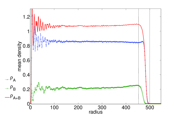
Figure 1: Density profiles, $\rho(r)$, as a function of the distance $r$ from the center in the droplet before the thermal wave was created. The KABLJ droplet consists of solvent A-particles and solule B-particles. The droplet were heated up in the surface shell at $r\approx 500\sigma_{\textrm{AA}}$, marked by the vertical lines

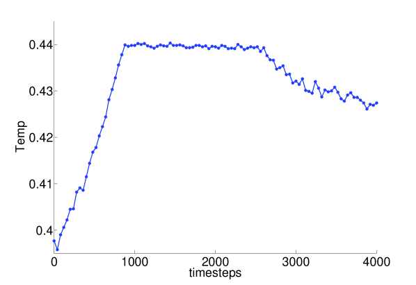
Figure 2: Temperature evolution in the thermostated surface shell at the start of the thermal wave into the droplet. After a short heating of $\approx$ 1000 timesteps with a big value of $\tau_{T}$, the shell was calibrated 2000 timesteps wit $\tau_{T}\approx\tau_{c}$. from where the surface thermostate was swiched off.

3 Results from simulations of a nanosized droplet - proof of existence

The evolution of temperature and displacement fields were analyzed in [3]. The analyse included the deduced evolution of stresses and pressure after a spherical system has been perturbed thermally at its surface. Only addition of heat, or jumps up in temperature at the surface of the sphere were, however, considered. They do not consider what effect a removal of heat, or jump down in temperature will affect. In the thermoelastic case (solid) where one can ignore memory effects and the influence of temperaure on relaxation properties of the system, one would expect the phenomenon to be symmetric with respect to the direction of heat transfer. In the case of a system whose relaxation properties change with temperature, like in a super cooled liquid, one can, however, not apriori expect a symmetric behavior because the relaxation time varies exponentially with thetemperature.

In figure 3 we show the temperature of a section of the droplet close to the surface. Here we first see the wave induced by heating or cooling at the surface followed first by the reverse characteristic cooling/heating phenomenon which again is followed by the diffusion of heat. But the phenomenon is symmetric despite the exponentially varying relaxation times in the supercooled rigime.

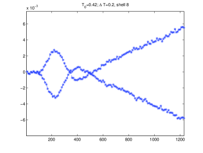
Figure 3: Temperature evolution in an inner shell (No. 8) in the droplet after the surface shell has beeen heated/cooled. The effect is symmetric with respect of the sign of the temperature step at the surface

Figure 4 shows the temperature as a function of time for a number of concentric shells in the droplet. Whe the temperature at the surface is increased it starts an acoustic wave which travels in towards the center of the sphere and results in an increase in temperature due to the thermomechanical coupling. This is followed by a temperature drop - cooling by heating, thus providing a proof of the concept introduced in [3]. We have left out the innermost shells, i.e. shells 1 and 2. The reason for this is twofold. First of all, since the number of particles in the shells - they all have the same thickness, decreases as one gets closer to the center of the droplet, the noise increases as there are fewer particles to average over. The second reason is that in the innermost parts of the droplet, the acoustic and thermal waves mix, giving a more messy picture.

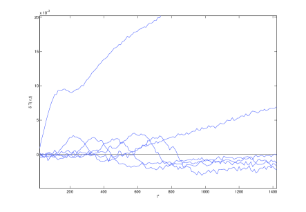
Figure 4: The temperature change as a function of time for a number of radii. The uppermost curve represents the evolution in temperature close to the surface. The curve below refers to a a radius a bit closer to the center of the droplet, and so on. For all radii one first sees the elastic wave that is induced by the step in temperature on the surface of the droplet, followed by the an increasing temperature due to the diffusion of heat. However, for the innermost parts of the droplet the elastic wave is followed by the phenomenon of Cooling by heating. The size of the effect increases the closer to the center you look.

4 Discussion

References

References

- [1] Harrison G The Dynamic Properties of Supercooled Liquids. Academic Press, 1976
- [2] Dyre J C 2006 Rev. Mod. Phys. 78 No. 3, July-September
- [3] Papini J, Christensen T, Olsen N B and Dyre J C 2011 Unknown Journal Volume X page Y
- [4] Christensen T, Olsen N B and Dyre J C 2007 Phys. Rev. E 75 041502
- [5] Christensen T and Dyre J C 2008 Phys. Rev. E 78 021501
- [6] For MD details see e.g. Toxvaerd, S. Algorithms for canonical molecular dynamics simulations. Mol. Phys. 72, 159 (1991). Unit lenght, energy and time is , and , where and is the length and the energy parameters in the LJ potential .
- [7] W. Kob and H. C. Andersen, Phys. Rev. E 51, 4626 (1993); ibid. 52, 4134 (1995).
- [8] S. Toxvaerd, U. R. Peder sen, T. Scareøder, and J. C. Dyre, J. Chem. Phys. 130, 224501 (2009).
- [9] S. Toxvaerd,i J. Chem. Phys. 117, 10303 (2002).
- [10] U. R. Pedersen, T. B Schrøder , and J. C. Dyre, Phys. Rev. Lett. 105, 157801 (2010).
- [11] A natural time unit for a MD thermostate is the mean collision time of the thermostated particles. A small value of the thermostates relaxation time, , corresponds to .