Two-scale convergence for locally-periodic microstructures and homogenization of plywood structures.

Abstract.

The introduced notion of locally-periodic two-scale convergence allows to average a wider range of microstructures, compared to the periodic one. The compactness theorem for the locally-periodic two-scale convergence and the characterisation of the limit for a sequence bounded in $H^{1}(\Omega)$ are proven. The underlying analysis comprises the approximation of functions, which periodicity with respect to the fast variable depends on the slow variable, by locally-periodic functions, periodic in subdomains smaller than the considered domain, but larger than the size of microscopic structures. The developed theory is applied to derive macroscopic equations for a linear elasticity problem defined in domains with plywood structures.

1. Introduction

Many natural and man made composite materials comprise non-periodic microscopic structures, for example fibrous microstructure with varied orientation of fibres in heart muscles, [28], in exoskeletons, [15], in polymer membranes and industrial filters, [31], or space-dependent perforations in concrete, [30]. An interesting and important special case of non-periodic microstructures is the so called locally-periodic microstructures, where spatial changes of the microstructure are observed on a scale smaller than the size of the considered domain but larger than the characteristic size of the microstructure. The distribution of microstructures in locally-periodic materials is known a priori, in contrast to the stochastic description of the medium considered in stochastic homogenization, [8].

There are few mathematical results on homogenization in locally-periodic and fibrous media. The homogenization of a heat-conductivity problem defined in locally-periodic and non-periodic domains consisting of spherical balls was studied in [11] using the Murat-Tartar $H-$convergence method, defined in [24]. The locally-periodic and non-periodic distribution of balls is given by a $C^{2}-$diffeomorphism $\theta$, transforming the centres of the balls. For the derivation of macroscopic equations for the problem posed in the non-periodic domain, where the changes of the microstructure are given on the scale of the considered microstructure, a locally-periodic approximation was considered. Estimates for the numerical approximation of this problem were derived in [32]. The notion of $\theta-2$ convergence, motivated by the homogenization in a domain with a microstructure of non-periodically distributed spherical balls, was introduced in [1]. The Young measure was used in [20] to extend the concept of periodic two-scale convergence, presented in [2], and to define the so-called scale convergence. The definition of scale convergence was mainly motivated by the derivation of the $\Gamma$-limit for a sequence of nonlinear energy functionals involving non-periodic oscillations. It has been shown that the two-scale and multi-scale convergences are particular cases of the scale convergence. In [20], as an example of non-periodic oscillations, the domain with perforations given by the transformation of centre of balls was considered. Macroscopic models for non-periodic fibrous materials were presented in [10] and derived in [9]. The non-periodic fibrous material is characterised by gradually rotated planes of parallel aligned fibres. By applying the $H-$convergence method for a locally periodic approximation of the non-periodic microstructure the effective homogenized matrix was derived. The asymptotic expansion method was used in [6] to derive macroscopic equations for a filtration problem through a locally-periodic fibrous medium. A formal asymptotic expansion was also applied to derive a macroscopic model for a Poisson equation, [7, 12], and for convection-diffusion equations, [23, 27], defined in domains with locally-periodic perforations, i.e. domains consisting of periodic cells with smoothly changing perforations. Two-scale convergence, defined for periodic test functions, was applied in [19, 21] to homogenize warping, torsion and Neumann problems in a two-dimensional domain with a smoothly changing perforation. Optimization of the corresponding homogenized problems was considered in [13, 29]. Locally-periodic perforation is related to the locally-periodic microstructure, considered in this work, so that the changes in the perforation are given on the $\varepsilon$-level and can be approximated by the locally-periodic microstructure, which is periodic in each subdomain of size $\sim\varepsilon^{dr}$, where $0<r<1$, $\varepsilon$ is the size of the periodic cell, and $d$ is the dimension of considered domain.

Two-scale convergence is a special type of the convergence in $L^{p}$-spaces. It was introduced by Nguetseng, [25], further developed in [2, 18] and is widely used for the homogenization of partial differential equations with periodically oscillating coefficients or problems posed in media with periodic microstructures or with locally-periodic perforations (named also as quasi-periodic perforations). Admissible test functions used in the definition of two-scale convergence, are functions dependent on two variables: the fast microscopic and slow macroscopic variable, and periodic with respect to the fast variable. The two-scale convergence conserves the information regarding oscillations of the considered function sequence and overcomes difficulties resulting from weak convergence of fast oscillating periodic functions.

In this article we generalise the notion of the two-scale convergence to locally-periodic situations, see Definition 1. The considered test functions are locally-periodic approximations of the corresponding functions with the space-dependent periodicity with respect to the fast variable being dependent on the slow variable. This generalised notion of the two-scale convergence provides easier and more general techniques for homogenization of partial differential equations with locally-periodic coefficients or considered in domains with locally-periodic microstructures. The central result of the work is the compactness Theorem 2 for the locally periodic two-scale convergence and the characterisation of the locally-periodic two-scale limit for a sequence bounded in $H^{1}(\Omega)$, Theorem 3. The proofs indicates that local periodicity of the considered microstructure is essential for the convergence of spatial derivatives. Due to the definition of a locally-periodic domain we have that the size of the subdomains with periodic microstructure is of order $\varepsilon^{dr}$, where $0<r<1$ and $\varepsilon$ is the size of the microstructure. Thus, the gradient of the smooth approximations of characteristic functions of subdomains with periodic microstructures multiplied by $\varepsilon$ is of order $\varepsilon^{1-\rho}$, with $r<\rho<1$, and converges to zero as $\varepsilon\to 0$. This fact allows us to approximate the locally-periodic test function by differentiable functions and show the convergence of spatial derivatives.

In Section 4 we apply the locally-periodic two-scale convergence to derive macroscopic mechanical properties of biocomposites, comprising non-periodic microstructures. As an example of such a microstructure we consider the plywood structure of the exoskeleton of a lobster, [15]. Mechanical properties of the biomaterial are modelled by equations of linear elasticity, where the microscopic geometry and elastic properties of different components are reflected in the stiffness matrix of the microscopic equations. The fully non-periodic microstructure is approximated by a locally-periodic domain, provided the transformation matrix, describing the microstructure, is twice continuously differentiable. Our calculations for the fully non-periodic situation were inspired by [10]. Note that the techniques developed in this article can be applied to derive macroscopic equations for a wide class of partial differential equations, and are not restricted to the problem of linear elasticity. The introduced convergence is also applicable to more general non-periodic transformations as transformation of centres of spherical balls.

2. Description of plywood structure

A major challenge in material science is the design of stable but light materials. Many biomaterials feature excellent mechanical properties, such as strength or stiffness, regarding their low density. For example, the strength of bone is similar to that of steel, but it is three times lighter and ten times more flexible, [5]. Recent research suggests that this phenomenon is primarily a consequence of the hierarchical structure of biomaterials over several length scales, [26]. A better understanding of the influence of microstructure on mechanical properties of biomaterials is not only a theoretical challenge by itself but may also help to improve the design and production of synthetic materials

Here we consider the exoskeleton of a lobster as an example of such biomaterials. The exoskeleton is a hierarchical composite consisting of chitin-protein fibres, various proteins, mineral nanoparticles and water. A prototypical pattern found in the exoskeleton is the so-called twisted plywood structure, given as the superposition of planes of parallel aligned chitin-protein fibres, gradually rotated with rotation angle $\gamma$, [15].

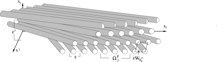
Figure 4.1. Non-periodic plywood-structure

We would like to study elastic properties of a exoskeleton. In the formulation of the microscopic model defined on the scale of a single fibre, we shall distinguish between mechanical properties of fibres and inter-fibrous space. We assume that the fibres are cylinders of radius $\varepsilon a$, perpendicular to the $x_{3}$-axis, whereas $0<a<1/2$ and $\varepsilon>0$. It has been observed that different parts of the exoskeleton comprise different rotation densities, [15]. Thus, we shall distinguish between the locally-periodic plywood structure, where the hight of layers of fibres aligned in the same direction is of order $\varepsilon^{r}$ with $0<r<1$, and the non-periodic microstructure, where each layer of fibres is rotated by a different angle, i.e. $r=1$, see Fig. 2.1 and Fig. 4.1 in Section 4. In the derivation of effective macroscopic equations the non-periodic situation shall be approximated by the locally-periodic microstructure. The case $r=0$ would imply the periodic microstructure and will not be considered here.

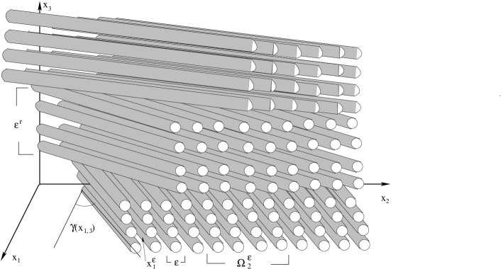
Figure 2.1. Locally-periodic plywood structure.

In order to define the characteristic function of the domain occupied by fibres for locally-periodic plywood structure we divide $\mathbb{R}^{3}$ into perpendicular to the $x_{3}$-axis layers $L_{k}^{\varepsilon}=\mathbb{R}^{2}\times((k-1)\varepsilon^{r},k\varepsilon^{r})$ of height $\varepsilon^{r}$, where $k\in\mathbb{Z}$ and $0<r<1$, and in each $L_{k}^{\varepsilon}$ choose an arbitrary point $x_{k}^{\varepsilon}\in L_{k}^{\varepsilon}$. In $\mathbb{R}\times\hat{Y}$, with $\hat{Y}=[0,1]^{2}$, we consider the characteristic function $\tilde{\eta}$ of a cylinder of radius $a$

(2.1) $$\tilde{\eta}(y)=\begin{cases}1,\quad|\hat{y}-1/2|\leq a,\\ 0,\quad|\hat{y}-1/2|>a,\end{cases}$$

where $\hat{y}=(y_{2},y_{3})$, and extended $\hat{Y}$-periodically to the whole of $\mathbb{R}^{3}$.

For a Lipschitz bounded domain $\Omega$ we define $\Omega_{f}^{\varepsilon}\subset\Omega$ as the subdomain occupied by fibres. Then the characteristic function of $\Omega^{\varepsilon}_{f}$ is given by

(2.2) $$\chi_{\Omega_{f}^{\varepsilon}}(x)=\chi_{\Omega}(x)\sum\limits_{k\in\mathbb{Z}}\eta_{\varepsilon}(R_{x_{k}^{\varepsilon}}\,x)\chi_{L_{k}^{\varepsilon}}(x),$$

with $\eta_{\varepsilon}(x)=\eta(x/\varepsilon)$ and $R_{x_{k}^{\varepsilon}}=R(\gamma(x_{k,3}^{\varepsilon}))$, where $\gamma\in C^{2}(\mathbb{R})$ is a given function, $0\leq\gamma(x)\leq\pi$ for $x\in\mathbb{R}$, and $R(\alpha)$ is the inverse of the rotation matrix around the $x_{3}$-axis with rotation angle $\alpha$ with the $x_{1}$-axis

$$R(\alpha)=\left(\begin{array}[]{ccc}\phantom{-}\cos(\alpha)&\sin(\alpha)&0\\ -\sin(\alpha)&\cos(\alpha)&0\\ 0&0&1\end{array}\right).$$

The assumed regularity of $\gamma$ will be essential for the homogenization analysis in Section 4. By $\chi_{A}$ we denote the characteristic function of a domain $A$.

In the context of the theory of linear elasticity, which is widely used in the continuous mechanics of solid materials, [17], we describe the elastic properties of a material with the plywood structure

(2.3) $$\begin{cases}-\text{div}\left(E^{\varepsilon}(x)\,e(u^{\varepsilon})\right)=G\quad&\text{ in }\Omega,\\ u^{\varepsilon}=g\qquad&\text{ on }\partial\Omega,\end{cases}$$

where $e_{ij}(u^{\varepsilon})=\frac{1}{2}\left(\frac{\partial u^{\varepsilon}_{i}}{\partial x_{j}}+\frac{\partial u^{\varepsilon}_{j}}{\partial x_{i}}\right)$ and the elasticity tensor $E^{\varepsilon}$ is given by

(2.4) $$E^{\varepsilon}(x)=E_{1}\chi_{\Omega_{f}^{\varepsilon}}(x)+E_{2}\big{(}1-\chi_{\Omega_{f}^{\varepsilon}}(x)).$$

Here $E_{1}$ is the stiffness tensor of the chitin-protein fibres and $E_{2}$ is the stiffness tensor of the inter-fibre space. The boundary condition and the right hand side describe the external forces applied to the material.

The considered microstructure is locally-periodic, i.e. it is periodic in each layer $L_{k}^{\varepsilon}$, where the height of the layer $\varepsilon^{r}$ is larger as the radius of a single fibre, but is small compared to the size of the considered domain $\Omega$, provide $\varepsilon$ is sufficiently small.

To allow more general locally-periodic oscillations and microstructures, we shall consider the partition of $\Omega$ into cubes of side $\varepsilon^{r}$ in the definition of the locally-periodic two-scale convergence. In the locally-periodic plywood-structure the rotation angle is constant in each layer $L_{k}^{\varepsilon}$ and the characteristic function of $\Omega^{\varepsilon}_{f}$ can also be defined considering the additional division of $L_{k}^{\varepsilon}$ into cubes of side $\varepsilon^{r}$. Thus, the introduced below locally-periodic two-scale convergence is applicable to fibrous media. Although the division of $\Omega$ into layers $L_{k}^{\varepsilon}$ is sufficient to define the microstructure of the locally periodic plywood-structure, for the homogenization of a non-periodic plywood-structure the partition covering of $\Omega$ by cubes will be essential, see Section 4.

3. Two-scale convergence for locally-periodic microstructures

First we introduce the space-dependent periodicity and the corresponding function spaces. Let $\Omega\subset\mathbb{R}^{d}$ be a bounded Lipschitz domain. For each $x\in\mathbb{R}^{d}$ we consider a transformation matrix $D(x)\in\mathbb{R}^{d\times d}$ and its inverse $D^{-1}(x)$, such that $D,D^{-1}\in\text{Lip}(\mathbb{R}^{d};\mathbb{R}^{d\times d})$ and $0<D_{1}\leq|\det D(x)|\leq D_{2}<\infty$ for all $x\in\overline{\Omega}$. For convenience, we shall use the notations $D_{x}:=D(x)$ and $D_{x}^{-1}:=D^{-1}(x)$. By $Y=[0,1]^{d}$ we denote the so-called ’unit cell’ and consider the continuous family of parallelepipeds $Y_{x}=D_{x}Y$ on $\overline{\Omega}$.

We shall consider the space $C(\overline{\Omega};C_{\text{per}}(Y_{x}))$ given in a standard way, i.e. for any $\tilde{\psi}\in C(\overline{\Omega};C_{\text{per}}(Y))$ the relation $\psi(x,y)=\tilde{\psi}(x,D_{x}^{-1}y)$ with $x\in\Omega$ and $y\in Y_{x}$ yields $\psi\in C(\overline{\Omega};C_{\text{per}}(Y_{x}))$. In the same way the spaces $L^{p}(\Omega;C_{\text{per}}(Y_{x}))$, $L^{p}(\Omega;L^{q}_{\text{per}}(Y_{x}))$ and $C(\overline{\Omega};L^{q}_{\text{per}}(Y_{x}))$, for $1\leq p\leq\infty$, $1\leq q<\infty$, are given.

The separability of $C_{\text{per}}(Y_{x})$ for each $x\in\Omega$ and the Weierstrass approximation for continuous functions $u\in(\Omega\to C_{\text{per}}(Y_{x}))$ imply the separability of $C(\overline{\Omega};C_{\text{per}}(Y_{x}))$. For the norm $\|\psi\|_{C(\overline{\Omega};C_{\text{per}}(Y_{x}))}:=\sup\limits_{x\in\overline{\Omega}}\sup\limits_{y\in Y_{x}}|\psi(x,y)|$ we have the relations

$$\|\psi\|_{C(\overline{\Omega};C_{\text{per}}(Y_{x}))}=\sup\limits_{x\in\overline{\Omega}}\sup\limits_{y\in Y_{x}}|\tilde{\psi}(x,D_{x}^{-1}y)|=\sup\limits_{x\in\overline{\Omega}}\sup\limits_{\tilde{y}\in Y}|\tilde{\psi}(x,\tilde{y})|.$$

For $p<\infty$, the separability of $C_{\text{per}}(Y_{x})$ for $x\in\Omega$ and the approximation of $L^{p}$- functions $u\in(\Omega\to C_{\text{per}}(Y_{x}))$ by simple functions imply the separability of $L^{p}(\Omega;C_{\text{per}}(Y_{x}))$. The norm is defined in the standard way

$$\|\psi\|_{L^{p}(\Omega;C_{\text{per}}(Y_{x}))}:=\int_{\Omega}\sup\limits_{y\in Y_{x}}|\psi(x,y)|^{p}\,dx.$$

The space $L^{2}(\Omega;L^{2}(Y_{x}))$ is a Hilbert space with a scalar product given by

$$\int_{\Omega}\int_{Y_{x}}\psi(x,y)\phi(x,y)\,dydx=\int_{\Omega}\int_{Y}\tilde{\psi}(x,\tilde{y})\tilde{\phi}(x,\tilde{y})|\det D_{x}|d\tilde{y}dx$$

for $\psi,\phi\in L^{2}(\Omega;L^{2}(Y_{x}))$ with $\psi(x,y)=\tilde{\psi}(x,D_{x}^{-1}y)$, $\phi(x,y)=\tilde{\phi}(x,D_{x}^{-1}y)$ for a.a $x\in\Omega$ and $y\in Y_{x}$, and $\tilde{\psi},\tilde{\phi}\in L^{2}(\Omega;L^{2}(Y))$.

Due to the assumptions on $D$, i.e. $D\in\text{Lip}(\overline{\Omega})$ and $|\det D(x)|$ is uniformly bounded from below and above in $\overline{\Omega}$, we obtain that

$$L^{2}(\Omega;H^{1}(Y_{x})) = \{u\in L^{2}(\Omega;L^{2}(Y_{x})),\,\nabla_{y}u\in L^{2}(\Omega;L^{2}(Y_{x})^{d})\}\quad\qquad\text{ and }$$

$$L^{2}(\Omega;L^{2}(\partial Y_{x})) = \Big{\{}u:\cup_{x\in\Omega}\big{(}\{x\}\times\partial Y_{x}\big{)}\to\mathbb{R}\text{ measurable},\int_{\Omega}\|u\|^{2}_{L^{2}(\partial Y_{x})}dx<\infty\Big{\}}$$

are well-defined, separable Hilbert spaces, [14, 22, 33].

To introduce the notion of locally-periodic two-scale convergence for a sequence $\{u^{\varepsilon}\}_{\varepsilon>0}$ in $L^{2}(\Omega)$ we consider the covering of $\Omega$ by cubes. For $\varepsilon>0$, similarly as in [11], we consider the partition covering of $\Omega$ by a family of open non-intersecting cubes $\{\Omega_{n}^{\varepsilon}\}_{1\leq n\leq N_{\varepsilon}}$ of side $\varepsilon^{r}$, with $0<r<1$, such that

$$\Omega\subset\cup_{n=1}^{N_{\varepsilon}}\overline{\Omega}_{n}^{\varepsilon}\quad\text{and }\quad\Omega_{n}^{\varepsilon}\cap\Omega\neq\emptyset,$$

where $N_{\varepsilon}$ is the number of $\Omega_{n}^{\varepsilon}$ having a non-empty intersection with $\Omega$. We consider

$$\mathcal{K}^{\varepsilon}=\Omega\setminus\big{(}\cup_{n=1}^{\tilde{N}_{\varepsilon}}\overline{\Omega}_{n}^{\varepsilon}\big{)},$$

where by $\tilde{N}_{\varepsilon}$ we denote the number of all cubes $\Omega_{n}^{\varepsilon}$ enclosed in $\Omega$. Then

$$\mathcal{K}^{\varepsilon}\subset\cup_{n=\tilde{N}_{\varepsilon}+1}^{N_{\varepsilon}}\overline{\Omega}_{n}^{\varepsilon}.$$

All $\Omega_{n}^{\varepsilon}$ with $n=\tilde{N}_{\varepsilon}+1,\ldots,N_{\varepsilon}$ have the non-empty intersection with $\partial\Omega$ and are enclosed in a $\varepsilon^{r}$-neighbourhood of $\partial\Omega$. Then the size of the domain $\mathcal{K}^{\varepsilon}$ can be estimated

$$|\mathcal{K}^{\varepsilon}|\leq C\varepsilon^{r},$$

with some constant $C$. This gives $\tilde{N}_{\varepsilon}\varepsilon^{rd}\leq|\Omega|$ and $N_{\varepsilon}\varepsilon^{rd}\leq|\Omega|+C$ for $\varepsilon\leq 1$. Thus

$$N_{\varepsilon}\leq C\varepsilon^{-rd}\quad\text{ and }\quad\tilde{N}_{\varepsilon}\leq C\varepsilon^{-rd}.$$

In the following we shall denote by $x_{n}^{\varepsilon},\tilde{x}_{n}^{\varepsilon}\in\Omega_{n}^{\varepsilon}\cap\Omega$, for $n=1,\ldots,N_{\varepsilon}$, arbitrary chosen fixed points.

We consider $\psi\in C(\overline{\Omega};C_{\text{per}}(Y_{x}))$ and corresponding function $\tilde{\psi}\in C(\overline{\Omega};C_{\text{per}}(Y))$. As a locally-periodic approximation of $\psi$ we name $\mathcal{L}^{\varepsilon}:C(\overline{\Omega};C_{\text{per}}(Y_{x}))\to L^{\infty}(\Omega)$ given by

$$(\mathcal{L}^{\varepsilon}\psi)(x)=\sum\limits_{n=1}^{N_{\varepsilon}}\tilde{\psi}\Big{(}x,\frac{D^{-1}_{x_{n}^{\varepsilon}}(x-\tilde{x}_{n}^{\varepsilon})}{\varepsilon}\Big{)}\chi_{\Omega_{n}^{\varepsilon}}(x)\quad\text{ for }x\in\Omega.$$

We consider also the map $\mathcal{L}^{\varepsilon}_{0}:C(\overline{\Omega};C_{\text{per}}(Y_{x}))\to L^{\infty}(\Omega)$ defined for $x\in\Omega$ as

$$(\mathcal{L}^{\varepsilon}_{0}\psi)(x)=\sum\limits_{n=1}^{N_{\varepsilon}}\psi\Big{(}x_{n}^{\varepsilon},\frac{x-\tilde{x}_{n}^{\varepsilon}}{\varepsilon}\Big{)}\chi_{\Omega_{n}^{\varepsilon}}(x)=\sum\limits_{n=1}^{N_{\varepsilon}}\tilde{\psi}\Big{(}x_{n}^{\varepsilon},\frac{D^{-1}_{x_{n}^{\varepsilon}}(x-\tilde{x}_{n}^{\varepsilon})}{\varepsilon}\Big{)}\chi_{\Omega_{n}^{\varepsilon}}(x).$$

If we choose $\tilde{x}_{n}^{\varepsilon}=D_{x_{n}^{\varepsilon}}\varepsilon k$ for some $k\in\mathbb{Z}^{d}$, then the periodicity of $\tilde{\psi}$ implies

$$(\mathcal{L}^{\varepsilon}\psi)(x)=\sum\limits_{n=1}^{N_{\varepsilon}}\tilde{\psi}\Big{(}x,\frac{D^{-1}_{x_{n}^{\varepsilon}}x}{\varepsilon}\Big{)}\chi_{\Omega_{n}^{\varepsilon}}(x)\quad\text{ and }\quad(\mathcal{L}^{\varepsilon}_{0}\psi)(x)=\sum\limits_{n=1}^{N_{\varepsilon}}\tilde{\psi}\Big{(}x_{n}^{\varepsilon},\frac{D^{-1}_{x_{n}^{\varepsilon}}x}{\varepsilon}\Big{)}\chi_{\Omega_{n}^{\varepsilon}}(x)$$

for $x\in\Omega$. In following we shall consider the case $\tilde{x}_{n}^{\varepsilon}=D_{x_{n}^{\varepsilon}}\varepsilon k$, with $k\in\mathbb{Z}^{d}$, however all results hold for arbitrary chosen $\tilde{x}_{n}^{\varepsilon}\in\Omega_{n}^{\varepsilon}$ with $n=1,\ldots,N_{\varepsilon}$.
In the similar way we define $\mathcal{L}^{\varepsilon}\psi$ and $\mathcal{L}^{\varepsilon}_{0}\psi$ for $\psi$ in $C(\overline{\Omega};L^{q}_{\text{per}}(Y_{x}))$ or $L^{p}(\Omega;C_{\text{per}}(Y_{x}))$.
In the proof of convergence theorem we shall use the regular approximation of $\mathcal{L}^{\varepsilon}\psi$

$$(\mathcal{L}^{\varepsilon}_{\rho}\psi)(x)=\sum\limits_{n=1}^{N_{\varepsilon}}\tilde{\psi}\Big{(}x,\frac{D^{-1}_{x_{n}^{\varepsilon}}x}{\varepsilon}\Big{)}\phi_{\Omega_{n}^{\varepsilon}}(x)\quad\text{ for }x\in\Omega,$$

where $\phi_{\Omega_{n}^{\varepsilon}}$ are approximations of $\chi_{\Omega_{n}^{\varepsilon}}$ such that $\phi_{\Omega_{n}^{\varepsilon}}\in C^{\infty}_{0}(\Omega_{n}^{\varepsilon})$ and

(3.1) $$\sum\limits_{n=1}^{N_{\varepsilon}}|\phi_{\Omega_{n}^{\varepsilon}}-\chi_{\Omega_{n}^{\varepsilon}}|\to 0\,\text{ in }L^{2}(\Omega),\,\,||\nabla^{m}\phi_{\Omega_{n}^{\varepsilon}}||_{L^{\infty}(\mathbb{R}^{d})}\leq C\varepsilon^{-\rho m}\,\text{ for }0<r<\rho<1.$$

We can consider $\phi_{\Omega_{n}^{\varepsilon}}(x)=\varphi_{\varepsilon}\ast\chi_{\Omega_{n,\rho}^{\varepsilon}}$ for $\Omega_{n}^{\varepsilon}\subset\Omega$ and $\phi_{\Omega_{n}^{\varepsilon}}(x)=0$ for $\Omega_{n}^{\varepsilon}\cap\partial\Omega\neq\emptyset$, where $\varphi_{\varepsilon}(x)=\frac{1}{\varepsilon^{n\rho}}\varphi(\frac{x}{\varepsilon^{\rho}})$, with $\varphi(x)=c\exp(-1/(1-|x|^{2}))$ for $|x|<1$ and $\varphi(x)=0$ for $|x|\geq 1$ and $\Omega_{n,\rho}^{\varepsilon}=\{x\in\Omega_{n}^{\varepsilon},\text{dist}(x,\partial\Omega_{n}^{\varepsilon})>\varepsilon^{\rho}\}$. The constant $c$ is such that $\int_{\mathbb{R}^{d}}\varphi(x)dx=1$. Then $\phi_{\Omega_{n}^{\varepsilon}}\in C^{\infty}_{0}(\Omega_{n}^{\varepsilon})$ and (3.1) follow from the properties of $\varphi_{\varepsilon}$. Notice that $\|\sum_{n=1}^{N_{\varepsilon}}|\phi_{\Omega_{n}^{\varepsilon}}-\chi_{\Omega_{n}^{\varepsilon}}|\|_{L^{2}(\Omega)}\leq c_{1}\varepsilon^{r(d-1)}\varepsilon^{\rho}N_{\varepsilon}\leq c_{2}\varepsilon^{\rho-r}.$
Another construction of $\phi_{\Omega_{n}^{\varepsilon}}$ can be found in [9].

Example. Let $\Omega=(0,1)$, $Y=[0,1]$, and the family of cubes $\Omega_{n}^{\varepsilon}=(n-1,n)\varepsilon^{r}$ with $\varepsilon=N^{-1/r}$ for some $N\in\mathbb{N}$, and $n=1,\ldots,N_{\varepsilon}$, where $N_{\varepsilon}=N=\varepsilon^{-r}$. With $D(x)=e^{x}$ for $x\in\overline{\Omega}$ we obtain the family of intervals $Y_{x}=[0,e^{x}]$. We consider $\psi(x,y)=x+\sin(2\pi e^{-x}y)$ in $C(\overline{\Omega};C_{\text{per}}(Y_{x}))$ and corresponding $\tilde{\psi}(x,\tilde{y})=x+\sin(2\pi\tilde{y})$ in $C(\overline{\Omega};C_{\text{per}}(Y))$. Then the locally-periodic approximation of $\psi$ is given by $\mathcal{L}^{\varepsilon}\psi(x)=\sum_{n=1}^{N_{\varepsilon}}\left(x+\sin(2\pi e^{-x_{n}^{\varepsilon}}x/\varepsilon)\right)\chi_{\Omega_{n}^{\varepsilon}}(x)$, with e.g. $x_{n}^{\varepsilon}=(n-1/2)\varepsilon^{r}$, and $\mathcal{L}^{\varepsilon}_{0}\psi(x)=\sum_{n=1}^{N_{\varepsilon}}\left(x_{n}^{\varepsilon}+\sin(2\pi e^{-x_{n}^{\varepsilon}}x/\varepsilon)\right)\chi_{\Omega_{n}^{\varepsilon}}(x)$.

Definition 1.

Let $u^{\varepsilon}\in L^{2}(\Omega)$ for all $\varepsilon>0$. We say the sequence $\{u^{\varepsilon}\}$ converges locally-periodic two-scale (l-t-s) to $u\in L^{2}(\Omega;L^{2}(Y_{x}))$ as $\varepsilon\to 0$ if for any $\psi\in L^{2}(\Omega;C_{\text{per}}(Y_{x}))$

$$\lim\limits_{\varepsilon\to 0}\int_{\Omega}u^{\varepsilon}(x)\mathcal{L}^{\varepsilon}\psi(x)dx=\int_{\Omega}\mathchoice{{\vbox{\hbox{$\textstyle-$}}\kern-5.05557pt}}{{\vbox{\hbox{$\scriptstyle-$}}\kern-3.38004pt}}{{\vbox{\hbox{$\scriptscriptstyle-$}}\kern-2.38335pt}}{{\vbox{\hbox{$\scriptscriptstyle-$}}\kern-1.95001pt}}\!\int_{Y_{x}}u(x,y)\psi(x,y)dydx,$$

where $\mathcal{L}^{\varepsilon}\psi$ is the locally-periodic approximation of $\psi$.

Notice that taking in the Definition 1 a test function $\psi$ independent of $y$ yields

$$u^{\varepsilon}(x)\rightharpoonup\mathchoice{{\vbox{\hbox{$\textstyle-$}}\kern-5.05557pt}}{{\vbox{\hbox{$\scriptstyle-$}}\kern-3.38004pt}}{{\vbox{\hbox{$\scriptscriptstyle-$}}\kern-2.38335pt}}{{\vbox{\hbox{$\scriptscriptstyle-$}}\kern-1.95001pt}}\!\int_{Y_{x}}u(x,y)dy\quad\text{ in }\quad L^{2}(\Omega).$$

The subsequent convergence results for the locally-periodic approximation will ensure that Definition 1 does not depend on the choice of $x_{n}^{\varepsilon},\tilde{x}_{n}^{\varepsilon}\in\Omega_{n}^{\varepsilon}$ for $n=1,\ldots,N_{\varepsilon}$.

The main results of this section are the compactness theorem for the locally-periodic two-scale convergence and the characterisation of the locally-periodic two-scale limit for a sequence bounded in $H^{1}(\Omega)$.

Theorem 2.

Let $\{u^{\varepsilon}\}$ be a bounded sequence in $L^{2}(\Omega)$. Then there exists a subsequence of $\{u^{\varepsilon}\}$, denoted again by $\{u^{\varepsilon}\}$, and a function $u\in L^{2}(\Omega;L^{2}(Y_{x}))$, such that $u^{\varepsilon}\to u$ in the locally-periodic two-scale sense as $\varepsilon\to 0$.

Theorem 3.

Let $\{u^{\varepsilon}\}$ be a bounded sequence in $H^{1}(\Omega)$ that converges weakly to $u$ in $H^{1}(\Omega)$. Then

• the sequence $\{u^{\varepsilon}\}$ converges locally-periodic two-scale to $u$;

• there exist a subsequence of $\{\nabla u^{\varepsilon}\}$, denoted again by $\{\nabla u^{\varepsilon}\}$, and a function $u_{1}\in L^{2}(\Omega;H^{1}_{\text{per}}(Y_{x})/\mathbb{R})$ such that $\nabla u^{\varepsilon}\to\nabla u+\nabla_{y}u_{1}$ in the locally-periodic two-scale sense as $\varepsilon\to 0$.

The proofs of the main results rely on some convergence results for locally-periodic approximations of $Y_{x}$-periodic functions.

Lemma 4.

For $\psi\in L^{p}(\Omega;C_{\text{per}}(Y_{x}))$, with $1\leq p<\infty$, we have

(3.2) $$\lim\limits_{\varepsilon\to 0}\int_{\Omega}\left|\mathcal{L}^{\varepsilon}\psi(x)\right|^{p}dx=\int_{\Omega}\,\mathchoice{{\vbox{\hbox{$\textstyle-$}}\kern-5.05557pt}}{{\vbox{\hbox{$\scriptstyle-$}}\kern-3.38004pt}}{{\vbox{\hbox{$\scriptscriptstyle-$}}\kern-2.38335pt}}{{\vbox{\hbox{$\scriptscriptstyle-$}}\kern-1.95001pt}}\!\int_{Y_{x}}|\psi(x,y)|^{p}dy\,dx$$

and for $\psi\in L^{1}(\Omega;C_{\text{per}}(Y_{x}))$ we obtain

(3.3) $$\lim\limits_{\varepsilon\to 0}\int_{\Omega}\mathcal{L}^{\varepsilon}\psi(x)dx=\int_{\Omega}\,\mathchoice{{\vbox{\hbox{$\textstyle-$}}\kern-5.05557pt}}{{\vbox{\hbox{$\scriptstyle-$}}\kern-3.38004pt}}{{\vbox{\hbox{$\scriptscriptstyle-$}}\kern-2.38335pt}}{{\vbox{\hbox{$\scriptscriptstyle-$}}\kern-1.95001pt}}\!\int_{Y_{x}}\psi(x,y)dy\,dx.$$

For $\psi\in C(\overline{\Omega};L^{p}_{\text{per}}(Y_{x}))$, where $1\leq p<\infty$, we have

(3.4) $$\lim\limits_{\varepsilon\to 0}\int_{\Omega}\,\left|\mathcal{L}^{\varepsilon}_{0}\psi(x)\right|^{p}dx=\int_{\Omega}\,\mathchoice{{\vbox{\hbox{$\textstyle-$}}\kern-5.05557pt}}{{\vbox{\hbox{$\scriptstyle-$}}\kern-3.38004pt}}{{\vbox{\hbox{$\scriptscriptstyle-$}}\kern-2.38335pt}}{{\vbox{\hbox{$\scriptscriptstyle-$}}\kern-1.95001pt}}\!\int_{Y_{x}}|\psi(x,y)|^{p}dy\,dx$$

and for $\psi\in C(\overline{\Omega};L^{1}_{\text{per}}(Y_{x}))$ we obtain

(3.5) $$\lim\limits_{\varepsilon\to 0}\int_{\Omega}\,\mathcal{L}^{\varepsilon}_{0}\psi(x)dx=\int_{\Omega}\,\mathchoice{{\vbox{\hbox{$\textstyle-$}}\kern-5.05557pt}}{{\vbox{\hbox{$\scriptstyle-$}}\kern-3.38004pt}}{{\vbox{\hbox{$\scriptscriptstyle-$}}\kern-2.38335pt}}{{\vbox{\hbox{$\scriptscriptstyle-$}}\kern-1.95001pt}}\!\int_{Y_{x}}\psi(x,y)dy\,dx.$$

If $\psi\in L^{p}(\overline{\Omega};C^{1}_{\text{per}}(Y_{x}))$, with $1\leq p<\infty$, then we have

(3.6) $$\lim\limits_{\varepsilon\to 0}\int_{\Omega}\,\left|\mathcal{L}^{\varepsilon}\nabla_{y}\psi(x)\right|^{p}dx=\int_{\Omega}\,\mathchoice{{\vbox{\hbox{$\textstyle-$}}\kern-5.05557pt}}{{\vbox{\hbox{$\scriptstyle-$}}\kern-3.38004pt}}{{\vbox{\hbox{$\scriptscriptstyle-$}}\kern-2.38335pt}}{{\vbox{\hbox{$\scriptscriptstyle-$}}\kern-1.95001pt}}\!\int_{Y_{x}}|\nabla_{y}\psi(x,y)|^{p}dydx.$$

Proof.

We start with the proof of (3.2) for $\psi\in C(\overline{\Omega};C_{\text{per}}(Y_{x}))$. The translations of $Y=[0,1]^{d}$ are given by $Y^{i}=Y+k_{i}$ with $k_{i}\in\mathbb{Z}^{d}$. Then for $x_{n}^{\varepsilon}\in\Omega_{n}^{\varepsilon}$ and $D_{x_{n}^{\varepsilon}}=D(x_{n}^{\varepsilon})$ we consider $Y_{x_{n}^{\varepsilon}}^{i}=D_{x_{n}^{\varepsilon}}Y^{i}$, obtained by the linear transformation of $Y^{i}$, and cover $\Omega_{n}^{\varepsilon}$, with $1\leq n\leq N_{\varepsilon}$, by the family of closed parallelepipeds $\{\varepsilon Y_{x_{n}^{\varepsilon}}^{i}\}_{i=1}^{I_{n}^{\varepsilon}}$:

$$\Omega_{n}^{\varepsilon}\subset\cup_{i=1}^{I_{n}^{\varepsilon}}\varepsilon Y_{x_{n}^{\varepsilon}}^{i}\quad\text{ such that }\,\,\varepsilon Y_{x_{n}^{\varepsilon}}^{i}\cap\overline{\Omega}_{n}^{\varepsilon}\neq\emptyset,$$

where $I_{n}^{\varepsilon}$ is the number of parallelepipeds covering $\Omega_{n}^{\varepsilon}$. The domain $\mathcal{M}_{n}^{\varepsilon}$ given by

$$\mathcal{M}_{n}^{\varepsilon}=\Omega_{n}^{\varepsilon}\setminus\Big{(}\cup_{i=1}^{\tilde{I}_{n}^{\varepsilon}}\varepsilon Y_{x_{n}^{\varepsilon}}^{i}\Big{)},$$

with $\tilde{I}_{n}^{\varepsilon}$ as the number of all $\varepsilon Y_{x_{n}^{\varepsilon}}^{i}$ enclosed in $\Omega_{n}^{\varepsilon}$, satisfies $\mathcal{M}_{n}^{\varepsilon}\subset\cup_{i=\tilde{I}_{n}^{\varepsilon}+1}^{I_{n}^{\varepsilon}}\varepsilon Y_{x_{n}^{\varepsilon}}^{i}.$ All $\varepsilon Y_{x_{n}^{\varepsilon}}^{i}$, for $i=\tilde{I}_{n}^{\varepsilon}+1,\ldots,I_{n}^{\varepsilon}$, have the non-empty intersection with $\partial\Omega_{n}^{\varepsilon}$ and are enclosed in a $\varepsilon$-neighbourhood of $\partial\Omega_{n}^{\varepsilon}$. This ensures the estimate

$$|\mathcal{M}_{n}^{\varepsilon}|\leq C_{1}|\partial\Omega_{n}^{\varepsilon}|\varepsilon\leq C_{2}\,\varepsilon^{(d-1)r+1}\qquad\,\text{ for all }\,\,n=1,\ldots,N_{\varepsilon}.$$

Thus we have $\varepsilon^{d}|\det D_{x_{n}^{\varepsilon}}|\tilde{I}_{n}^{\varepsilon}\leq\varepsilon^{dr}$ and $\varepsilon^{d}|\det D_{x_{n}^{\varepsilon}}|I_{n}^{\varepsilon}\leq C\varepsilon^{dr}$ for $\varepsilon\leq 1$, i.e.

$$\tilde{I}_{n}^{\varepsilon}\leq C\varepsilon^{d(r-1)}\quad\text{ and }\quad I_{n}^{\varepsilon}\leq C\varepsilon^{d(r-1)}\quad\text{ for all }\,\,n=1,\ldots,N_{\varepsilon}.$$

Considering the covering of $\Omega_{n}^{\varepsilon}$, we rewrite the integral on the left hand side of (3.2)

$$\int_{\Omega}\left|\mathcal{L}^{\varepsilon}\psi(x)\right|^{p}dx = \sum\limits_{n=1}^{\tilde{N}_{\varepsilon}}\sum\limits_{i=1}^{\tilde{I}_{n}^{\varepsilon}}\int_{\varepsilon Y_{x_{n}^{\varepsilon}}^{i}}\Big{|}\tilde{\psi}\Big{(}x_{n}^{\varepsilon},\frac{D^{-1}_{x_{n}^{\varepsilon}}x}{\varepsilon}\Big{)}\Big{|}^{p}dx$$

$$+ \sum\limits_{n=1}^{\tilde{N}_{\varepsilon}}\sum\limits_{i=1}^{\tilde{I}_{n}^{\varepsilon}}\int_{\varepsilon Y_{x_{n}^{\varepsilon}}^{i}}\Big{(}\Big{|}\tilde{\psi}\Big{(}x,\frac{D^{-1}_{x_{n}^{\varepsilon}}x}{\varepsilon}\Big{)}\Big{|}^{p}-\Big{|}\tilde{\psi}\Big{(}x_{n}^{\varepsilon},\frac{D^{-1}_{x_{n}^{\varepsilon}}x}{\varepsilon}\Big{)}\Big{|}^{p}\Big{)}dx$$

$$+ \sum\limits_{n=1}^{\tilde{N}_{\varepsilon}}\int_{\mathcal{M}_{n}^{\varepsilon}}\Big{|}\tilde{\psi}\Big{(}x,\frac{D^{-1}_{x_{n}^{\varepsilon}}x}{\varepsilon}\Big{)}\Big{|}^{p}dx+\int_{\mathcal{K}^{\varepsilon}}\left|\mathcal{L}^{\varepsilon}\psi(x)\right|^{p}dx=I_{1}+I_{2}+I_{3}+I_{4}.$$

Applying the inequality $||a|^{p}-|b|^{p}|\leq p(|a|^{p-1}+|b|^{p-1})|a-b|$, see [4], the assumptions on $D$, the continuity $\psi$, the bounds for $\tilde{N}_{\varepsilon}$ and $\tilde{I}_{n}^{\varepsilon}$, and the property

$$\sup\limits_{1\leq i\leq\tilde{I}_{n}^{\varepsilon}}\sup\limits_{x\in\varepsilon Y_{x_{n}^{\varepsilon}}^{i}}|x-x_{n}^{\varepsilon}|\leq C\varepsilon^{r},$$

ensured by the fact that $|\Omega_{n}^{\varepsilon}|=\varepsilon^{r}$ for all $1\leq n\leq N_{\varepsilon}$, we can estimate $I_{2}$ by

(3.7) $$2p\|\psi\|_{C(\overline{\Omega},C_{\text{per}}(Y_{x}))}^{p-1}\sum\limits_{n=1}^{\tilde{N}_{\varepsilon}}\sum\limits_{i=1}^{\tilde{I}_{n}^{\varepsilon}}|\varepsilon Y_{x_{n}^{\varepsilon}}^{i}|\sup\limits_{x\in\varepsilon Y_{x_{n}^{\varepsilon}}^{i}}\sup\limits_{\tilde{y}\in Y}|\tilde{\psi}(x,\tilde{y})-\tilde{\psi}(x_{n}^{\varepsilon},\tilde{y})|\leq C\delta_{1}(\varepsilon)|\Omega|,$$

where $\delta_{1}(\varepsilon)\to 0$ as $\varepsilon\to 0$. For $I_{3}$ and $I_{4}$ the regularity of $\psi$ together with the bounds for $|\mathcal{K}^{\varepsilon}|$, $|\mathcal{M}_{n}^{\varepsilon}|$, and $\tilde{N}_{\varepsilon}$ implies

(3.8) $$|I_{3}|+|I_{4}|\leq\|\psi(x,y)\|_{C(\overline{\Omega},C_{\text{per}}(Y_{x}))}^{p}\Big{(}\sum\limits_{n=1}^{\tilde{N}_{\varepsilon}}|\mathcal{M}_{n}^{\varepsilon}|+|\mathcal{K}^{\varepsilon}|\Big{)}\leq C(\varepsilon^{1-r}+\varepsilon^{r}).$$

Combining now (3.7) and (3.8) gives

$$\qquad\int_{\Omega}\left|\mathcal{L}^{\varepsilon}\psi(x)\right|^{p}dx = \sum\limits_{n=1}^{\tilde{N}_{\varepsilon}}\tilde{I}_{n}^{\varepsilon}\varepsilon^{d}|\det D_{x_{n}^{\varepsilon}}|\int_{Y}|\tilde{\psi}(x_{n}^{\varepsilon},\tilde{y})|^{p}d\tilde{y}+\delta(\varepsilon)$$

$$= \int_{\Omega}\sum\limits_{n=1}^{\tilde{N}_{\varepsilon}}\mathchoice{{\vbox{\hbox{$\textstyle-$}}\kern-5.05557pt}}{{\vbox{\hbox{$\scriptstyle-$}}\kern-3.38004pt}}{{\vbox{\hbox{$\scriptscriptstyle-$}}\kern-2.38335pt}}{{\vbox{\hbox{$\scriptscriptstyle-$}}\kern-1.95001pt}}\!\int_{Y_{x_{n}^{\varepsilon}}}|\psi(x_{n}^{\varepsilon},y)|^{p}dy\,\chi_{\Omega_{n}^{\varepsilon}}(x)\,dx-\sum\limits_{n=1}^{\tilde{N}_{\varepsilon}}|\mathcal{M}_{n}^{\varepsilon}|\mathchoice{{\vbox{\hbox{$\textstyle-$}}\kern-5.05557pt}}{{\vbox{\hbox{$\scriptstyle-$}}\kern-3.38004pt}}{{\vbox{\hbox{$\scriptscriptstyle-$}}\kern-2.38335pt}}{{\vbox{\hbox{$\scriptscriptstyle-$}}\kern-1.95001pt}}\!\int_{Y_{x_{n}^{\varepsilon}}}|\psi(x_{n}^{\varepsilon},y)|^{p}dy+\delta(\varepsilon),$$

where $\delta(\varepsilon)\to 0$ as $\varepsilon\to 0$. The continuity of $\psi$ with respect to $x$ ensures

(3.10) $$\sum\limits_{n=1}^{\tilde{N}_{\varepsilon}}|\mathcal{M}_{n}^{\varepsilon}|\mathchoice{{\vbox{\hbox{$\textstyle-$}}\kern-5.05557pt}}{{\vbox{\hbox{$\scriptstyle-$}}\kern-3.38004pt}}{{\vbox{\hbox{$\scriptscriptstyle-$}}\kern-2.38335pt}}{{\vbox{\hbox{$\scriptscriptstyle-$}}\kern-1.95001pt}}\!\int_{Y_{x_{n}^{\varepsilon}}}|\psi(x_{n}^{\varepsilon},y)|^{p}dy\leq C_{1}\varepsilon^{1-r}\sup\limits_{x\in\Omega}\int_{Y}|\tilde{\psi}(x,\tilde{y})|^{p}d\tilde{y}\leq C_{2}\varepsilon^{1-r}.$$

Thus, the continuity of $F$, given by $F(x)=\mathchoice{{\vbox{\hbox{$\textstyle-$}}\kern-5.05557pt}}{{\vbox{\hbox{$\scriptstyle-$}}\kern-3.38004pt}}{{\vbox{\hbox{$\scriptscriptstyle-$}}\kern-2.38335pt}}{{\vbox{\hbox{$\scriptscriptstyle-$}}\kern-1.95001pt}}\!\int_{Y_{x}}|\psi(x,y)|^{p}dy$, in $\overline{\Omega}$ and the limit as $\varepsilon\to 0$ in (3) provide convergence (3.2) for $\psi\in C(\overline{\Omega};C_{\text{per}}(Y_{x}))$.

To prove (3.2) for $\psi\in L^{p}(\Omega;C_{\text{per}}(Y_{x}))$ we consider an approximation of $\psi$ by a sequence $\{\psi_{m}\}\subset C(\overline{\Omega};C_{\text{per}}(Y_{x}))$ such that $\psi_{m}\to\psi$ in $L^{p}(\Omega;C_{\text{per}}(Y_{x}))$. Using

$$\begin{array}[]{l}\left|\tilde{\psi}\Big{(}x,\frac{D^{-1}_{x_{n}^{\varepsilon}}x}{\varepsilon}\Big{)}\right|^{p}-\left|\tilde{\psi}_{m}\Big{(}x,\frac{D^{-1}_{x_{n}^{\varepsilon}}x}{\varepsilon}\Big{)}\right|^{p}=\left|\tilde{\psi}\Big{(}x,\frac{D^{-1}_{x}x}{\varepsilon}\Big{)}\right|^{p}-\left|\tilde{\psi}_{m}\Big{(}x,\frac{D^{-1}_{x}x}{\varepsilon}\Big{)}\right|^{p}\\ +\left|\tilde{\psi}\Big{(}x,\frac{D^{-1}_{x_{n}^{\varepsilon}}x}{\varepsilon}\Big{)}\right|^{p}-\left|\tilde{\psi}\Big{(}x,\frac{D^{-1}_{x}x}{\varepsilon}\Big{)}\right|^{p}+\left|\tilde{\psi}_{m}\Big{(}x,\frac{D^{-1}_{x}x}{\varepsilon}\Big{)}\right|^{p}-\left|\tilde{\psi}_{m}\Big{(}x,\frac{D^{-1}_{x_{n}^{\varepsilon}}x}{\varepsilon}\Big{)}\right|^{p}\end{array}$$

we obtain the following estimate

$$\int_{\Omega}\left|\left|\mathcal{L}^{\varepsilon}\psi(x)\right|^{p}-\left|\mathcal{L}^{\varepsilon}\psi_{m}(x)\right|^{p}\right|dx\leq\int_{\Omega}\sup\limits_{y\in Y_{x}}\left|\,|\psi(x,y)|^{p}-|\psi_{m}(x,y)|^{p}\right|dx$$

(3.11) $$\hskip 28.45274pt\qquad+\int_{\Omega}\sum\limits_{n=1}^{N_{\varepsilon}}\sup\limits_{\tilde{y}\in Y}\left|\left|\tilde{\psi}\left(x,\tilde{y}\right)\right|^{p}-\left|\tilde{\psi}\left(x,D^{-1}_{x}D_{x_{n}^{\varepsilon}}\tilde{y}\right)\right|^{p}\right|\chi_{\Omega_{n}^{\varepsilon}}(x)dx$$

$$\hskip 28.45274pt\qquad+\int_{\Omega}\sum\limits_{n=1}^{N_{\varepsilon}}\sup\limits_{\tilde{y}\in Y}\left|\left|\tilde{\psi}_{m}\left(x,\tilde{y}\right)\right|^{p}-\left|\tilde{\psi}_{m}\left(x,D^{-1}_{x}D_{x_{n}^{\varepsilon}}\tilde{y}\right)\right|^{p}\right|\chi_{\Omega_{n}^{\varepsilon}}(x)dx.$$

The inequality $||\psi|^{p}-|\psi_{m}|^{p}|\leq p(|\psi|^{p-1}+|\psi_{m}|^{p-1})|\psi-\psi_{m}|$, see [4], together with the Hölder inequality and the boundedness of $\psi_{m}$ and $\psi$ in $L^{p}(\Omega;C_{\text{per}}(Y_{x}))$ implies

$$\int_{\Omega}\sup\limits_{y\in Y_{x}}\left|\,|\psi|^{p}-|\psi_{m}|^{p}\right|dx\leq C\Big{(}\int_{\Omega}\sup\limits_{y\in Y_{x}}|\psi-\psi_{m}|^{p}dx\Big{)}^{\frac{1}{p}}.$$

The assumptions on $D$ and $\Omega^{\varepsilon}_{n}$ ensure $|\tilde{y}-D^{-1}_{x}D_{x_{n}^{\varepsilon}}\tilde{y}|\leq\delta_{2}(\varepsilon)$ for $x\in\Omega^{\varepsilon}_{n}$, $\tilde{y}\in Y$ and $n=1,\ldots,N_{\varepsilon}$, where $\delta_{2}(\varepsilon)\to 0$ as $\varepsilon\to 0$. Thus, using the continuity of $\psi$ and $\psi_{m}$ with respect to $y$, the convergence of $\psi_{m}$, and taking in (3) the limit as $\varepsilon\to 0$ and then as $m\to\infty$ we conclude

$$\lim\limits_{m\to\infty}\lim\limits_{\varepsilon\to 0}\int_{\Omega}\left(\left|\mathcal{L}^{\varepsilon}\psi(x)\right|^{p}-\left|\mathcal{L}^{\varepsilon}\psi_{m}(x)\right|^{p}\right)dx=0.$$

Applying now the calculations from above to $\psi_{m}\in C(\overline{\Omega};C_{\text{per}}(Y_{x}))$ for $m\in\mathbb{N}$ and considering the strong convergence of $\psi_{m}$ we obtain for $\psi\in L^{p}(\Omega;C_{\text{per}}(Y_{x}))$

$$\lim\limits_{\varepsilon\to 0}\int_{\Omega}\left|\mathcal{L}^{\varepsilon}\psi(x)\right|^{p}dx = \lim\limits_{m\to\infty}\lim\limits_{\varepsilon\to 0}\int_{\Omega}\left|\mathcal{L}^{\varepsilon}\psi_{m}(x)\right|^{p}dx$$

$$= \lim\limits_{m\to\infty}\int_{\Omega}\,\mathchoice{{\vbox{\hbox{$\textstyle-$}}\kern-5.05557pt}}{{\vbox{\hbox{$\scriptstyle-$}}\kern-3.38004pt}}{{\vbox{\hbox{$\scriptscriptstyle-$}}\kern-2.38335pt}}{{\vbox{\hbox{$\scriptscriptstyle-$}}\kern-1.95001pt}}\!\int_{Y_{x}}|\psi_{m}(x,y)|^{p}dy\,dx=\int_{\Omega}\,\mathchoice{{\vbox{\hbox{$\textstyle-$}}\kern-5.05557pt}}{{\vbox{\hbox{$\scriptstyle-$}}\kern-3.38004pt}}{{\vbox{\hbox{$\scriptscriptstyle-$}}\kern-2.38335pt}}{{\vbox{\hbox{$\scriptscriptstyle-$}}\kern-1.95001pt}}\!\int_{Y_{x}}|\psi(x,y)|^{p}dy\,dx.$$

The proof for (3.3) follows the same lines as for (3.2). First we consider $\psi\in C(\overline{\Omega};C_{\text{per}}(Y_{x}))$ and write the integral on the left hand side of (3.3) in the form

$$\int_{\Omega}\mathcal{L}^{\varepsilon}\psi(x)dx = \sum\limits_{n=1}^{\tilde{N}_{\varepsilon}}\sum\limits_{i=1}^{\tilde{I}_{n}^{\varepsilon}}\int_{\varepsilon Y_{x_{n}^{\varepsilon}}^{i}}\tilde{\psi}\Big{(}x_{n}^{\varepsilon},\frac{D^{-1}_{x_{n}^{\varepsilon}}x}{\varepsilon}\Big{)}+\Big{[}\tilde{\psi}\Big{(}x,\frac{D^{-1}_{x_{n}^{\varepsilon}}x}{\varepsilon}\Big{)}-\tilde{\psi}\Big{(}x_{n}^{\varepsilon},\frac{D^{-1}_{x_{n}^{\varepsilon}}x}{\varepsilon}\Big{)}\Big{]}dx$$

$$+ \sum\limits_{n=1}^{\tilde{N}_{\varepsilon}}\int_{\mathcal{M}_{n}^{\varepsilon}}\tilde{\psi}\Big{(}x,\frac{D^{-1}_{x_{n}^{\varepsilon}}x}{\varepsilon}\Big{)}dx+\int_{\mathcal{K}^{\varepsilon}}\mathcal{L}^{\varepsilon}\psi(x)dx.$$

Using estimates (3.7), (3.8) and (3.10) with $p=1$ we can conclude that

$$\int_{\Omega}\mathcal{L}^{\varepsilon}\psi(x)dx = \sum\limits_{n=1}^{\tilde{N}_{\varepsilon}}|\Omega_{n}^{\varepsilon}|\,\mathchoice{{\vbox{\hbox{$\textstyle-$}}\kern-5.05557pt}}{{\vbox{\hbox{$\scriptstyle-$}}\kern-3.38004pt}}{{\vbox{\hbox{$\scriptscriptstyle-$}}\kern-2.38335pt}}{{\vbox{\hbox{$\scriptscriptstyle-$}}\kern-1.95001pt}}\!\int_{Y_{x_{n}^{\varepsilon}}}\psi(x_{n}^{\varepsilon},y)dy+\delta(\varepsilon),$$

where $\delta(\varepsilon)\to 0$ as $\varepsilon\to 0$. Thus, the continuity of $F(x)=\mathchoice{{\vbox{\hbox{$\textstyle-$}}\kern-5.05557pt}}{{\vbox{\hbox{$\scriptstyle-$}}\kern-3.38004pt}}{{\vbox{\hbox{$\scriptscriptstyle-$}}\kern-2.38335pt}}{{\vbox{\hbox{$\scriptscriptstyle-$}}\kern-1.95001pt}}\!\int_{Y_{x}}\psi(x,y)dy$ in $\overline{\Omega}$ and the limit as $\varepsilon\to 0$ provide convergence (3.3) for $\psi\in C(\overline{\Omega};C_{\text{per}}(Y_{x}))$. To show (3.3) for $\psi\in L^{1}(\Omega;C_{\text{per}}(Y_{x}))$ we approximate $\psi$ by $\{\psi_{m}\}\subset C(\overline{\Omega};C_{\text{per}}(Y_{x}))$. Then similar calculations as in the proof of (3.2) ensure the convergence (3.3).

In the same way as above we obtain the equality

$$\int_{\Omega}\left|\mathcal{L}^{\varepsilon}_{0}\psi(x)\right|^{p}dx = \sum\limits_{n=1}^{\tilde{N}_{\varepsilon}}\tilde{I}_{n}^{\varepsilon}\varepsilon^{d}|\det D_{x_{n}^{\varepsilon}}|\int_{Y}|\tilde{\psi}(x_{n}^{\varepsilon},\tilde{y})|^{p}d\tilde{y}\quad$$

$$+\sum\limits_{n=1}^{\tilde{N}_{\varepsilon}}\int_{\mathcal{M}_{n}^{\varepsilon}}\Big{|}\tilde{\psi}\Big{(}x_{n}^{\varepsilon},\frac{D^{-1}_{x_{n}^{\varepsilon}}{x}}{\varepsilon}\Big{)}\Big{|}^{p}dx+\int_{\mathcal{K}^{\varepsilon}}\left|\mathcal{L}^{\varepsilon}_{0}\psi(x)\right|^{p}dx.$$

The second and third integrals can be estimated by

$$\sum_{n=1}^{\tilde{N}_{\varepsilon}}\sum_{i=\tilde{I}_{n}^{\varepsilon}+1}^{I^{\varepsilon}_{n}}\varepsilon^{d}|\det D_{x_{n}^{\varepsilon}}|\int_{Y}|\tilde{\psi}(x_{n}^{\varepsilon},\tilde{y})|^{p}d\tilde{y} \leq C\varepsilon^{1-r}\sup\limits_{x\in\Omega}\int_{Y_{x}}|\psi(x,y)|^{p}dy,$$

$$\sum_{n=\tilde{N}_{\varepsilon}+1}^{N_{\varepsilon}}I^{\varepsilon}_{n}\varepsilon^{d}|\det D_{x_{n}^{\varepsilon}}|\int_{Y}|\tilde{\psi}(x_{n}^{\varepsilon},\tilde{y})|^{p}d\tilde{y} \leq C\varepsilon^{r}\sup\limits_{x\in\Omega}\int_{Y_{x}}|\psi(x,y)|^{p}dy.$$

Then, using (3.10) and passing in (3) to the limit as $\varepsilon\to 0$ yield convergence (3.4).

Similar arguments imply also the convergence (3.5).

Applying convergence (3.2) to $\nabla_{y}\psi\in L^{p}(\overline{\Omega};C_{\text{per}}(Y_{x})^{d})$ gives

$$\lim\limits_{\varepsilon\to 0}\int_{\Omega}\left|\mathcal{L}^{\varepsilon}\nabla_{y}\psi(x)\right|^{p}dx = \lim\limits_{\varepsilon\to 0}\int_{\Omega}\,\sum\limits_{n=1}^{N_{\varepsilon}}\Big{|}D_{x_{n}^{\varepsilon}}^{-T}\nabla_{\tilde{y}}\tilde{\psi}\Big{(}x,\frac{D_{x_{n}^{\varepsilon}}^{-1}x}{\varepsilon}\Big{)}\Big{|}^{p}\chi_{\Omega_{n}^{\varepsilon}}dx$$

$$= \int_{\Omega}\mathchoice{{\vbox{\hbox{$\textstyle-$}}\kern-5.05557pt}}{{\vbox{\hbox{$\scriptstyle-$}}\kern-3.38004pt}}{{\vbox{\hbox{$\scriptscriptstyle-$}}\kern-2.38335pt}}{{\vbox{\hbox{$\scriptscriptstyle-$}}\kern-1.95001pt}}\!\int_{Y_{x}}|\nabla_{y}\psi(x,y)|^{p}dydx=\int_{\Omega}\mathchoice{{\vbox{\hbox{$\textstyle-$}}\kern-5.05557pt}}{{\vbox{\hbox{$\scriptstyle-$}}\kern-3.38004pt}}{{\vbox{\hbox{$\scriptscriptstyle-$}}\kern-2.38335pt}}{{\vbox{\hbox{$\scriptscriptstyle-$}}\kern-1.95001pt}}\!\int_{Y}\big{|}D^{-T}_{x}\nabla_{\tilde{y}}\tilde{\psi}(x,\tilde{y})\big{|}^{p}d\tilde{y}dx,$$

where $D^{-T}_{x}$ is the transpose of the matrix $D^{-1}_{x}$.     

To proof the Lemma for an arbitrary chosen $\tilde{x}_{n}^{\varepsilon}\in\Omega_{n}^{\varepsilon}$ we shall consider the shifted covering $\Omega_{n}^{\varepsilon}\subset\tilde{x}_{n}^{\varepsilon}+\cup_{i=1}^{I_{n}^{\varepsilon}}\varepsilon Y_{x_{n}^{\varepsilon}}^{i}$ with the same properties as above. Then for $x\in\Omega_{n}^{\varepsilon}$ we have $x-\tilde{x}_{n}^{\varepsilon}\in\varepsilon Y_{x_{n}^{\varepsilon}}^{i}$ for some $1\leq i\leq I_{n}^{\varepsilon}$ and, applying the change of variables $D^{-1}_{x_{n}^{\varepsilon}}(x-\tilde{x}_{n}^{\varepsilon})/\varepsilon=\tilde{y}$, we can conduct the same calculations as for $\tilde{x}_{n}^{\varepsilon}=D_{x_{n}^{\varepsilon}}\varepsilon k$, $k\in\mathbb{Z}^{d}$.

We consider $\tilde{f}\in L^{p}_{\text{per}}(Y)$ for $1<p\leq\infty$ and define $f(x,y):=\tilde{f}(D^{-1}_{x}y)$ for $x\in\Omega$ and a.a. $y\in Y_{x}$. Applying similar calculations as in Lemma 4 we can show the boundedness in $L^{p}$ of $\{\mathcal{L}^{\varepsilon}f\}$, which due to the structure of $f$ coincides with $\{\mathcal{L}^{\varepsilon}_{0}f\}$,

$$\|\mathcal{L}^{\varepsilon}f\|^{p}_{L^{p}(\Omega)}\leq\sum\limits_{n=1}^{N_{\varepsilon}}I^{\varepsilon}_{n}\varepsilon^{d}|\det D_{x_{n}^{\varepsilon}}|\|\tilde{f}(\tilde{y})\|^{p}_{L^{p}(Y)}\leq C\|\tilde{f}\|^{p}_{L^{p}(Y)},$$

and the convergence

$$\lim\limits_{\varepsilon\to 0}\int_{\Omega}\mathcal{L}^{\varepsilon}f(x)dx=\lim\limits_{\varepsilon\to 0}\sum\limits_{n=1}^{\tilde{N}_{\varepsilon}}\tilde{I}_{n}^{\varepsilon}\varepsilon^{d}|\det D_{x_{n}^{\varepsilon}}|\int_{Y}\tilde{f}(\tilde{y})d\tilde{y}=\int_{\Omega}\mathchoice{{\vbox{\hbox{$\textstyle-$}}\kern-5.05557pt}}{{\vbox{\hbox{$\scriptstyle-$}}\kern-3.38004pt}}{{\vbox{\hbox{$\scriptscriptstyle-$}}\kern-2.38335pt}}{{\vbox{\hbox{$\scriptscriptstyle-$}}\kern-1.95001pt}}\!\int_{Y_{x}}f(x,y)dydx.$$

Thus, in the same manner as for periodic functions we obtain as $\varepsilon\to 0$

$$\mathcal{L}^{\varepsilon}f(x)\rightharpoonup\mathchoice{{\vbox{\hbox{$\textstyle-$}}\kern-5.05557pt}}{{\vbox{\hbox{$\scriptstyle-$}}\kern-3.38004pt}}{{\vbox{\hbox{$\scriptscriptstyle-$}}\kern-2.38335pt}}{{\vbox{\hbox{$\scriptscriptstyle-$}}\kern-1.95001pt}}\!\int_{Y_{x}}f(x,y)dy\quad\text{ weakly \, in }\,L^{p}(\Omega)\text{ for }p>1,\quad\text{ weakly}\ast\text{ in }\,L^{\infty}(\Omega).$$

Remark. As we can see from the proofs, all convergence results are independent of the choice of the points $x_{n}^{\varepsilon},\tilde{x}_{n}^{\varepsilon}\in\Omega_{n}^{\varepsilon}$ for $n=1,\ldots,N_{\varepsilon}$.

Now we prove the compactness theorem for locally-periodic two-scale convergence.

Proof.

(Theorem 2 ) We shall apply similar ideas as for the two-scale convergence with periodic test functions, [2, 18].

For $\psi\in L^{2}(\Omega;C_{\text{per}}(Y_{x}))$ we consider a functional $\mu^{\varepsilon}$ given by

$$\mu^{\varepsilon}(\psi)=\int_{\Omega}u^{\varepsilon}(x)\mathcal{L}^{\varepsilon}\psi(x)dx.$$

Using the Cauchy-Schwarz inequality and the boundedness of $\{u^{\varepsilon}\}$ in $L^{2}(\Omega)$, we obtain that $\mu^{\varepsilon}$ is a bounded linear functional in $(L^{2}(\Omega;C_{\text{per}}(Y_{x})))^{\prime}$:

$$|\mu^{\varepsilon}(\psi)|\leq\|u^{\varepsilon}\|_{L^{2}(\Omega)}\|\mathcal{L}^{\varepsilon}\psi\|_{L^{2}(\Omega)}\leq C||\psi||_{L^{2}(\Omega;C_{\text{per}}(Y_{x}))}.$$

Since $L^{2}(\Omega;C_{\text{per}}(Y_{x}))$ is separable, there exists $\mu_{0}\in(L^{2}(\Omega;C_{\text{per}}(Y_{x})))^{\prime}$ such that, up to a subsequence, $\mu^{\varepsilon}\stackrel{{\scriptstyle\ast}}{{\rightharpoonup}}\mu_{0}$ in $(L^{2}(\Omega;C_{\text{per}}(Y_{x})))^{\prime}$. Using convergence (3.2) and assumptions on $D$ yields

$$|\mu_{0}(\psi)|=|\lim\limits_{\varepsilon\to 0}\mu^{\varepsilon}(\psi)|\leq C_{1}\lim\limits_{\varepsilon\to 0}\|\mathcal{L}^{\varepsilon}\psi\|_{L^{2}(\Omega)}\leq C_{2}||\psi||_{L^{2}(\Omega;L^{2}(Y_{x}))}.$$

Thus, $\mu_{0}$ is a bounded linear functional on the Hilbert space $L^{2}(\Omega;L^{2}(Y_{x}))$. The definition of $L^{2}(\Omega;L^{2}(Y_{x}))$, the density of $L^{2}(\Omega;C_{\text{per}}(Y_{x}))$ in $L^{2}(\Omega;L^{2}(Y_{x}))$, and the Riesz representation theorem imply the existence of $\tilde{u}\in L^{2}(\Omega;L^{2}(Y_{x}))$ such that

$$\mu_{0}(\psi)=\int_{\Omega}\int_{Y_{x}}\tilde{u}(x,y)\psi(x,y)dydx=\int_{\Omega}\mathchoice{{\vbox{\hbox{$\textstyle-$}}\kern-5.05557pt}}{{\vbox{\hbox{$\scriptstyle-$}}\kern-3.38004pt}}{{\vbox{\hbox{$\scriptscriptstyle-$}}\kern-2.38335pt}}{{\vbox{\hbox{$\scriptscriptstyle-$}}\kern-1.95001pt}}\!\int_{Y_{x}}u(x,y)\psi(x,y)dydx,$$

with $u=\tilde{u}|Y_{x}|$ and $u\in L^{2}(\Omega;L^{2}(Y_{x}))$. Therefore, there exists a subsequence of $\{u^{\varepsilon}\}$ that converges locally-periodic two-scale to $u\in L^{2}(\Omega;L^{2}(Y_{x}))$.     

Similar as for the two-scale convergence, see [18], we can show that it is sufficient to consider more regular test functions in the definition of locally-periodic two-scale convergence, assuming that the sequence is bounded in $L^{2}(\Omega)$.

Proposition 5.

Let $\{u^{\varepsilon}\}$ be a bounded sequence in $L^{2}(\Omega)$, such that

(3.13) $$\lim\limits_{\varepsilon\to 0}\int_{\Omega}u^{\varepsilon}(x)\mathcal{L}^{\varepsilon}\phi(x)dx=\int_{\Omega}\mathchoice{{\vbox{\hbox{$\textstyle-$}}\kern-5.05557pt}}{{\vbox{\hbox{$\scriptstyle-$}}\kern-3.38004pt}}{{\vbox{\hbox{$\scriptscriptstyle-$}}\kern-2.38335pt}}{{\vbox{\hbox{$\scriptscriptstyle-$}}\kern-1.95001pt}}\!\int_{Y_{x}}u(x,y)\phi(x,y)dydx$$

for every $\phi\in W^{1,\infty}_{0}(\Omega;C^{\infty}_{\text{per}}(Y_{x}))$. Then $\{u^{\varepsilon}\}$ converges l-t-s to $u$.

Proof.

We consider $\psi\in L^{2}(\Omega;C_{\text{per}}(Y_{x}))$ and $\{\phi_{m}\}\subset W^{1,\infty}_{0}(\Omega;C^{\infty}_{\text{per}}(Y_{x}))$ such that $\phi_{m}\to\psi$ in $L^{2}(\Omega;C_{\text{per}}(Y_{x}))$ as $m\to\infty$. Then we can write

$$\lim\limits_{\varepsilon\to 0}\int_{\Omega}u^{\varepsilon}(x)\mathcal{L}^{\varepsilon}\psi(x)dx=\lim\limits_{m\to\infty}\lim\limits_{\varepsilon\to 0}\int_{\Omega}\left[u^{\varepsilon}(x)\mathcal{L}^{\varepsilon}\phi_{m}(x)+u^{\varepsilon}(x)(\mathcal{L}^{\varepsilon}\psi-\mathcal{L}^{\varepsilon}\phi_{m})\right]dx.$$

Assumed convergence (3.13) and the convergence of $\phi_{m}$ to $\psi$ ensure

$$\lim\limits_{m\to\infty}\lim\limits_{\varepsilon\to 0}\int_{\Omega}u^{\varepsilon}(x)\mathcal{L}^{\varepsilon}\phi_{m}(x)dx=\lim\limits_{m\to\infty}\int_{\Omega}\mathchoice{{\vbox{\hbox{$\textstyle-$}}\kern-5.05557pt}}{{\vbox{\hbox{$\scriptstyle-$}}\kern-3.38004pt}}{{\vbox{\hbox{$\scriptscriptstyle-$}}\kern-2.38335pt}}{{\vbox{\hbox{$\scriptscriptstyle-$}}\kern-1.95001pt}}\!\int_{Y_{x}}u\,\phi_{m}\,dydx=\int_{\Omega}\mathchoice{{\vbox{\hbox{$\textstyle-$}}\kern-5.05557pt}}{{\vbox{\hbox{$\scriptstyle-$}}\kern-3.38004pt}}{{\vbox{\hbox{$\scriptscriptstyle-$}}\kern-2.38335pt}}{{\vbox{\hbox{$\scriptscriptstyle-$}}\kern-1.95001pt}}\!\int_{Y_{x}}u(x,y)\psi(x,y)dydx.$$

The boundedness of $\{u^{\varepsilon}\}$ in $L^{2}(\Omega)$, estimates similar to (3) in the proof of Lemma 4, the continuity of $\psi$ and $\phi_{m}$ with respect to the second variable, the convergence of $\phi_{m}$, and the regularity of $D$ imply that the second term on the right hand side converges to zero as $\varepsilon\to 0$ and $m\to\infty$. Thus, due to the arbitrary choice of $\psi\in L^{2}(\Omega;C_{\text{per}}(Y_{x}))$, we conclude that $u^{\varepsilon}\to u$ in the locally-periodic two-scale sense as $\varepsilon\to 0$.     

If we assume more regularity on the transformation matrix $D$, the result in Proposition 5 holds also for more regular, with respect to $x$, test functions $\phi$.

In the following we prove a technical lemma on the strong $(H^{1}(\Omega))^{\prime}-$convergence, which will be used in the proof of Theorem 3.

Lemma 6.

For $\Psi\in W^{1,\infty}_{0}(\Omega;C^{1}_{\text{per}}(Y_{x})^{d})$, corresponding $\tilde{\Psi}\in W^{1,\infty}_{0}(\Omega;C^{1}_{\text{per}}(Y)^{d})$, and $\phi_{\Omega_{n}^{\varepsilon}}\in C^{\infty}_{0}(\Omega_{n}^{\varepsilon})$ such that

(3.14) $$||\nabla^{m}\phi_{\Omega^{\varepsilon}_{n}}||_{L^{\infty}(\mathbb{R}^{d})}\leq C\varepsilon^{-m\rho}\qquad\text{with }\,\,0<\rho<1,$$

for $n=1,\ldots,N_{\varepsilon}$, holds

(3.15) $$\sum\limits_{n=1}^{N_{\varepsilon}}\Big{(}\tilde{\Psi}\Big{(}\cdot,D_{x_{n}^{\varepsilon}}^{-1}\frac{\cdot}{\varepsilon}\Big{)}-\mathchoice{{\vbox{\hbox{$\textstyle-$}}\kern-5.05557pt}}{{\vbox{\hbox{$\scriptstyle-$}}\kern-3.38004pt}}{{\vbox{\hbox{$\scriptscriptstyle-$}}\kern-2.38335pt}}{{\vbox{\hbox{$\scriptscriptstyle-$}}\kern-1.95001pt}}\!\int_{Y_{x}}\Psi(\cdot,y)dy\Big{)}\nabla\phi_{\Omega_{n}^{\varepsilon}}\to 0\quad\text{ in }\,\,(H^{1}(\Omega))^{\prime}.$$

In particular, for $x_{n}^{\varepsilon}\in\Omega_{n}^{\varepsilon}$ and $1\leq n\leq N_{\varepsilon}$ we have

(3.16) $$\sum\limits_{n=1}^{N_{\varepsilon}}\Big{(}\Psi\Big{(}x_{n}^{\varepsilon},\frac{\cdot}{\varepsilon}\Big{)}-\mathchoice{{\vbox{\hbox{$\textstyle-$}}\kern-5.05557pt}}{{\vbox{\hbox{$\scriptstyle-$}}\kern-3.38004pt}}{{\vbox{\hbox{$\scriptscriptstyle-$}}\kern-2.38335pt}}{{\vbox{\hbox{$\scriptscriptstyle-$}}\kern-1.95001pt}}\!\int_{Y_{x_{n}^{\varepsilon}}}\Psi(x_{n}^{\varepsilon},y)dy\Big{)}\nabla\phi_{\Omega_{n}^{\varepsilon}}\to 0\quad\text{ in }\,\,(H^{1}(\Omega))^{\prime}.$$

Proof.

For $\Psi\in W^{1,\infty}_{0}(\Omega;C^{1}_{\text{per}}(Y_{x})^{d})$ there exists a unique $h_{1}\in W^{1,\infty}_{0}(\Omega;C^{2}_{\text{per}}(Y)^{d})$ with zero $Y$-mean value such that

(3.17) $$\Delta_{\tilde{y}}h_{1}(x,\tilde{y})=\tilde{\Psi}(x,\tilde{y})-\mathchoice{{\vbox{\hbox{$\textstyle-$}}\kern-5.05557pt}}{{\vbox{\hbox{$\scriptstyle-$}}\kern-3.38004pt}}{{\vbox{\hbox{$\scriptscriptstyle-$}}\kern-2.38335pt}}{{\vbox{\hbox{$\scriptscriptstyle-$}}\kern-1.95001pt}}\!\int_{Y_{x}}\Psi(x,y)dy.$$

Considering (3.17) with $\tilde{y}=D^{-1}_{x_{n}^{\varepsilon}}x/\varepsilon$ we obtain for a.a. $x\in\Omega_{n}^{\varepsilon}\cap\Omega$ and $1\leq n\leq N_{\varepsilon}$

(3.18) $$\tilde{\Psi}\Big{(}x,\frac{D_{x_{n}^{\varepsilon}}^{-1}x}{\varepsilon}\Big{)}-\mathchoice{{\vbox{\hbox{$\textstyle-$}}\kern-5.05557pt}}{{\vbox{\hbox{$\scriptstyle-$}}\kern-3.38004pt}}{{\vbox{\hbox{$\scriptscriptstyle-$}}\kern-2.38335pt}}{{\vbox{\hbox{$\scriptscriptstyle-$}}\kern-1.95001pt}}\!\int_{Y_{x}}\Psi(x,y)dy = \varepsilon\nabla\cdot\Big{(}D_{x_{n}^{\varepsilon}}\cdot\nabla_{\tilde{y}}h_{1}\Big{(}x,\frac{D^{-1}_{x_{n}^{\varepsilon}}x}{\varepsilon}\Big{)}\Big{)}$$

$$-\varepsilon\nabla_{x}\cdot\Big{(}D_{x_{n}^{\varepsilon}}\cdot\nabla_{\tilde{y}}h_{1}\Big{(}x,\frac{D^{-1}_{x_{n}^{\varepsilon}}x}{\varepsilon}\Big{)}\Big{)}.$$

Similarly as in [11], we define $F_{1}(x,\tilde{y})=\nabla_{\tilde{y}}h_{1}(x,\tilde{y})$ with $F_{1}\in W^{1,\infty}_{0}(\Omega;C^{1}_{\text{per}}(Y)^{d\times d})$ and $F^{n}_{1}(x)=F_{1}(x,D^{-1}_{x_{n}^{\varepsilon}}x/\varepsilon)$ for $x\in\Omega^{\varepsilon}_{n}\cap\Omega$. Applying (3.18), we have for a.a. $x\in\Omega$

$$\sum\limits_{n=1}^{N_{\varepsilon}}\Big{[}\tilde{\Psi}\Big{(}x,\frac{D_{x_{n}^{\varepsilon}}^{-1}x}{\varepsilon}\Big{)}-\mathchoice{{\vbox{\hbox{$\textstyle-$}}\kern-5.05557pt}}{{\vbox{\hbox{$\scriptstyle-$}}\kern-3.38004pt}}{{\vbox{\hbox{$\scriptscriptstyle-$}}\kern-2.38335pt}}{{\vbox{\hbox{$\scriptscriptstyle-$}}\kern-1.95001pt}}\!\int_{Y_{x}}\Psi dy\Big{]}\nabla\phi_{\Omega_{n}^{\varepsilon}}=\sum\limits_{n=1}^{N_{\varepsilon}}\varepsilon\left[\nabla\cdot\left(D_{x_{n}^{\varepsilon}}F^{n}_{1}\right)-\nabla_{x}\cdot\left(D_{x_{n}^{\varepsilon}}F^{n}_{1}\right)\right]\nabla\phi_{\Omega_{n}^{\varepsilon}}$$

(3.19) $$=\sum\limits_{n=1}^{N_{\varepsilon}}\Big{[}\nabla\cdot\left(\varepsilon(D_{x_{n}^{\varepsilon}}F^{n}_{1})\nabla\phi_{\Omega_{n}^{\varepsilon}}\right)-\varepsilon\nabla_{x}\cdot\left(D_{x_{n}^{\varepsilon}}F^{n}_{1}\right)\nabla\phi_{\Omega_{n}^{\varepsilon}}-\varepsilon D_{x_{n}^{\varepsilon}}F_{1}^{n}:\nabla^{2}\phi_{\Omega_{n}^{\varepsilon}}\Big{]}.$$

The boundedness of $\sum_{n=1}^{N_{\varepsilon}}D_{x_{n}^{\varepsilon}}F^{n}_{1}\chi_{\Omega_{n}^{\varepsilon}}$ and $\sum_{n=1}^{N_{\varepsilon}}\nabla_{x}\cdot\big{(}D_{x_{n}^{\varepsilon}}F^{n}_{1}\big{)}\chi_{\Omega_{n}^{\varepsilon}}$ in $L^{2}(\Omega)$, assured by the regularity of $F_{1}$ and $D$, and assumption (3.14) imply

$$\sum\limits_{n=1}^{N_{\varepsilon}}\nabla\cdot\left(\varepsilon(D_{x_{n}^{\varepsilon}}F^{n}_{1})\nabla\phi_{\Omega_{n}^{\varepsilon}}\right)\to 0\text{ in }(H^{1}(\Omega))^{\prime},$$

$$\sum\limits_{n=1}^{N_{\varepsilon}}\varepsilon\nabla_{x}\cdot\big{(}D_{x_{n}^{\varepsilon}}F^{n}_{1}\big{)}\nabla\phi_{\Omega_{n}^{\varepsilon}}\to 0\,\text{ in }\,L^{2}(\Omega).$$

Then the last convergences together with (3) result in

(3.20) $$\sum\limits_{n=1}^{N_{\varepsilon}}\Big{(}\Big{[}\tilde{\Psi}\Big{(}x,\frac{D_{x_{n}^{\varepsilon}}^{-1}x}{\varepsilon}\Big{)}-\mathchoice{{\vbox{\hbox{$\textstyle-$}}\kern-5.05557pt}}{{\vbox{\hbox{$\scriptstyle-$}}\kern-3.38004pt}}{{\vbox{\hbox{$\scriptscriptstyle-$}}\kern-2.38335pt}}{{\vbox{\hbox{$\scriptscriptstyle-$}}\kern-1.95001pt}}\!\int_{Y_{x}}\Psi dy\Big{]}\nabla\phi_{\Omega_{n}^{\varepsilon}}+\varepsilon D_{x_{n}^{\varepsilon}}F_{1}^{n}:\nabla^{2}\phi_{\Omega_{n}^{\varepsilon}}\Big{)}\to 0\text{ in }\big{(}H^{1}(\Omega)\big{)}^{\prime}.\qquad$$

If $\rho<\frac{1}{2}$, due to (3.14), convergence (3.15) follows from (3.20). If $\frac{1}{2}\leq\rho<1$ we have to iterate the above calculations. The periodicity of $h_{1}(x,\tilde{y})$ yields $\mathchoice{{\vbox{\hbox{$\textstyle-$}}\kern-5.05557pt}}{{\vbox{\hbox{$\scriptstyle-$}}\kern-3.38004pt}}{{\vbox{\hbox{$\scriptscriptstyle-$}}\kern-2.38335pt}}{{\vbox{\hbox{$\scriptscriptstyle-$}}\kern-1.95001pt}}\!\int_{Y}F_{1}(x,\tilde{y})d\tilde{y}=\bf 0$. Thus there exists a unique $h_{2}\in W^{1,\infty}_{0}(\Omega;C^{2}_{\text{per}}(Y)^{d\times d})$ with zero $Y$-mean value that

$$\Delta_{\tilde{y}}h_{2}(x,\tilde{y})=F_{1}(x,\tilde{y}).$$

Defining $F_{2}(x,\tilde{y})=\nabla_{\tilde{y}}h_{2}(x,\tilde{y})$ for $x\in\Omega$, $\tilde{y}\in Y$, and $F^{n}_{2}(x)=F_{2}(x,D^{-1}_{x_{n}^{\varepsilon}}x/\varepsilon)$ for $x\in\Omega_{n}^{\varepsilon}\cap\Omega$, we obtain a.e. in $\Omega$

$$\sum\limits_{n=1}^{N_{\varepsilon}}\varepsilon D_{x_{n}^{\varepsilon}}F_{1}^{n}:\nabla^{2}\phi_{\Omega_{n}^{\varepsilon}}=\sum\limits_{n=1}^{N_{\varepsilon}}\varepsilon^{2}\nabla\cdot\Big{(}D_{x_{n}^{\varepsilon}}(D_{x_{n}^{\varepsilon}}F_{2}^{n}):\nabla^{2}\phi_{\Omega_{n}^{\varepsilon}}\Big{)}$$

$$-\sum\limits_{n=1}^{N_{\varepsilon}}\varepsilon^{2}\nabla_{x}\cdot\big{(}D_{x_{n}^{\varepsilon}}(D_{x_{n}^{\varepsilon}}F_{2}^{n})\big{)}:\nabla^{2}\phi_{\Omega_{n}^{\varepsilon}}-\sum\limits_{n=1}^{N_{\varepsilon}}\varepsilon^{2}D_{x_{n}^{\varepsilon}}(D_{x_{n}^{\varepsilon}}F_{2}^{n}):\nabla^{3}\phi_{\Omega_{n}^{\varepsilon}}.$$

Due to (3.14), there exists $m\in\mathbb{N}$ that $m(1-\rho)>1$ and $\varepsilon^{m-1}||\nabla^{m}\phi_{\Omega^{\varepsilon}_{n}}||_{L^{\infty}(\mathbb{R}^{d})}\to 0$ as $\varepsilon\to 0$. Reiterating the last calculations $m$-times yields convergence (3.15).

To show (3.16) we consider (3.17) with $x=x_{n}^{\varepsilon}$ and $\tilde{y}=D^{-1}_{x_{n}^{\varepsilon}}x/\varepsilon$ for $x\in\Omega_{n}^{\varepsilon}\cap\Omega$ and $1\leq n\leq N_{\varepsilon}$. Then $\tilde{\Psi}(x_{n}^{\varepsilon},D_{x_{n}^{\varepsilon}}^{-1}x/\varepsilon)=\Psi(x_{n}^{\varepsilon},x/\varepsilon)$ and for $x\in\Omega_{n}^{\varepsilon}\cap\Omega$ we have

$$\Psi\Big{(}x_{n}^{\varepsilon},\frac{x}{\varepsilon}\Big{)}-\mathchoice{{\vbox{\hbox{$\textstyle-$}}\kern-5.05557pt}}{{\vbox{\hbox{$\scriptstyle-$}}\kern-3.38004pt}}{{\vbox{\hbox{$\scriptscriptstyle-$}}\kern-2.38335pt}}{{\vbox{\hbox{$\scriptscriptstyle-$}}\kern-1.95001pt}}\!\int_{Y_{x_{n}^{\varepsilon}}}\Psi(x_{n}^{\varepsilon},y)dy = \varepsilon\nabla\cdot\Big{(}D_{x_{n}^{\varepsilon}}\cdot\nabla_{\tilde{y}}h_{1}\Big{(}x_{n}^{\varepsilon},\frac{D^{-1}_{x_{n}^{\varepsilon}}x}{\varepsilon}\Big{)}\Big{)}.$$

Applying similar calculations as in the proof of (3.15) yields convergence (3.16).     

The convergence in Lemma 6 is now applied in the proof of the convergence result for a bounded in $H^{1}$ sequence, where $\phi_{\Omega^{\varepsilon}_{n}}$ will be the approximations of $\chi_{\Omega_{n}^{\varepsilon}}$ with $0<r<\rho<1$ and $n=1,\ldots,N_{\varepsilon}$. The proof emphasises the importance of $r<1$ in locally-periodic approximations of functions with space-dependent periodicity.

Proof.

(Theorem 3 ) The ideas of the proof are similar to those for the two-scale convergence with periodic test functions, [2, 18].
Since $\{u^{\varepsilon}\}$ is bounded in $L^{2}(\Omega)$, thanks to Theorem 2, there exist $u_{0}\in L^{2}(\Omega;L^{2}(Y_{x}))$ and a subsequence, denoted again by $\{u^{\varepsilon}\}$, such that $u^{\varepsilon}\to u_{0}$ in locally-periodic two-scale sense. We shall show that $u_{0}$ is independent of $y$. We consider approximations $\phi_{\Omega_{n}^{\varepsilon}}\in C^{\infty}_{0}(\Omega_{n}^{\varepsilon})$ of $\chi_{\Omega_{n}^{\varepsilon}}$ satisfying properties (3.1). The boundedness of $\{\nabla u^{\varepsilon}\}$ yields

$$0=\lim\limits_{\varepsilon\to 0}\int_{\Omega}\varepsilon\nabla u^{\varepsilon}\mathcal{L}^{\varepsilon}\psi\,dx=\lim\limits_{\varepsilon\to 0}\Big{[}\int_{\Omega}\varepsilon\nabla u^{\varepsilon}(\mathcal{L}^{\varepsilon}\psi-\mathcal{L}^{\varepsilon}_{\rho}\psi)\,dx-\int_{\Omega}\varepsilon u^{\varepsilon}\nabla(\mathcal{L}^{\varepsilon}_{\rho}\psi)\,dx\Big{]}$$

for $\psi\in W^{1,\infty}_{0}(\Omega;C_{\text{per}}^{\infty}(Y_{x}))$. Due to the convergence of $\phi_{\Omega_{n}^{\varepsilon}}$ stated in (3.1) and boundedness of $\{\nabla u^{\varepsilon}\}$ in $L^{2}(\Omega)$, the limit of the first integral on the right hand side is equal to zero. The second integral can be written as the sum of three

$$\mathcal{I}_{1}+\mathcal{I}_{2}+\mathcal{I}_{3}= \int_{\Omega}u^{\varepsilon}\,\mathcal{L}^{\varepsilon}\nabla_{y}\psi\,dx+\int_{\Omega}\sum\limits_{n=1}^{N_{\varepsilon}}u^{\varepsilon}D_{x_{n}^{\varepsilon}}^{-T}\nabla_{\tilde{y}}\tilde{\psi}\Big{(}x,\frac{D_{x_{n}^{\varepsilon}}^{-1}x}{\varepsilon}\Big{)}\big{(}\phi_{\Omega_{n}^{\varepsilon}}-\chi_{\Omega_{n}^{\varepsilon}}\big{)}dx$$

$$+\varepsilon\int_{\Omega}\sum\limits_{n=1}^{N_{\varepsilon}}u^{\varepsilon}\Big{[}\tilde{\psi}\Big{(}x,\frac{D_{x_{n}^{\varepsilon}}^{-1}x}{\varepsilon}\Big{)}\nabla\phi_{\Omega_{n}^{\varepsilon}}+\nabla_{x}\tilde{\psi}\Big{(}x,\frac{D_{x_{n}^{\varepsilon}}^{-1}x}{\varepsilon}\Big{)}\phi_{\Omega_{n}^{\varepsilon}}\Big{]}dx.$$

The properties (3.1) of $\phi_{\Omega_{n}^{\varepsilon}}$ imply that $\lim\limits_{\varepsilon\to 0}\mathcal{I}_{2}=0$ and $\lim\limits_{\varepsilon\to 0}\mathcal{I}_{3}=0.$ Considering the locally-periodic two-scale convergence of $\{u^{\varepsilon}\}$ in $\mathcal{I}_{1}$ we obtain

$$\int_{\Omega}\mathchoice{{\vbox{\hbox{$\textstyle-$}}\kern-5.05557pt}}{{\vbox{\hbox{$\scriptstyle-$}}\kern-3.38004pt}}{{\vbox{\hbox{$\scriptscriptstyle-$}}\kern-2.38335pt}}{{\vbox{\hbox{$\scriptscriptstyle-$}}\kern-1.95001pt}}\!\int_{Y_{x}}u_{0}\nabla_{y}\psi(x,y)dydx=0$$

for $\psi\in W^{1,\infty}_{0}(\Omega;C^{\infty}_{\text{per}}(Y_{x}))$ and can conclude that $u_{0}$ is independent of $y$, see [4]. Since the average over $Y_{x}$ of $u_{0}$ is equal to $u$ and $u_{0}$ is independent of $y$, we deduce that for any subsequence the locally-periodic two-scale limit reduces to the weak $L^{2}$-limit $u$. Thus the entire sequence $\{u^{\varepsilon}\}$ converges to $u$ in the locally-periodic two-scale sense.

Applying Theorem 2 to the bounded in $L^{2}(\Omega)^{d}$ sequence $\{\nabla u^{\varepsilon}\}$ yields the existence of $\xi\in L^{2}(\Omega;L^{2}(Y_{x})^{d})$ and of a subsequence, denoted again by $\{\nabla u^{\varepsilon}\}$, that

(3.21) $$\lim\limits_{\varepsilon\to 0}\int_{\Omega}\nabla u^{\varepsilon}(x)\,\mathcal{L}^{\varepsilon}\Psi(x)\,dx=\int_{\Omega}\mathchoice{{\vbox{\hbox{$\textstyle-$}}\kern-5.05557pt}}{{\vbox{\hbox{$\scriptstyle-$}}\kern-3.38004pt}}{{\vbox{\hbox{$\scriptscriptstyle-$}}\kern-2.38335pt}}{{\vbox{\hbox{$\scriptscriptstyle-$}}\kern-1.95001pt}}\!\int_{Y_{x}}\xi\,\Psi(x,y)dydx$$

for $\Psi\in W^{1,\infty}_{0}(\Omega;C^{\infty}_{\text{per}}(Y_{x})^{d})$. Now we assume additionally $\nabla_{y}\cdot\Psi(x,y)=0$ for $x\in\Omega$, $y\in Y_{x}$ and notice that

(3.22) $$\nabla\cdot\tilde{\Psi}\Big{(}x_{n}^{\varepsilon},\frac{D^{-1}_{x_{n}^{\varepsilon}}x}{\varepsilon}\Big{)}=\nabla\cdot\Psi\Big{(}x_{n}^{\varepsilon},\frac{x}{\varepsilon}\Big{)}=\frac{1}{\varepsilon}\nabla_{y}\cdot\Psi\Big{(}x_{n}^{\varepsilon},\frac{x}{\varepsilon}\Big{)}=0.$$

We rewrite the integral on the left hand side of (3.21) in the form

$$I=\int_{\Omega}\nabla u^{\varepsilon}(\mathcal{L}^{\varepsilon}\Psi-\mathcal{L}^{\varepsilon}_{0}\Psi)dx+\int_{\Omega}\nabla u^{\varepsilon}\sum\limits_{n=1}^{N_{\varepsilon}}\Big{[}\Psi\big{(}x_{n}^{\varepsilon},\frac{x}{\varepsilon}\big{)}-\mathchoice{{\vbox{\hbox{$\textstyle-$}}\kern-5.05557pt}}{{\vbox{\hbox{$\scriptstyle-$}}\kern-3.38004pt}}{{\vbox{\hbox{$\scriptscriptstyle-$}}\kern-2.38335pt}}{{\vbox{\hbox{$\scriptscriptstyle-$}}\kern-1.95001pt}}\!\int_{Y_{x_{n}^{\varepsilon}}}\Psi(x_{n}^{\varepsilon},y)dy\Big{]}\phi_{\Omega_{n}^{\varepsilon}}dx$$

$$+\int_{\Omega}\nabla u^{\varepsilon}\sum\limits_{n=1}^{N_{\varepsilon}}\Big{[}\Psi\big{(}x_{n}^{\varepsilon},\frac{x}{\varepsilon}\big{)}-\mathchoice{{\vbox{\hbox{$\textstyle-$}}\kern-5.05557pt}}{{\vbox{\hbox{$\scriptstyle-$}}\kern-3.38004pt}}{{\vbox{\hbox{$\scriptscriptstyle-$}}\kern-2.38335pt}}{{\vbox{\hbox{$\scriptscriptstyle-$}}\kern-1.95001pt}}\!\int_{Y_{x_{n}^{\varepsilon}}}\Psi(x_{n}^{\varepsilon},y)dy\Big{]}(\chi_{\Omega_{n}^{\varepsilon}}-\phi_{\Omega_{n}^{\varepsilon}})dx+\int_{\Omega}\nabla u^{\varepsilon}\mathchoice{{\vbox{\hbox{$\textstyle-$}}\kern-5.05557pt}}{{\vbox{\hbox{$\scriptstyle-$}}\kern-3.38004pt}}{{\vbox{\hbox{$\scriptscriptstyle-$}}\kern-2.38335pt}}{{\vbox{\hbox{$\scriptscriptstyle-$}}\kern-1.95001pt}}\!\int_{Y_{x}}\Psi(x,y)dydx$$

$$+\int_{\Omega}\nabla u^{\varepsilon}\sum\limits_{n=1}^{N_{\varepsilon}}\Big{[}\mathchoice{{\vbox{\hbox{$\textstyle-$}}\kern-5.05557pt}}{{\vbox{\hbox{$\scriptstyle-$}}\kern-3.38004pt}}{{\vbox{\hbox{$\scriptscriptstyle-$}}\kern-2.38335pt}}{{\vbox{\hbox{$\scriptscriptstyle-$}}\kern-1.95001pt}}\!\int_{Y_{x_{n}^{\varepsilon}}}\Psi(x_{n}^{\varepsilon},y)dy-\mathchoice{{\vbox{\hbox{$\textstyle-$}}\kern-5.05557pt}}{{\vbox{\hbox{$\scriptstyle-$}}\kern-3.38004pt}}{{\vbox{\hbox{$\scriptscriptstyle-$}}\kern-2.38335pt}}{{\vbox{\hbox{$\scriptscriptstyle-$}}\kern-1.95001pt}}\!\int_{Y_{x}}\Psi(x,y)dy\Big{]}\chi_{\Omega_{n}^{\varepsilon}}dx=I_{1}+I_{2}+I_{3}+I_{4}+I_{5}.$$

The boundedness of $\{u^{\varepsilon}\}$ in $H^{1}(\Omega)$ and the continuity of $\Psi$ and $D$ ensure $\lim\limits_{\varepsilon\to 0}I_{1}=0$ and $\lim\limits_{\varepsilon\to 0}I_{5}=0$. Now we integrate by parts in $I_{2}$ and apply equality (3.22). Then the $H_{1}$-boundedness of $\{u^{\varepsilon}\}$ yields

$$|I_{2}| = \Big{|}\int_{\Omega}u^{\varepsilon}\sum\limits_{n=1}^{N_{\varepsilon}}\Big{[}\Psi\big{(}x_{n}^{\varepsilon},\frac{x}{\varepsilon}\big{)}-\mathchoice{{\vbox{\hbox{$\textstyle-$}}\kern-5.05557pt}}{{\vbox{\hbox{$\scriptstyle-$}}\kern-3.38004pt}}{{\vbox{\hbox{$\scriptscriptstyle-$}}\kern-2.38335pt}}{{\vbox{\hbox{$\scriptscriptstyle-$}}\kern-1.95001pt}}\!\int_{Y_{x_{n}^{\varepsilon}}}\Psi(x_{n}^{\varepsilon},y)dy\Big{]}\nabla\phi_{\Omega_{n}^{\varepsilon}}dx\Big{|}$$

$$\qquad\leq C\Big{\|}\sum\limits_{n=1}^{N_{\varepsilon}}\Big{[}\Psi\big{(}x_{n}^{\varepsilon},\frac{x}{\varepsilon}\big{)}-\mathchoice{{\vbox{\hbox{$\textstyle-$}}\kern-5.05557pt}}{{\vbox{\hbox{$\scriptstyle-$}}\kern-3.38004pt}}{{\vbox{\hbox{$\scriptscriptstyle-$}}\kern-2.38335pt}}{{\vbox{\hbox{$\scriptscriptstyle-$}}\kern-1.95001pt}}\!\int_{Y_{x_{n}^{\varepsilon}}}\Psi(x_{n}^{\varepsilon},y)dy\Big{]}\nabla\phi_{\Omega_{n}^{\varepsilon}}\Big{\|}_{(H^{1}(\Omega))^{\prime}}.$$

Applying now convergence (3.16) from Lemma 6 we obtain $\lim\limits_{\varepsilon\to 0}I_{2}=0$. The convergence in (3.1), the regularity of $\Psi$ and boundedness of $\{u^{\varepsilon}\}$ in $H^{1}(\Omega)$ imply that $\lim\limits_{\varepsilon\to 0}I_{3}=0$. Finally, the integration by parts and the $L^{2}$-convergence of $\{u^{\varepsilon}\}$ give

$$\lim\limits_{\varepsilon\to 0}I_{4}=-\int_{\Omega}u(x)\nabla\cdot\Big{(}\mathchoice{{\vbox{\hbox{$\textstyle-$}}\kern-5.05557pt}}{{\vbox{\hbox{$\scriptstyle-$}}\kern-3.38004pt}}{{\vbox{\hbox{$\scriptscriptstyle-$}}\kern-2.38335pt}}{{\vbox{\hbox{$\scriptscriptstyle-$}}\kern-1.95001pt}}\!\int_{Y_{x}}\Psi(x,y)dy\Big{)}dx=\int_{\Omega}\,\mathchoice{{\vbox{\hbox{$\textstyle-$}}\kern-5.05557pt}}{{\vbox{\hbox{$\scriptstyle-$}}\kern-3.38004pt}}{{\vbox{\hbox{$\scriptscriptstyle-$}}\kern-2.38335pt}}{{\vbox{\hbox{$\scriptscriptstyle-$}}\kern-1.95001pt}}\!\int_{Y_{x}}\nabla u(x)\Psi(x,y)dydx.$$

Thus, for any $\Psi\in W^{1,\infty}_{0}(\Omega;C^{\infty}_{\text{per}}(Y_{x})^{d})$ with $\nabla_{y}\cdot\Psi(x,y)=0$, we have

$$\int_{\Omega}\,\mathchoice{{\vbox{\hbox{$\textstyle-$}}\kern-5.05557pt}}{{\vbox{\hbox{$\scriptstyle-$}}\kern-3.38004pt}}{{\vbox{\hbox{$\scriptscriptstyle-$}}\kern-2.38335pt}}{{\vbox{\hbox{$\scriptscriptstyle-$}}\kern-1.95001pt}}\!\int_{Y_{x}}\big{(}\xi-\nabla u(x)\big{)}\Psi(x,y)dydx=0.$$

The Helmholtz decomposition, [2, 16, 25], yields that the orthogonal to solenoidal fields are gradient fields, i.e. there exists a function $u_{1}$ from $\Omega$ to $H^{1}_{\text{per}}(Y_{x})/\mathbb{R}$, such that $\xi(x,\cdot)-\nabla u(x)=\nabla_{y}u_{1}(x,\cdot)$ for a.a. $x\in\Omega$. Then, using the integrability of $\xi$ and $\nabla u$ we conclude that $u_{1}\in L^{2}(\Omega;H^{1}_{\text{per}}(Y_{x})/\mathbb{R})$.     

In analogue to the two-scale convergence with periodic test functions, [2, 18], we show, under an additional assumption, the convergence of the product of two locally-periodic two-scale convergent sequences.

Lemma 7.

Let $\{u^{\varepsilon}\}\subset L^{2}(\Omega)$ be a sequence that converges locally-periodic two-scale to $u\in L^{2}(\Omega;L^{2}(Y_{x}))$ and assume that

(3.23) $$\lim\limits_{\varepsilon\to 0}\|u^{\varepsilon}\|^{2}_{L^{2}(\Omega)}=\int_{\Omega}\mathchoice{{\vbox{\hbox{$\textstyle-$}}\kern-5.05557pt}}{{\vbox{\hbox{$\scriptstyle-$}}\kern-3.38004pt}}{{\vbox{\hbox{$\scriptscriptstyle-$}}\kern-2.38335pt}}{{\vbox{\hbox{$\scriptscriptstyle-$}}\kern-1.95001pt}}\!\int_{Y_{x}}|u(x,y)|^{2}dydx.$$

Then for $\{v^{\varepsilon}\}\subset L^{2}(\Omega)$ that converges locally-periodic two-scale to $v\in L^{2}(\Omega;L^{2}(Y_{x}))$ we have

$$u^{\varepsilon}(x)v^{\varepsilon}(x)\rightharpoonup\mathchoice{{\vbox{\hbox{$\textstyle-$}}\kern-5.05557pt}}{{\vbox{\hbox{$\scriptstyle-$}}\kern-3.38004pt}}{{\vbox{\hbox{$\scriptscriptstyle-$}}\kern-2.38335pt}}{{\vbox{\hbox{$\scriptscriptstyle-$}}\kern-1.95001pt}}\!\int_{Y_{x}}u(x,y)v(x,y)dy\quad\text{ weakly in }\mathcal{D}^{\prime}(\Omega)\quad\text{ as }\,\varepsilon\to 0.$$

Proof.

Let $\{\psi_{k}\}$ be a sequence of functions in $L^{2}(\Omega;C_{\text{per}}(Y_{x}))$ that converges to $u$ in $L^{2}(\Omega;L^{2}(Y_{x}))$. Convergence (3.2) for $L^{2}(\Omega;C_{\text{per}}(Y_{x}))$-functions, the definition of the locally-periodic two-scale convergence, and assumption (3.23) ensure

$$\lim\limits_{\varepsilon\to 0}\int_{\Omega}\left[u^{\varepsilon}(x)-\mathcal{L}^{\varepsilon}\psi_{k}(x)\right]^{2}dx=\int_{\Omega}\mathchoice{{\vbox{\hbox{$\textstyle-$}}\kern-5.05557pt}}{{\vbox{\hbox{$\scriptstyle-$}}\kern-3.38004pt}}{{\vbox{\hbox{$\scriptscriptstyle-$}}\kern-2.38335pt}}{{\vbox{\hbox{$\scriptscriptstyle-$}}\kern-1.95001pt}}\!\int_{Y_{x}}[u(x,y)-\psi_{k}(x,y)]^{2}dydx.$$

The limit as $k\to\infty$ in the last equality and the strong convergence of $\psi_{k}$ to $u$ imply

(3.24) $$\lim\limits_{k\to\infty}\lim\limits_{\varepsilon\to 0}\int_{\Omega}\left[u^{\varepsilon}(x)-\mathcal{L}^{\varepsilon}\psi_{k}(x)\right]^{2}dx=0.$$

For $\phi\in\mathcal{D}(\Omega)$ we consider now

$$\int_{\Omega}u^{\varepsilon}(x)v^{\varepsilon}(x)\phi(x)dx=\int_{\Omega}\mathcal{L}^{\varepsilon}\psi_{k}(x)v^{\varepsilon}(x)\phi(x)dx+\int_{\Omega}\left[u^{\varepsilon}(x)-\mathcal{L}^{\varepsilon}\psi_{k}(x)\right]v^{\varepsilon}(x)\phi(x)dx.$$

Applying the l-t-s convergence and $L^{2}$-boundedness of $v^{\varepsilon}$ in the last equality we obtain

$$\Big{|}\lim\limits_{\varepsilon\to 0}\int_{\Omega}u^{\varepsilon}(x)v^{\varepsilon}(x)\phi\,dx-\int_{\Omega}\mathchoice{{\vbox{\hbox{$\textstyle-$}}\kern-5.05557pt}}{{\vbox{\hbox{$\scriptstyle-$}}\kern-3.38004pt}}{{\vbox{\hbox{$\scriptscriptstyle-$}}\kern-2.38335pt}}{{\vbox{\hbox{$\scriptscriptstyle-$}}\kern-1.95001pt}}\!\int_{Y_{x}}\psi_{k}(x,y)v(x,y)\phi\,dydx\Big{|}\leq C\lim\limits_{\varepsilon\to 0}\int_{\Omega}\left|u^{\varepsilon}-\mathcal{L}^{\varepsilon}\psi_{k}\right|^{2}dx.$$

Then, letting $k\to\infty$ and using (3.24) we obtain the convergence stated in Lemma.     

We shall refer to l-t-s convergent sequence satisfying (3.23) as strongly l-t-s convergent.

4. Homogenization of plywood structures

Now we return to our main problem (2.3), presented in Section 2. Results in this section require us to introduce some standard regularity and ellipticity constraints on the given vector functions $G$, $g$ and tensors $E_{1}$, $E_{2}$. We assume $g\in H^{1}(\Omega)$, $G\in L^{2}(\Omega)$ and $E_{1},E_{2}$ are symmetric, i.e. $E_{m,ijkl}=E_{m,klij}=E_{m,jikl}=E_{m,ijlk}$ for $m=1,2$, and positive definite, i.e $E_{1}\xi:\xi\geq\alpha|\xi|^{2}$, $E_{2}\xi:\xi\geq\beta|\xi|^{2}$ for all symmetric matrices $\xi\in\mathbb{R}^{3\times 3}$ and $\alpha,\beta>0$.

Definition 8.

The function $u^{\varepsilon}$ is called a weak solution of the problem (2.3) if $u^{\varepsilon}-g\in H^{1}_{0}(\Omega)$ and satisfies

(4.1) $$\int_{\Omega}E^{\varepsilon}(x)\,e(u^{\varepsilon})\,e(\psi)\,dx=\int_{\Omega}G(x)\,\psi\,dx\,\hfill\qquad\text{ for all }\,\,\psi\in H^{1}_{0}(\Omega).$$

Due to our assumptions, the tensor $E^{\varepsilon}$, given by (2.4), satisfies the Legendre conditions. Since $E_{1}$ and $E_{2}$ are constant, we have also the uniform boundedness of $E^{\varepsilon}$. Thus, there exists a unique weak solution of the problem (2.3), see [3], and

Lemma 9.

Any solution of the model (2.3) satisfies the estimate

$$||u^{\varepsilon}||_{H^{1}(\Omega)}\leq C,$$

where $C$ is a constant independent of $\varepsilon$.

Proof sketch. Considering $u^{\varepsilon}-g$ as a test function in (4.1) and applying the regularity assumptions on $G$ and $g$, the coercivity of $E^{\varepsilon}$, and the Korn inequality for functions in $H^{1}_{0}(\Omega)$, we obtain the stated estimate.     

To define the effective elastic properties of a material with plywood microstructure we shall derive macroscopic equations for the microscopic model (2.3) using the notion of the locally-periodic two-scale convergence, introduced in Section 3.

In the locally-periodic plywood structure the rotation angle is constant in each layer $L_{k}^{\varepsilon}$ and the characteristic function of the domain occupied by fibres can be defined considering an additional division of $L_{k}^{\varepsilon}$ into cubes of side $\varepsilon^{r}$ with $r\in(0,1)$. Notice that the microstructure is give by the rotation around the fix $x_{3}$-axis with a rotation angle dependent only on $x_{3}$. Thus the rotation of a correspondent set of cubes will reproduce the cylindrical structure of the fibres. Regarding a possible change of enumeration, we consider the layers $L_{k}^{\varepsilon}$ such that $\Omega\subset\cup_{k=1}^{K_{\varepsilon}}\overline{L}_{k}^{\varepsilon}$ and $L_{k}^{\varepsilon}\cap\Omega\neq\emptyset$. Then the number of layers having non-empty intersection with $\Omega$ satisfies $K_{\varepsilon}\leq(\text{diam}(\Omega)+2)\varepsilon^{-r}$. Each layer $L_{k}^{\varepsilon}$ we can divide into open non-intersecting cubes $\Omega_{n}^{\varepsilon}$ of side $\varepsilon^{r}$ and consider a family of cubes $\{\Omega_{n}^{\varepsilon}\}_{n=N_{\varepsilon}^{k-1}+1}^{N_{\varepsilon}^{k}}$ such that

$$\Omega\cap L_{k}^{\varepsilon}\subset\cup_{n=N_{\varepsilon}^{k-1}+1}^{N_{\varepsilon}^{k}}\overline{\Omega}_{n}^{\varepsilon}\,\text{ and }\,\Omega_{n}^{\varepsilon}\cap(\Omega\cap L_{k}^{\varepsilon})\neq\emptyset,$$

where $N_{\varepsilon}^{0}=0$ and $N_{\varepsilon}^{k}\leq(\text{diam}(\Omega)+2)^{2}\varepsilon^{-2r}$ for $k=1,\ldots,K_{\varepsilon}$. In this way we obtain a covering of $\Omega$ by the family of cubes satisfying the estimates on $N_{\varepsilon}=\sum_{k=1}^{K_{\varepsilon}}N_{\varepsilon}^{k}$, $\tilde{N}_{\varepsilon}$, and $\mathcal{K}_{\varepsilon}$, stated in Section 3. Then for $k=1,\ldots,K_{\varepsilon}$ and for any $n,m\in\mathbb{N}$ with $N_{\varepsilon}^{k-1}+1\leq n,m\leq N_{\varepsilon}^{k}$ we choose $x_{n}^{\varepsilon}\in\Omega_{n}^{\varepsilon}$ and $x_{m}^{\varepsilon}\in\Omega_{m}^{\varepsilon}$ such that $x_{n,3}^{\varepsilon}=x_{m,3}^{\varepsilon}$, i.e. the points $x_{n}^{\varepsilon}$ have the same third component if they belong to the same layer $L_{k}^{\varepsilon}$.

For $x\in\mathbb{R}^{3}$ we consider now the deformation matrix given by the rotation matrix $R^{-1}_{x_{3}}=R^{-1}(\gamma(x_{3}))$, with $R$ and $\gamma$ defined in Section 2, and obtain a continuous family of rotated cubes $Y_{x_{3}}=R^{-1}_{x_{3}}Y$. Due to regularity of $\gamma$, i.e. $\gamma\in C^{2}(\mathbb{R})$, and $|\det R^{-1}_{x_{3}}|=1$ for all $x\in\mathbb{R}^{3}$, the matrix $R^{-1}_{x_{3}}$ fulfils assumptions posed in Section 3.

Using the notion of the locally-periodic approximation introduced in Section 3, the characteristic function $\chi_{\Omega_{f}^{\varepsilon}}$, defined in (2.2), can be written as

$$\chi_{\Omega_{f}^{\varepsilon}}(x)=\mathcal{L}^{\varepsilon}_{0}\eta(x)\,\chi_{\Omega}(x),$$

where $\eta(x,y)=\tilde{\eta}(R_{x_{3}}y)$ for $y\in Y_{x_{3}}$ and $\tilde{\eta}$ given by (2.1). Here we choose $\tilde{x}_{n}^{\varepsilon}=R_{x_{n}^{\varepsilon}}^{-1}\varepsilon k$ for some $k\in\mathbb{Z}^{3}$ and $R_{x_{n}^{\varepsilon}}^{-1}=R^{-1}(\gamma(x_{n,3}^{\varepsilon}))$. The function $\tilde{\eta}$ is constant with respect to $\tilde{y}_{1}$ and we can introduced formally the periodicity with respect to the first variable.

Now, each $\Omega^{\varepsilon}_{n}$ can be covered by a family of closed cubes $\Omega^{\varepsilon}_{n}\subset\cup_{i=1}^{I_{n}^{\varepsilon}}\varepsilon Y^{i}_{x_{n}^{\varepsilon}}$ such that $\varepsilon Y^{i}_{x_{n}^{\varepsilon}}\cap\overline{\Omega}^{\varepsilon}_{n}\neq\emptyset$, where $Y^{i}_{x_{n}^{\varepsilon}}=R_{x_{n}^{\varepsilon}}^{-1}(Y+k_{i})$ with $k_{i}\in\mathbb{Z}^{3}$. The number $I_{n}^{\varepsilon}$, the subset $\mathcal{M}_{\varepsilon}^{n}=\Omega^{\varepsilon}_{n}\setminus\cup_{i=1}^{\tilde{I}_{n}^{\varepsilon}}\varepsilon Y^{i}_{x_{n}^{\varepsilon}}$, and the number $\tilde{I}_{n}^{\varepsilon}$ of all cubes enclosed in $\Omega^{\varepsilon}_{n}$ satisfy the estimates stated in Lemma 4 in Section 3.

We consider the sequence $\{u^{\varepsilon}\}$ of solutions of (2.3). A priori estimate in Lemma 9 ensures the existence of $u\in H^{1}(\Omega)$ and of a subsequences, denoted again by $\{u^{\varepsilon}\}$, such that $u^{\varepsilon}\rightharpoonup u$ in $H^{1}$. Thanks to Theorem 3 there exists another subsequences of $\{\nabla u^{\varepsilon}\}$, denoted again by $\{\nabla u^{\varepsilon}\}$, and $u_{1}\in L^{2}(\Omega;H^{1}_{\text{per}}(Y_{x_{3}})/\mathbb{R})$ such that

$$u^{\varepsilon}\to u\quad\text{ and }\quad\nabla u^{\varepsilon}\to\nabla u+\nabla_{y}u_{1}$$

in the locally-periodic two-scale sense. We consider

$$\psi=\psi_{1}(x)+\varepsilon(\mathcal{L}^{\varepsilon}_{\rho}\psi_{2})(x)$$

as a test function in (4.1), where $\psi_{1}\in C^{\infty}_{0}(\Omega)$ and $\psi_{2}\in W^{1,\infty}_{0}(\Omega;C^{\infty}_{\text{per}}(Y_{x_{3}})).$ The regularity assumptions on $\psi_{1}$, $\psi_{2}$ and $\phi_{\Omega_{n}^{\varepsilon}}$ ensure that $\psi\in H^{1}_{0}(\Omega)$. Then (4.1) reads

(4.2) $$\int_{\Omega}(\mathcal{L}^{\varepsilon}_{0}A)(x)e(u^{\varepsilon})\left(e(\psi_{1})+\varepsilon e(\mathcal{L}^{\varepsilon}_{\rho}\psi_{2})\right)dx=\int_{\Omega}G(x)\left(\psi_{1}+\varepsilon\mathcal{L}^{\varepsilon}_{\rho}\psi_{2}\right)dx,$$

where $A(x,y)=E_{1}\eta(x,y)+E_{2}(1-\eta(x,y))$. Notice that $A\in L^{\infty}(\cup_{x\in\Omega}\{x\}\times Y_{x_{3}})$ and $A\in C(\overline{\Omega};L^{p}_{\text{per}}(Y_{x_{3}}))$ for $1\leq p<\infty$. Since the dependence on $x$ in $A$ occurs only due to its $Y_{x_{3}}$-periodicity, we have that $\mathcal{L}^{\varepsilon}_{0}A(x)=\mathcal{L}^{\varepsilon}A(x)$ a.e. in $\Omega$.

To apply the locally-periodic two-scale convergence in (4.2) we have to bring the test function in the form involving the locally-periodic approximation, i.e. replace $\phi_{\Omega_{n}^{\varepsilon}}$ by $\chi_{\Omega_{n}^{\varepsilon}}$. We rewrite the left hand side of (4.2) in the form

$$\int_{\Omega}(\mathcal{L}^{\varepsilon}_{0}A)\,e(u^{\varepsilon})\Big{[}e(\psi_{1})+\varepsilon\sum\limits_{n=1}^{N_{\varepsilon}}\left(e(\psi_{2}^{n})\chi_{\Omega_{n}^{\varepsilon}}+e(\psi_{2}^{n})\left(\phi_{\Omega_{n}^{\varepsilon}}-\chi_{\Omega_{n}^{\varepsilon}}\right)+\psi_{2}^{n}\odot\nabla\phi_{\Omega_{n}^{\varepsilon}}\right)\Big{]}dx,$$

where $\psi_{2}^{n}(x)=\tilde{\psi}_{2}\left(x,{R_{x_{n}^{\varepsilon}}x/\varepsilon}\right)$ and $a\odot b=\big{(}\frac{1}{2}(a_{i}b_{j}+a_{j}b_{i})\big{)}_{1\leq i,j\leq 3}$ for $a,b\in\mathbb{R}^{3}$.

Considering $\varepsilon\nabla\psi_{2}^{n}(x)=\varepsilon\nabla_{x}\psi_{2}^{n}+R^{T}_{x_{n}^{\varepsilon}}\nabla_{\tilde{y}}\psi_{2}^{n}$ and using the regularity of $\psi_{2}$ together with convergences in Lemma 4 applied to $\mathcal{L}^{\varepsilon}e_{y}(\psi_{2})$ we obtain

$$\lim\limits_{\varepsilon\to 0}\int_{\Omega}\sum\limits_{n=1}^{N_{\varepsilon}}|\varepsilon e(\psi_{2}^{n})|^{p}\chi_{\Omega_{n}^{\varepsilon}}=\int_{\Omega}\mathchoice{{\vbox{\hbox{$\textstyle-$}}\kern-5.05557pt}}{{\vbox{\hbox{$\scriptstyle-$}}\kern-3.38004pt}}{{\vbox{\hbox{$\scriptscriptstyle-$}}\kern-2.38335pt}}{{\vbox{\hbox{$\scriptscriptstyle-$}}\kern-1.95001pt}}\!\int_{Y_{x_{3}}}|e_{y}(\psi_{2}(x,y))|^{p}dydx\quad\text{ for }1\leq p<\infty.$$

Convergence (3.4) in Lemma 4 implies

$$\lim\limits_{\varepsilon\to 0}\int_{\Omega}|\mathcal{L}^{\varepsilon}_{0}A(x)|^{p}dx=\int_{\Omega}\mathchoice{{\vbox{\hbox{$\textstyle-$}}\kern-5.05557pt}}{{\vbox{\hbox{$\scriptstyle-$}}\kern-3.38004pt}}{{\vbox{\hbox{$\scriptscriptstyle-$}}\kern-2.38335pt}}{{\vbox{\hbox{$\scriptscriptstyle-$}}\kern-1.95001pt}}\!\int_{Y_{x_{3}}}|A(x,y)|^{p}dydx\quad\text{ for }1\leq p<\infty.$$

Then, for a sequence $\{\Phi^{\varepsilon}\}\subset L^{\infty}(\Omega)$ given by

$$\Phi^{\varepsilon}(x)=\mathcal{L}^{\varepsilon}_{0}A(x)\,\Big{[}e(\psi_{1}(x))+\varepsilon\sum\limits_{n=1}^{N_{\varepsilon}}e(\psi_{2}^{n}(x))\chi_{\Omega_{n}^{\varepsilon}}(x)\Big{]}$$

we can conclude that $\{\Phi^{\varepsilon}\}$ is bounded in $L^{2}(\Omega)$ and satisfies assumption (3.23) of the strong locally-periodic two-scale convergence stated in Lemma 7, i.e.

$$\lim\limits_{\varepsilon\to 0}\int_{\Omega}|\Phi^{\varepsilon}(x)|^{2}dx=\int_{\Omega}\mathchoice{{\vbox{\hbox{$\textstyle-$}}\kern-5.05557pt}}{{\vbox{\hbox{$\scriptstyle-$}}\kern-3.38004pt}}{{\vbox{\hbox{$\scriptscriptstyle-$}}\kern-2.38335pt}}{{\vbox{\hbox{$\scriptscriptstyle-$}}\kern-1.95001pt}}\!\int_{Y_{x_{3}}}\left|A(x,y)\big{[}e(\psi_{1}(x))+e_{y}(\psi_{2}(x,y))\big{]}\right|^{2}dydx.$$

Boundedness of $\{u^{\varepsilon}\}$ in $H^{1}(\Omega)$, $L^{2}$-convergence of $\phi_{\Omega_{n}^{\varepsilon}}$, and the regularity of $\psi_{2}$ give

(4.3) $$\lim\limits_{\varepsilon\to 0}\varepsilon\int_{\Omega}\mathcal{L}^{\varepsilon}_{0}A\,e(u^{\varepsilon})\sum\limits_{n=1}^{N_{\varepsilon}}e(\psi_{2}^{n})(\phi_{\Omega_{n}^{\varepsilon}}-\chi_{\Omega_{n}^{\varepsilon}})dx=0.$$

The assumption $||\nabla\phi_{\Omega_{n}^{\varepsilon}}||_{L^{\infty}(\mathbb{R}^{d})}\leq C\varepsilon^{-\rho}$, where $0<r<\rho<1$, ensures

(4.4) $$\lim\limits_{\varepsilon\to 0}\varepsilon\int_{\Omega}\mathcal{L}^{\varepsilon}_{0}A\,e(u^{\varepsilon})\sum\limits_{n=1}^{N_{\varepsilon}}\psi_{2}^{n}\odot\nabla\phi_{\Omega_{n}^{\varepsilon}}dx=0.$$

The regularity of $\psi_{2}$ and $G$ imply that the second term on the right hand side of (4.2) convergences to zero as $\varepsilon\to 0$.

Thus, taking into account convergences (4.3) and (4.4), the strong l-t-s convergence of $\{\Phi^{\varepsilon}\}$, the l-t-s convergence for a subsequence of $\{\nabla u^{\varepsilon}\}$, denoted again by $\{\nabla u^{\varepsilon}\}$, we can pass to the limit as $\varepsilon\to 0$ in (4.2) and obtain

$$\int_{\Omega}\mathchoice{{\vbox{\hbox{$\textstyle-$}}\kern-5.05557pt}}{{\vbox{\hbox{$\scriptstyle-$}}\kern-3.38004pt}}{{\vbox{\hbox{$\scriptscriptstyle-$}}\kern-2.38335pt}}{{\vbox{\hbox{$\scriptscriptstyle-$}}\kern-1.95001pt}}\!\int_{Y_{x_{3}}}A(x,y)\big{(}e(u)+e_{y}(u_{1}(x,y))\big{)}\big{(}e(\psi_{1})+e_{y}(\psi_{2}(x,y))\big{)}dydx=\int_{\Omega}G(x)\psi_{1}dx.$$

Then coordinate transformation $\mathcal{F}:Y_{x_{3}}\to Y$, i.e. $\tilde{y}=\mathcal{F}(y)=R_{x_{3}}y$, yields

(4.5) $$\int_{\Omega}\mathchoice{{\vbox{\hbox{$\textstyle-$}}\kern-5.05557pt}}{{\vbox{\hbox{$\scriptstyle-$}}\kern-3.38004pt}}{{\vbox{\hbox{$\scriptscriptstyle-$}}\kern-2.38335pt}}{{\vbox{\hbox{$\scriptscriptstyle-$}}\kern-1.95001pt}}\!\int_{Y}\tilde{A}(\tilde{y})\big{(}e(u)+e^{R}_{\tilde{y}}(\tilde{u}_{1})\big{)}\big{(}e(\psi_{1})+e^{R}_{\tilde{y}}(\tilde{\psi}_{2})\big{)}d\tilde{y}dx=\int_{\Omega}G(x)\,\psi_{1}dx,$$

where

(4.6) $$e^{R}_{\tilde{y},kl}(v)=\frac{1}{2}\Big{(}\big{[}{R}^{T}_{x_{3}}\nabla_{\tilde{y}}v^{l}\big{]}_{k}+\big{[}R^{T}_{x_{3}}\nabla_{\tilde{y}}v^{k}\big{]}_{l}\Big{)}$$

and $\tilde{A}(\tilde{y})=E_{1}\tilde{\eta}(\tilde{y})+E_{2}(1-\tilde{\eta}(\tilde{y}))$ for $\tilde{y}\in Y$.

By density argument, (4.5) holds also for $\psi_{1}\in H^{1}_{0}(\Omega)$ and $\tilde{\psi}_{2}\in L^{2}(\Omega;H^{1}_{\text{per}}(Y)/\mathbb{R})$. Taking $\psi_{1}=0$ and using linearity of the problem we conclude that $\tilde{u}_{1}$ has the form

$$\tilde{u}_{1}(x,\tilde{y})=\frac{1}{2}\sum\limits_{i,j=1}^{3}\Big{(}\frac{\partial u^{i}(x)}{\partial x_{j}}+\frac{\partial u^{j}(x)}{\partial x_{i}}\Big{)}\tilde{\omega}_{ij}(x_{3},\tilde{y}),$$

where $\tilde{\omega}_{ij}(x_{3},\tilde{y})$ are solutions of unit cell problems

(4.7) $$-\nabla_{\tilde{y}}\cdot\Big{(}{R}_{x_{3}}\tilde{A}(\tilde{y})e^{R}_{\tilde{y}}(\tilde{\omega}_{ij})\Big{)}=\nabla_{\tilde{y}}\cdot\Big{(}{R}_{x_{3}}\tilde{A}(\tilde{y})l_{ij}\Big{)} \quad\text{ in }Y,$$

$$\tilde{\omega}_{ij}\hskip 28.45274pt\text{ periodic } \quad\text{ in }Y.$$

Here ${l}_{ij}=\frac{1}{2}(l_{i}\otimes l_{j}+l_{j}\otimes l_{i})$ are symmetric matrices, whereas $(l_{i})_{1\leq i\leq 3}$ is the canonical basis of $\mathbb{R}^{3}$. Since $\tilde{A}$ is independent of $\tilde{y}_{1}$ and solutions of the problems (4.7) are unique up to a constant, we obtain that $\tilde{\omega}_{ij}$ does not depend on $\tilde{y}_{1}$. Thus (4.7) can be reduced to the two-dimensional problems

(4.8) $$-\nabla_{\hat{y}}\cdot\Big{(}\hat{R}_{x_{3}}\tilde{A}(\hat{y})\hat{e}_{\hat{y}}^{R}(\tilde{\omega}_{ij})\Big{)}=\nabla_{\hat{y}}\cdot\Big{(}\hat{R}_{x_{3}}\tilde{A}(\hat{y})l_{ij}\Big{)} \quad\text{ in }\hat{Y},$$

$$\tilde{\omega}_{ij}\hskip 28.45274pt\text{ periodic } \quad\text{ in }\hat{Y},$$

where $\hat{Y}=Y\cap\{\tilde{y}_{1}=0\}$ with $\hat{y}=(\tilde{y}_{2},\tilde{y}_{3})$, $\tilde{A}(\hat{y}):=\tilde{A}(\tilde{y})$, and

(4.9) $$\hat{e}_{\hat{y},kl}^{R}(v)=\frac{1}{2}\Big{[}\big{(}\hat{R}^{T}_{x_{3}}\nabla_{\hat{y}}v^{l}\big{)}_{k}+\big{(}\hat{R}^{T}_{x_{3}}\nabla_{\hat{y}}v^{k}\big{)}_{l}\Big{]},\quad\hat{R}_{x_{3}}=\left(\begin{array}[]{ccc}-\sin\gamma(x_{3})&\cos\gamma(x_{3})&0\\ 0&0&1\end{array}\right).$$

Thus, for locally-periodic plywood structure we have that

Theorem 10.

The sequence of microscopic solutions $\{u^{\varepsilon}\}$ of (2.3), with the elasticity tensor given by (2.4), converges to a solution of the macroscopic problem

(4.10) $$\begin{cases}-\text{div }\sigma(x_{3},u)=G&\quad\text{ in }\Omega,\\ \hskip 54.06006ptu=g&\quad\text{ on }\partial\Omega,\end{cases}$$

where $\sigma(x_{3},u)=A^{\text{hom}}(x_{3})e(u)$ with $A^{\text{hom}}$ given by

$$A^{\text{hom}}_{ijkl}(x_{3}) = \mathchoice{{\vbox{\hbox{$\textstyle-$}}\kern-5.05557pt}}{{\vbox{\hbox{$\scriptstyle-$}}\kern-3.38004pt}}{{\vbox{\hbox{$\scriptscriptstyle-$}}\kern-2.38335pt}}{{\vbox{\hbox{$\scriptscriptstyle-$}}\kern-1.95001pt}}\!\int_{\hat{Y}}\Big{(}\tilde{A}_{ijkl}(\hat{y})+\tilde{A}(\hat{y})\hat{e}_{\hat{y}}^{R}(\tilde{\omega}_{ij})_{kl}\Big{)}d\hat{y}$$

and $\tilde{\omega}_{ij}$ are solutions of the cell problems (4.8).

Considering the properties of the matrix $R(\gamma(x_{3}))$ and the fact that $E_{1}$ and $E_{2}$ are constant, symmetric and positive definite, yields that the homogenized tensor $A^{\text{hom}}$ is symmetric, positive definite and uniformly bounded. This ensures the existence of a unique weak solution of the macroscopic model (4.10) and the convergence of the entire sequence of solutions of the microscopic problems (2.3).

Now we consider the non-periodic plywood structure, where the layers of fibres aligned in the same direction are of the height $\varepsilon$. For the analysis of the non-periodic problem it is convenient to define the characteristic function of the domain occupied by fibres in a different form, equivalent to (2.2) for $r=1$. We consider the function

$$\vartheta(y)=\begin{cases}1,\quad|\hat{y}|\leq a,\\ 0,\quad|\hat{y}|>a\end{cases}$$

with $\hat{y}=(y_{2},y_{3})$ and $a<1/2$. For $k\in\mathbb{Z}^{3}$ we define $x_{k}^{\varepsilon}=R^{-1}_{k}\varepsilon k$ with $R^{-1}_{k}:=R^{-1}(\gamma(\varepsilon k_{3}))$. Notice that $x_{k,3}^{\varepsilon}=\varepsilon k_{3}$, the third variable is invariant under the rotation $R^{-1}_{k}$. Then the characteristic function of fibres for non-periodic microstructure reads

(4.11) $$\chi_{\Omega_{f}^{\varepsilon}}(x)=\chi_{\Omega}(x)\sum\limits_{k\in\mathbb{Z}^{3}}\vartheta_{\varepsilon}\big{(}R_{k}(x-x_{k}^{\varepsilon})\big{)},\quad\text{ where }\quad\vartheta_{\varepsilon}(x)=\vartheta\left(\frac{x}{\varepsilon}\right).$$

To derive the macroscopic equations for the model (2.3) with elasticity tensor $E^{\varepsilon}=E_{1}\chi_{\Omega_{f}^{\varepsilon}}+E_{2}(1-\chi_{\Omega_{f}^{\varepsilon}})$, where $\chi_{\Omega_{f}^{\varepsilon}}$ is given by (4.11), we shall approximate it by a locally-periodic problem and apply the locally-periodic two-scale convergence. The following calculations illustrate the motivation for the locally-periodic approximation.

We consider a partition covering of $\Omega\subset\cup_{n=1}^{N_{\varepsilon}}\overline{\Omega}_{n}^{\varepsilon}$, as defined in Section 3. For $n=1,\ldots,N_{\varepsilon}$ we choose $\kappa_{n}\in\mathbb{Z}^{3}$ such that for $x_{n}^{\varepsilon}=R^{-1}_{\kappa_{n}}\varepsilon\kappa_{n}$ we have $x_{n}^{\varepsilon}\in\Omega_{n}^{\varepsilon}$. We cover $\Omega_{n}^{\varepsilon}$ by shifted parallelepipeds $\Omega_{n}^{\varepsilon}\subset x_{n}^{\varepsilon}+\cup_{j=1}^{I_{n}^{\varepsilon}}\varepsilon Y^{j}_{x_{n}^{\varepsilon}}$, where $Y^{j}_{x_{n}^{\varepsilon}}=D_{x_{n}^{\varepsilon}}(Y+m_{j})$ for $m_{j}\in\mathbb{Z}^{3}$ and a matrix $D(x)$, that will be specified later. Then for $1\leq j\leq I_{n}^{\varepsilon}$ we consider $k_{j}^{n}=\kappa_{n}+m_{j}$ and $x_{k_{j}^{n}}^{\varepsilon}=R^{-1}_{k_{j}^{n}}\varepsilon k_{j}^{n}$. Using the regularity assumptions on $\gamma$ and the Taylor expansion for $R$ around $x_{\kappa_{n}}^{\varepsilon}$, i.e. around $\varepsilon\kappa_{n,3}$, we obtain

$$R_{k_{j}^{n}}(x-x_{k_{j}^{n}}^{\varepsilon})=R_{k_{j}^{n}}x-\varepsilon k_{j}^{n}$$

$$\qquad\quad=R_{\kappa_{n}}x+R_{\kappa_{n}}^{\prime}x_{n}^{\varepsilon}m_{j,3}\varepsilon+R_{\kappa_{n}}^{\prime}(x-x_{n}^{\varepsilon})m_{j,3}\varepsilon+b(|m_{j,3}\varepsilon|^{2})x-\varepsilon(\kappa_{n}+m_{j})$$

(4.12) $$\qquad\quad=R_{\kappa_{n}}(x-x_{n}^{\varepsilon})-\tilde{W}_{x_{n}^{\varepsilon}}m_{j}\varepsilon+R_{\kappa_{n}}^{\prime}(x-x_{n}^{\varepsilon})m_{j,3}\varepsilon+b(|m_{j,3}\varepsilon|^{2})x,$$

where $\tilde{W}_{x_{n}^{\varepsilon}}=\tilde{W}(x_{n}^{\varepsilon})$ with $\tilde{W}(x)=(I-\nabla R(\gamma(x_{3}))x)$. The notation of the gradient is understood as $\nabla R(\gamma(x))x=\nabla_{z}(R(\gamma(z))x)|_{z=x}$. Thus for $x\in\Omega_{n}^{\varepsilon}$ the distance between $R_{\kappa_{n}}(x-x_{n}^{\varepsilon})-\tilde{W}_{x_{n}^{\varepsilon}}m_{j}\varepsilon$ and $R_{k_{j}^{n}}(x-x_{k_{j}^{n}}^{\varepsilon})$ is of the order $\sup\limits_{1\leq j\leq I_{n}^{\varepsilon}}|m_{j}\varepsilon|^{2}\sim\varepsilon^{2r}$. This will assure that the non-periodic plywood structure can by approximated by locally-periodic, comprising $Y_{x_{n}^{\varepsilon}}$-periodic structure in each $\Omega_{n}^{\varepsilon}$ of side $\varepsilon^{r}$ with an appropriately chosen $r\in(0,1)$. Here $Y_{x}=D(x)Y$ with $D(x)=R^{-1}(\gamma(x_{3}))W(x)$ and

$$W(x)=\left(\begin{array}[]{ccc}1&0&0\\ 0&1&w(x)\\ 0&0&1\end{array}\right),\quad\text{ where }\,\,w(x)=\gamma^{\prime}(x_{3})(\cos(\gamma(x_{3}))x_{1}+\sin(\gamma(x_{3}))x_{2}).$$

The definition of $R$, $W$ and $\gamma$ ensures assumptions on $D$ stated in Section 3. Since $\vartheta$ is independent of the first variable, we consider in $W(x)$ the shift only for the second variable. We denote $Z_{x}=W_{x}Y$ and consider a $Z_{x}$-periodic function

$$\hat{\vartheta}(x,y)=\sum_{k\in\mathbb{Z}^{3}}\vartheta(y-W_{x}k),$$

Notice that $\{y\in\mathbb{R}^{3}:\hat{\vartheta}(x,y)=1\}$ is a $Z_{x}$-periodic set of cylinders of radius $a$.

Then for $x_{n}^{\varepsilon}\in\Omega_{n}^{\varepsilon}$ as above and $\tilde{x}_{n}^{\varepsilon}=x_{n}^{\varepsilon}$ we define a tensor

$$E^{\varepsilon}_{n}(x) = (\mathcal{L}^{\varepsilon}_{0}B)(x)\,\chi_{\Omega}(x),$$

where $B(x,y)=E_{1}\hat{\vartheta}(x,R_{x_{3}}y)+E_{2}(1-\hat{\vartheta}(x,R_{x_{3}}y))$ for $x\in\Omega$ and $y\in Y_{x}$. Notice that $B\in L^{\infty}(\cup_{x\in\Omega}\{x\}\times Y_{x})$ and $B\in C(\overline{\Omega},L^{p}_{\text{ per}}(Y_{x}))$ for $1\leq p<\infty$.

Now we rewrite the equation (4.1) in the form

(4.13) $$\int_{\Omega}E^{\varepsilon}_{n}(x)e(u^{\varepsilon})e(\phi)dx+\int_{\Omega}(E^{\varepsilon}(x)-E^{\varepsilon}_{n}(x))e(u^{\varepsilon})e(\phi)dx=\int_{\Omega}G(x)\,\phi\,dx$$

and shall show that the second integral on the left hand side converge to zero as $\varepsilon\to 0$. Applying l-t-s convergence in the first term we shall obtain macroscopic equations for the linear elasticity problem posed in a domain with a non-periodic plywood structure.

In the following calculations we shall use the estimate, proven in [9],

Lemma 11 ([9]).

For the characteristic function of a fibre system yields

$$||\vartheta_{r}(x+\tau)-\vartheta_{r}(x)||^{2}_{L^{2}(\Omega)}\leq CrL|\tau|,$$

where $L$ is the length and $r$ is the radius of fibres.

Since in each $\Omega_{n}^{\varepsilon}$ the length of fibres is of order $\varepsilon^{r}$, applying Lemma 11, equality (4), and the estimates $N_{\varepsilon}\leq C\varepsilon^{-3r}$ and $I_{n}^{\varepsilon}\leq C\varepsilon^{3(r-1)}$ we conclude that

(4.14) $$\sum\limits_{n=1}^{N_{\varepsilon}}\int\limits_{\Omega_{n}^{\varepsilon}}\sum\limits_{j=1}^{I_{n}^{\varepsilon}}\left|\vartheta_{\varepsilon}\big{(}R_{k_{j}^{n}}(x-x_{k_{j}^{n}}^{\varepsilon})\big{)}-\vartheta_{\varepsilon}\big{(}R_{\kappa_{n}}(x-x_{n}^{\varepsilon})-W_{x_{n}^{\varepsilon}}m_{j}\varepsilon\big{)}\right|^{2}dx\leq C\varepsilon^{3r-2}.$$

Considering the definition of $E^{\varepsilon}$ and $E^{\varepsilon}_{n}$, estimate (4.14) and the fact that

$$\chi_{\Omega_{f}^{\varepsilon}}(x)=\chi_{\Omega}(x)\sum_{n=1}^{N_{\varepsilon}}\sum_{j=1}^{I_{n}^{\varepsilon}}\vartheta_{\varepsilon}\big{(}R_{k_{j}^{n}}(x-x_{k_{j}^{n}}^{\varepsilon})\big{)}$$

for $N_{\varepsilon}$, $I_{n}^{\varepsilon}$ and $k_{j}^{n}$ as defined above, we obtain

(4.15) $$\int_{\Omega}|(E^{\varepsilon}(x)-E^{\varepsilon}_{n}(x))e(u^{\varepsilon})e(\phi)|dx\leq C\varepsilon^{3r-2}\|u^{\varepsilon}\|_{H^{1}(\Omega)}\|\phi\|_{W^{1,\infty}(\Omega)}$$

and for $2/3<r<1$ and $\{u^{\varepsilon}\}$ bounded in $H^{1}$ converges to zero as $\varepsilon\to 0$. Thus in the definition of a locally-periodic approximation we shall consider a covering of $\Omega$ by cubes of side $\varepsilon^{r}$ with $2/3<r<1$.

Now we take $\psi(x)=\psi_{1}(x)+\varepsilon(\mathcal{L}^{\varepsilon}_{\rho}\psi_{2})(x)$ as a test function in (4.13), where $\psi_{1}\in C^{\infty}_{0}(\Omega)$ and $\psi_{2}\in W^{1,\infty}_{0}(\Omega;C^{\infty}_{\text{per}}(Y_{x}))$. Applying to the first integral in (4.13) similar calculations as for the locally-periodic problem (4.2), using (4.15) and the locally-periodic two-scale convergence of a subsequence of $\{\nabla u^{\varepsilon}\}$ we obtain

$$\int_{\Omega}\mathchoice{{\vbox{\hbox{$\textstyle-$}}\kern-5.05557pt}}{{\vbox{\hbox{$\scriptstyle-$}}\kern-3.38004pt}}{{\vbox{\hbox{$\scriptscriptstyle-$}}\kern-2.38335pt}}{{\vbox{\hbox{$\scriptscriptstyle-$}}\kern-1.95001pt}}\!\int_{Y_{x}}B(x,y)\big{[}e(u)+e_{y}(u_{1}(x,y))\big{]}\big{[}e(\psi_{1})+e_{y}\big{(}\psi_{2}(x,y)\big{)}\big{]}dydx=\int_{\Omega}G(x)\,\psi_{1}\,dx,$$

where $Y_{x}=D_{x}Y$. The transformation $\mathcal{F}:Y_{x}\to Z_{x}$, i.e. $\tilde{y}=\mathcal{F}(y)=R_{x_{3}}y$, gives

$$\int_{\Omega}\,\mathchoice{{\vbox{\hbox{$\textstyle-$}}\kern-5.05557pt}}{{\vbox{\hbox{$\scriptstyle-$}}\kern-3.38004pt}}{{\vbox{\hbox{$\scriptscriptstyle-$}}\kern-2.38335pt}}{{\vbox{\hbox{$\scriptscriptstyle-$}}\kern-1.95001pt}}\!\int_{Z_{x}}\tilde{B}(x,\tilde{y})\big{(}e(u)+e^{R}_{\tilde{y}}(\tilde{u}_{1})\big{)}\big{(}e(\psi_{1})+e^{R}_{\tilde{y}}(\tilde{\psi}_{2})\big{)}d\tilde{y}dx=\int_{\Omega}G(x)\,\psi_{1}\,dx,$$

with $\tilde{B}(x,\tilde{y})=E_{1}\hat{\vartheta}(x,\tilde{y})+E_{2}(1-\hat{\vartheta}(x,\tilde{y}))$, and $e^{R}_{\tilde{y}}$ as in (4.6).

We notice that $\hat{\vartheta}$ is independent of $\tilde{y}_{1}$ and, similarly as in the locally-periodic situation, we can conclude that the correspondent unit cell problems are two-dimensional.

Theorem 12.

The sequence of solutions $\{u^{\varepsilon}\}$ of microscopic model (2.3) with the non-periodic elasticity tensor $E^{\varepsilon}$, determined by the characteristic function (4.11), converges to a solution of the macroscopic problem

$$-\text{div }(B^{\text{hom}}(x)e(u)) = G\quad\text{ in }\Omega,$$

$$u = g\quad\text{ on }\partial\Omega,$$

where the homogenized elasticity tensor is given by

$$B^{\text{hom}}_{ijkl}(x) = \mathchoice{{\vbox{\hbox{$\textstyle-$}}\kern-5.05557pt}}{{\vbox{\hbox{$\scriptstyle-$}}\kern-3.38004pt}}{{\vbox{\hbox{$\scriptscriptstyle-$}}\kern-2.38335pt}}{{\vbox{\hbox{$\scriptscriptstyle-$}}\kern-1.95001pt}}\!\int_{\hat{Z}_{x}}\left(\tilde{B}_{ijkl}(x,\hat{y})+\tilde{B}(x,\hat{y})\hat{e}^{R}_{\hat{y}}(\tilde{\omega}_{ij})_{kl}\right)d\hat{y}$$

and $\tilde{\omega}_{ij}$ are solutions of the cell problems

$$-\nabla_{\hat{y}}\cdot\Big{(}\hat{R}_{x_{3}}\tilde{B}(x,\hat{y})\hat{e}^{R}_{\hat{y}}(\tilde{\omega}_{ij})\Big{)}=\nabla_{\hat{y}}\cdot\Big{(}\hat{R}_{x_{3}}\tilde{B}(x,\hat{y})l_{ij}\Big{)} \quad\text{ in }\hat{Z}_{x},$$

$$\tilde{\omega}_{ij}\hskip 28.45274pt\text{ periodic } \quad\text{ in }\hat{Z}_{x}.$$

Here $\hat{y}=(\tilde{y}_{2},\tilde{y}_{3})$, $l_{ij}=\frac{1}{2}(l_{i}\otimes l_{j}+l_{j}\otimes l_{i})$, where $(l_{i})_{1\leq i\leq 3}$ is the canonical basis of $\mathbb{R}^{3}$, the matrix $\hat{R}_{x_{3}}$ and $\hat{e}^{R}_{\hat{y}}$ are given by (4.9), and $\hat{Z}_{x}=Z_{x}\cap\{\tilde{y}_{1}=0\}$.

The same arguments as for locally-periodic problem imply the existence of a unique solution of the macroscopic problem and the convergence of the entire sequence of solutions of the microscopic models.

We notice that for non-periodic plywood-structure, where $r=1$, the space-dependent periodicity and the unit-cell problem (12) differ from those obtained for the locally-periodic microstructure with $0<r<1$, compare to (4.8). We also emphasise that in the case of locally-periodic microstructure the form of the macroscopic model is the same for every $r\in(0,1)$, see Theorem 10.

5. Conclusion

In this paper we investigate the concept of the locally-periodic two-scale convergence. Similar to the periodic case, we use the idea of oscillating test functions, which are synchronous with oscillations in either the microstructures or in coefficients of microscopic problems. However, we extend the theory to the non-periodic case, in particular we focus on locally-periodic structures. We derived the macroscopic equations for a linear elasticity problem, posed in a domain with a “plywood structure", a prototypical pattern in many biomaterials such as bones or exoskeletons. The non-periodic microstructure can be approximated by a locally-periodic one, provided the transformation matrix is twice continuous differentiable. The techniques developed here are not restricted to the equations of linear elasticity and can be applied to a wide range of stationary or time-dependent problems. For example, a heat conduction problem was considered in [11] and a macroscopic equation was derived using the $H-$convergence method. Our results would lead to the same macroscopic equation and it appears that the derivation would follow in a much more direct manner. Moreover, our approach allows multiscale analysis in domains with more general microscopic geometries than those considered in [1, 20]. In the context of the definition of a microstructure given by the transformation of centres of spherical balls, see Fig 5.1, considered in [1, 11], we have the relation $\theta^{-1}(x)=D^{-1}(x)x$, where $\theta$ is the $C^{2}$-diffeomorphism defining the transformation of centres of balls.

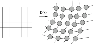
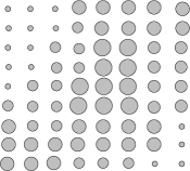
Figure 5.1. Transformation of centres of spherical balls. Space-dependent perforations.

Another example of a locally-periodic microstructure is the space-dependent perforation in concrete materials, see Fig 5.1, where a heterogeneity of the medium is given by areas of high and low diffusivity, [27]. For $\rho\in C^{1}(\mathbb{R}^{3})$, such that $0<\rho_{1}\leq\rho(x)\leq\rho_{2}<1$ for $x\in\mathbb{R}^{3}$, we consider $Y$-periodic function

$$\chi(x,y)=\begin{cases}1\quad&\text{ for }\quad|y|\leq\rho(x),\\ 0\quad&\text{ for }\quad|y|>\rho(x).\end{cases}$$

Then the characteristic function of a domain with low diffusion is given by $\chi_{\Omega^{\varepsilon}_{l}}(x)=(\mathcal{L}^{\varepsilon}_{0}\chi)(x)$. In the notation of [27], the corresponding level set function reads $S(x,y)=|y|^{2}-\rho^{2}(x)$. Showing that the locally-periodic problem provides a correct approximation for the non-periodic model and applying the locally-periodic two-scale convergence with $D(x)=I$, we should obtain the same macroscopic equations, as derived in [27] using formal asymptotic expansion. The main step of the approximation involves the following calculations. For $\varepsilon\kappa_{n}\in\Omega_{n}^{\varepsilon}$ and $k_{j}^{n}=\kappa_{n}+m_{j}$, with $j=1,\ldots I_{n}^{\varepsilon}$ and $m_{j}\in\mathbb{Z}^{3}$, considering Taylor expansion for $\rho(x)$ around $\varepsilon\kappa_{n}$, we have

$$\sum\limits_{n=1}^{N_{\varepsilon}}\int\limits_{\Omega_{n}^{\varepsilon}}\sum\limits_{j=1}^{I_{n}^{\varepsilon}}\Big{|}\chi\big{(}\varepsilon\kappa_{n},\frac{x}{\varepsilon}\big{)}-\chi\big{(}\varepsilon k_{j}^{n},\frac{x}{\varepsilon}\big{)}\Big{|}^{2}dx\leq\sum\limits_{n=1}^{N_{\varepsilon}}I_{n}^{\varepsilon}\sup\limits_{1\leq j\leq I_{n}^{\varepsilon}}\Big{\|}\chi\big{(}\varepsilon\kappa_{n},\frac{x}{\varepsilon}\big{)}-\chi\big{(}\varepsilon k_{j}^{n},\frac{x}{\varepsilon}\big{)}\Big{\|}^{2}_{L^{2}}\leq$$

$$c_{1}\sum\limits_{n=1}^{N_{\varepsilon}}I_{n}^{\varepsilon}\sup\limits_{1\leq j\leq I_{n}^{\varepsilon}}\Big{|}\big{|}\varepsilon\rho(\varepsilon\kappa_{n})\big{|}^{3}-\big{|}\varepsilon\rho(\varepsilon\kappa_{n})\pm\varepsilon\|\nabla\rho\|_{L^{\infty}}|\varepsilon m_{j}|\big{|}^{3}\Big{|}\leq c_{2}\sup\limits_{1\leq j\leq I_{n}^{\varepsilon}}|\varepsilon m_{j}|\leq c\varepsilon^{r}.$$

References

• [1] Alexandre, R. Homogenization and $\theta-2$ convergence. Proceeding of Roy. Soc. of Edinburgh, 127A (1997), pp. 441–455.
• [2] Allaire, G. Homogenization and two-scale convergence. SIAM J Math. Anal., 23 (1992), pp. 1482–1518.
• [3] Allaire, G. Shape optimization by the homogenization methods. Springer, New York, 2002.
• [4] Alt, H.W. Lineare Funktionanalysis. Springer, Berlin Heidelberg, 2002.
• [5] Baohua J., Gao, H. Mechanical properties of nanostructure of biological materials. J Mechanics Physics Solids, 52 (2004), pp 1963–1990.
• [6] Belhadj M., Cancès E., Gerbeau, J.-F., Mikelić, A. Homogenization approach to filtration through a fibrous medium. INRIA, 5277, 2004.
• [7] Belyaev, A.G., Pyatnitskii, A.L., Chechkin, G.A. Asymptotic behaviour of a solution to a boundary value problem in a perforated domain with oscillating boundary. Siberian Math. J, 39 (1998), pp 621–644.
• [8] Bourgeat, A., Mikelić, A., Wright, S. Stochastic two-scale convergence in the mean and applications J Reine Angew. Math., 456 (1994), pp 19–51.
• [9] Briane, M. Homogenénéisation de matériaux fibrés et multi-couches. PhD thesis, Université Paris VI, 1990.
• [10] Briane, M. Three models of non periodic fibrous materials obtained by homogenization. RAIRO Modél. Math.Anal.Numér., 27 (1993), pp. 759–775.
• [11] Briane, M. Homogenization of a non-periodic material. J Math. Pures Appl., 73 (1994), pp. 47–66.
• [12] Chechkin, G.A., Piatnitski, A.L. Homogenization of boundary-value problem in a locally periodic perforated domain. Applicable Analysis, 71 (1999), pp. 215–235.
• [13] Chenais, D., Mascarenhas, M. L., Trabucho, L. On the optimization of nonperiodic homogenized microstructures. RAIRO Modél. Math. Anal. Numér., 31 (1997), pp. 559–597.
• [14] Dixmier J. Von Neumann algebras. North-Holland, Amsterdam, 1981.
• [15] Fabritius, H.-O., Sachs, Ch., Triguero, P.R., Raabe, D. Influence of structural principles on the mechanics of a biological fiber-based composite material with hierarchical organization: the exoskeleton of the lobster Homorus americanus. Adv. Materials, 21 (2009), pp. 391–400.
• [16] Galdi, G. P. An introduction to the mathematical theory of the Navier-Stokes equations, I. Springer, New York, 1994.
• [17] Lemaitre, J., Chaboche, J.-L. Mechanics of solid materials. Cambridge University Press, 1990.
• [18] Lukkassen, D., Nguetseng, G., Wall, P. Two-scale convergence. Int. J Pure Appl. Math., 2 (2002), pp. 35-86.
• [19] Mascarenhas, M. L., Poliševski, D. The warping, the torsion and the Neumann problems in a quasi-periodically perforated domain. RAIRO Modél. Math. Anal. Numér., 28 (1994), pp. 37–57.
• [20] Mascarenhas, M.L., Toader, A.-M. Scale convergence in homogenization. Numer. Funct. Anal. Optimiz., 22 (2001), pp. 127–158.
• [21] Mascarenhas, M.L. Homogenization problems in locally periodic perforated domains. Asymptotic methods for elastic structures (Proc. of the International Conference, Lisbon, Portugal, 1993), 141–149, de Gruyter, Berlin, 1995.
• [22] Meier S.A. Two-scale models of reactive transport in porous media involving microstructural changes. PhD thesis, University Bremen, 2008.
• [23] Muntean, A., van Noorden, T.L. Corrector estimates for the homogenization of a locally-periodic medium with areas of low and high diffusivity. CASA-Report 11-29, 2011.
• [24] Murat, F, Tartar, L. H-convergence. in Topics in the mathematical modelling of composite materials, 21–43, Progr. Nonlinear Differential Equations Appl., 31, Birkhäuser Boston, Boston, MA, 1997.
• [25] Nguetseng G. A general convergence result for a functional related to the theory of homogenization. SIAM J Math. Anal., 20 (1989), pp. 608–623.
• [26] Nikolov, S., Petrov, M., Lymperakis, L., Friák, M., Sachs, Ch., Fabritius, H.-O., Raabe, D., Neugebauer, J. Revealing the design principles of high-performance biological composites using ab initio and multiscale simulations: the example of lobster cuticle. Adv. Mater., 21 (2009), pp. 1–8.
• [27] van Noorden, T.L., Muntean, A. Homogenization of a locally-periodic medium with areas of low and high diffusivity. European J Appl. Math., 22 (2011), pp. 493 –516.
• [28] Peskin, C.S. Fiber architecture of the left ventricular wall: an asymptotic analysis. Comm. Pure and Appl. Math., 42 (1989), pp. 79–113.
• [29] Polisevski, D. Quasi-periodic structure optimisation of the torsional rigidity. Numer. Funct. Anal. Optimiz., 15 (1994), pp 121-129.
• [30] Roy, D.M., Idorn, G.M. Concrete Microstructure. SHRP, Nat.Resear.Coun.Washington, 1993.
• [31] Schweers, E., Loffler,F. Realistic modelling of the behaviour of fibrous filters through consideration of filter structure. Powder Technol., 80 (1994) pp. 191–206.
• [32] Shkoller, S.An approximate homogenization scheme for nonperiodic materials. Comp. Math. Applic., 33 (1997), pp 15–34.
• [33] Showalter, R.E., Walkington, N.J. Micro-structure models of diffusion in fissured media. J Math. Anal. Appl., 155 (1991), pp. 1-20.