Modeling scattering polarization for probing solar magnetism

Abstract

This paper considers the problem of modeling the light polarization that emerges from an astrophysical plasma composed of atoms whose excitation state is significantly influenced by the anisotropy of the incident radiation field. In particular, it highlights how radiative transfer simulations in three-dimensional models of the “quiet” solar atmosphere may help us to probe its thermal and magnetic structure, from the near equilibrium photosphere to the highly non-equilibrium upper chromosphere. The paper finishes with predictions concerning the amplitudes and magnetic sensitivities of the linear polarization signals produced by scattering processes in two transition region lines, which should encourage us to develop UV polarimeters for sounding rockets and space telescopes with the aim of opening up a new diagnostic window in astrophysics.

1 Introduction

Consider a line of sight (LOS) that makes an angle $\theta=45^{\circ}$ with respect to the solar radius through the observed point (i.e., ${\,}{\mu}={\rm cos}\,{\theta}=0.707$) and let us make the following virtual measurements of the emergent Stokes profiles in a “non-LTE line”. Assume that the observed plasma structure is strongly magnetized (with magnetic strength $B=1200$ G), and consider two different magnetic field orientations: (1) vertical and (2) horizontal (see Fig. 1). The dotted lines of Fig. 2 show the emergent Stokes profiles produced by the Zeeman effect, which for this LOS turn out to be identical for both field orientations because of the well-known azimuth ambiguity of the Zeeman effect. However, the Stokes profiles produced by the Sun are very different. Actually, the Stokes profiles corresponding to the vertical field case are given by the solid lines of Fig. 2, while those corresponding to the horizontal field case are given by the dashed lines.

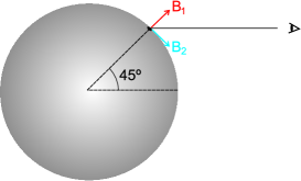
Figure 1.: The LOS and the magnetic field orientations considered in Figs. 2 and 3.

Figure 2.: Emergent Stokes profiles of the He i 10830 Å triplet for $B=1200$ G, calculated with the spectral synthesis option of the code HAZEL (from HAnle and ZEeman Light) developed by Asensio Ramos et al. (2008). The “ATOMPOL” profiles have been obtained taking into account the joint action of atomic level polarization and the Hanle and Zeeman effects, while the “NO ATOMPOL” profiles are produced by the Zeeman effect alone. The reference direction for positive Stokes $Q$ is the perpendicular to the plane formed by the solar radius vector through the observed point and the LOS.

We may thus note that

• The polarization of the Zeeman effect only depends on the orientation of the magnetic field with respect to the LOS.

• The polarization produced by the Sun depends on both the orientation of the magnetic field with respect to the LOS and on its inclination with respect to the local vertical.

Figure 3.: As in Fig. 2, but for $B=100$ G.

Why does the Sun behave this way? Because we are dealing here with an astrophysical plasma composed of atoms whose excitation state is significantly influenced by the anisotropy of the pumping radiation field. The ensuing radiative transitions produce population imbalances and quantum coherences between the magnetic sublevels pertaining to the lower and/or upper levels of the spectral line under consideration (i.e., atomic level polarization), in such a way that the populations of magnetic substates with different values of $|M|$ are different. This is termed atomic level alignment. The radiatively induced polarization of the atomic levels produces selective emission and/or selective absorption of polarization components, which give rise to linear polarization in the emergent spectral line radiation even in the absence of magnetic fields (e.g., Trujillo Bueno 2001, for a detailed review). Via the Hanle effect the atomic level polarization is sensitive to the presence of a magnetic field inclined with respect to the symmetry axis of the incident radiation field, so that it is natural to find in Fig. 2 very different results for the vertical and horizontal magnetic field cases.

What kind of Stokes profiles would we observe if the magnetic strength were much lower (say, $B=100$ G) ? As seen in Fig. 3, if $B=100$ G the circular polarization of the He i 10830 Å triplet is still dominated by the longitudinal Zeeman effect, but the linear polarization is fully controlled by atomic level polarization and the Hanle effect with no significant influence of the transverse Zeeman effect. Interestingly, this is precisely the situation we find in quiet regions of the solar atmosphere for many spectral lines, not only for the He i 10830 Å triplet considered in Figs. 2 and 3. An observational example is shown in Fig. 4, which corresponds to high-sensitivity spectropolarimetric measurements of the Ca ii IR triplet obtained in collaboration with R. Ramelli (IRSOL) using the Zürich Imaging Polarimeter (ZIMPOL) at the THEMIS telescope. This is because for weak magnetic fields (with $B{\lesssim}100$ G) the Zeeman splitting of the $\sigma$ and $\pi$ components of many spectral lines is negligible compared with the spectral line width.

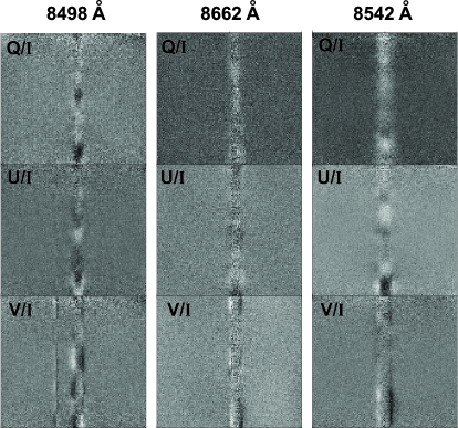
Figure 4.: An example of our recent spectropolarimetric observations of the Ca ii IR triplet in a quiet region close to the solar limb, using ZIMPOL at the telescope THEMIS of the Observatorio del Teide. Note that the sign of the $U/I$ signals fluctuates along the spatial direction of the spectrograph’s slit, which suggests spatial variations in the azimuth of the magnetic field in the quiet solar chromosphere. The reference direction for Stokes $Q$ is as in Fig. 2. From Trujillo Bueno et al. (2011).

This paper highlights how radiative transfer modeling of the scattering polarization observed in the “quiet” solar atmosphere allows us to explore its thermal and magnetic structure, but it does not provide information on numerical methods. Such information can be found in several recent reviews. For the case of partial frequency redistribution (PRD), but assuming a two-level model atom with no lower-level polarization, see Nagendra & Sampoorna (2009). For the case of realistic multilevel atoms with the possibility of atomic level polarization in all the levels, but assuming complete frequency redistribution (CRD), see Trujillo Bueno (2003). Unfortunately, a general PRD theory for modeling scattering line polarization with multilevel atoms is not yet available (e.g., Belluzzi 2011). Nevertheless, the CRD theory described in the monograph by Landi Degl’Innocenti & Landolfi (2004) is suitable for modeling the polarization observed in the Sun’s continuous radiation (see Section 2.1) and in many diagnostically important spectral lines, such as the He i 10830 Å and D₃ multiplets (e.g., Casini & Landi Degl’Innocenti 2007), the Sr i line at 4607 Å (see Sections 2.2 and 2.3), the lines of ionized cerium (Manso Sainz et al. 2006), the CN lines (e.g., Asensio Ramos & Trujillo Bueno 2003), the Li i 6708 Å line (Belluzzi et al. 2009), the Mg i $b$-lines (Trujillo Bueno 2001), the IR triplet of Ca ii (Manso Sainz & Trujillo Bueno 2003, 2010) and H_α (Štěpán & Trujillo Bueno 2010). Moreover, it can also be used for estimating the line-center scattering polarization amplitudes expected in strong resonance lines for which frequency correlations between the incoming and outgoing photons are indeed significant (e.g., the Ly_α line investigation of Section 3.1). However, PRD effects have to be taken into account in order to model the shapes of the linear polarization profiles produced by scattering in strong resonance lines (e.g., Anusha et al. 2011). Fortunately, the lower level of several resonance line transitions cannot carry atomic alignment because its total angular momentum is $J_{l}=0$ or $J_{l}=1/2$, so that PRD modeling efforts based on the standard two-level atom approach are of interest (e.g., the Mg ii k line investigation considered in Section 3.2).

2 3D modeling of scattering polarization in the quiet photosphere

This section considers some radiative transfer investigations of scattering polarization in the following three-dimensional (3D) models of the quiet solar photosphere: (1) a snapshot model taken from the hydrodynamical simulations of solar surface convection by Asplund et al. (2000) (hereafter, the HD model) and (2) a snapshot model taken from the magnetoconvection simulations with surface dynamo action carried out by Vögler & Schüssler (2007) (hereafter, the MHD model). The main aim here is to review how the modeling of observations of the intensity and linear polarization of the Sun’s continuous radiation and of the Sr i 4607 Å line allows us to probe the thermal structure and the magnetization of the quiet solar photosphere.

In both radiative transfer problems “zero-field” dichroism (see Manso Sainz & Trujillo Bueno 2003) can be neglected, so that the $4{\times}4$ propagation matrix of the Stokes-vector transfer equation is diagonal. Therefore, the relevant equation for the Stokes parameter $X$ (with $X=I,Q,U$) at a given frequency $\nu$ and direction of propagation $\vec{\Omega}$ is given by

$${{d}\over{d{\tau}}}{X}\,=\,{X}\,-\,S_{X},$$ (1)

where $d{\tau}=-{\eta_{I}}ds$ defines the monochromatic optical distance ($\tau$) along the ray, with $s$ being the corresponding geometrical distance and $\eta_{I}$ the absorption coefficient. In Eq. (1) the expressions of the source-function components are

$$S_{I}=r\,S^{*}_{I}+(1-r)B_{\nu},$$ (2)

$$S_{Q}=r\,S^{*}_{Q},$$ (3)

$$S_{U}=r\,S^{*}_{U},$$ (4)

where $r$ is a problem-dependent opacity ratio to be given below and $B_{\nu}$ the Planck function. Moreover,

$$S^{*}_{I} =\,S^{0}_{0}+w^{(2)}_{J_{u}J_{l}}\Big{\{}\frac{1}{2\sqrt{2}}(3\mu^{2}-1)S^{2}_{0}-\sqrt{3}\mu\sqrt{1-\mu^{2}}(\cos\chi{\rm Re}[{S}^{2}_{1}]-\sin\chi{\rm Im}[{S}^{2}_{1}])$$

$$\quad+\frac{\sqrt{3}}{2}(1-\mu^{2})(\cos 2\chi\,{\rm Re}[{S}^{2}_{2}]-\sin 2\chi\,{\rm Im}[{S}^{2}_{2}])\Big{\}},$$

$$S^{*}_{Q} =\,-\,w^{(2)}_{J_{u}J_{l}}\Big{\{}\frac{3}{2\sqrt{2}}(\mu^{2}-1)S^{2}_{0}-\sqrt{3}\mu\sqrt{1-\mu^{2}}(\cos\chi{\rm Re}[{S}^{2}_{1}]-\sin\chi{\rm Im}[{S}^{2}_{1}])$$

$$\quad-\frac{\sqrt{3}}{2}(1+\mu^{2})(\cos 2\chi\,{\rm Re}[{S}^{2}_{2}]-\sin 2\chi\,{\rm Im}[{S}^{2}_{2}])\Big{\}},$$

and

$$S^{*}_{U} =\,-\,w^{(2)}_{J_{u}J_{l}}\sqrt{3}\Big{\{}\sqrt{1-\mu^{2}}(\sin\chi{\rm Re}[{S}^{2}_{1}]+\cos\chi{\rm Im}[{S}^{2}_{1}])$$

$$\quad+\mu(\sin 2\chi\,{\rm Re}[{S}^{2}_{2}]+\cos 2\chi\,{\rm Im}[{S}^{2}_{2}])\Big{\}},$$

where $\theta={\rm arccos}\,({\mu})$ and $\chi$ are the inclination with respect to the solar local vertical and azimuth of the ray, respectively, $w^{(2)}_{J_{u}J_{\ell}}$ is a coefficient that is equal to unity for the problems considered in the following subsections, and the equations that govern the quantities $S^{0}_{0}$, $S^{2}_{0}$, ${\rm Re}[{S}^{2}_{1}]$, ${\rm Im}[{S}^{2}_{1}]$, ${\rm Re}[{S}^{2}_{2}]$ and ${\rm Im}[{S}^{2}_{2}]$ will be given below for each particular problem considered. We point out that in these equations the reference direction for Stokes $Q$ is the perpendicular to the plane formed by the ray’s propagation direction and the vertical Z-axis.

2.1 Polarization of the Sun’s continuous spectrum

The dominant contribution to the linear polarization of the visible continuous spectrum comes from Rayleigh scattering by neutral hydrogen in its ground state (Lyman scattering) and Thomson scattering by free electrons (Chandrasekhar 1960). The contribution of these processes to the total absorption coefficient ($\eta_{I}$) is quantified by ${\sigma}_{c}\,=\,{\sigma}_{T}\,N_{e}+\,{\sigma}_{R}\,n_{1}(H)$, where $\sigma_{T}=6.653{\times}10^{-25}\,{\rm cm}^{2}$ is the Thomson scattering cross section, $N_{e}$ the electron number density, $n_{1}(H)$ the population of the ground level of hydrogen, and $\sigma_{R}$ the wavelength-dependent Rayleigh cross section. The continuum absorption coefficient is given by ${\eta_{I}}\,=\kappa_{c}\,+\,{\sigma}_{c}$, where $\kappa_{c}$ contains all the relevant non-scattering contributions (e.g., the bound-free transitions in the H^- ion). The expressions of the $S_{X}$ source function components can be found easily by taking $r={{\sigma_{c}}\over{\kappa_{c}+\sigma_{c}}}$ and ${S^{0}_{0}}={J}^{0}_{0}$, ${S^{2}_{0}}={J}^{2}_{0}$, ${{\rm Re}[{S}^{2}_{1}]}={\rm Re}[{J}^{2}_{1}]$, ${{\rm Im}[{S}^{2}_{1}}]=-{\rm Im}[{J}{}^{2}_{1}]$, ${{\rm Re}[{S}^{2}_{2}]}={\rm Re}[{J}{}^{2}_{2}]$ and ${{\rm Im}[{S}^{2}_{2}}]=-{\rm Im}[{J}{}^{2}_{2}]$ in Eqs. (5)-(7) (e.g., Trujillo Bueno & Shchukina 2009).

Note that the ${{J}}^{K}_{Q}$ quantities (with $K=0,2$ and $Q=0,1,2$) are the spherical components of the radiation field tensor (see § 5.11 in Landi Degl’Innocenti & Landolfi 2004), which quantify the symmetry properties of the radiation field at the spatial point under consideration. Thus, ${J}{}^{0}_{0}$ is the familiar mean intensity, ${J}^{2}_{0}{\approx}\oint\frac{{\rm d}\vec{\Omega}}{4\pi}\frac{1}{2\sqrt{2}}(3\mu^{2}-1){{I_{\nu,\vec{\Omega}}}}\,$ quantifies its anisotropy, while the real and imaginary parts of ${{J}}^{2}_{Q}$ (with $Q=1,2$) (i.e., ${\rm Re}[{J}{}^{2}_{Q}]$ and ${\rm Im}[{J}{}^{2}_{Q}]$, respectively) measure the breaking of the axial symmetry. Obviously, the real and imaginary parts of ${J}{}^{2}_{1}$ and ${J}{}^{2}_{2}$ are zero in a plane-parallel or spherically symmetric model atmosphere, but they can have significant positive and negative values in a 3D stellar atmospheric model (see figure 3 of Trujillo Bueno & Shchukina 2009). Therefore, Eqs. (6) and (7) tell us that $U=0$ in 1D models, and that the key observational signatures of the symmetry breaking effects in a 3D model (caused by its horizontal atmospheric inhomogeneities) are non-zero $U$ signals at any on-disk position and non-zero Stokes $Q$ and $U$ signals for the LOS with $\mu=1$, which corresponds to forward-scattering geometry.

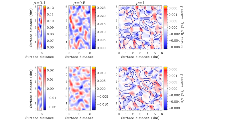
Figure 5.: The continuum scattering polarization signals at 4600 Å calculated for three line of sights in Asplund et al.’s (2000) hydrodynamical model of the solar photosphere (i.e., the HD model), accounting for the diffraction limit effect of a 1-m telescope. Although the polarization amplitudes are very low at 4600 Å, they are one order of magnitude larger at 3000 Å. The solid line contours in the right panels delineate the upflowing granular regions. From Trujillo Bueno & Shchukina (2009).

Figure 5 shows the $Q/I$ and $U/I$ images that we would see at 4600 Å if we could observe with high polarimetric precision the solar continuum polarization at very high spatial and temporal resolution. Obviously, without spatial and/or temporal resolution $U/I{\approx}0$ and the only observable quantity would be $Q/I$, whose wavelength variation at a solar disk position close to the limb has been determined semi-empirically by Stenflo (2005). Note that the spatially-averaged $Q/I$ of the solar continuum radiation at each $\mu$ position is largely determined by the effective polarizability, $r={{\sigma_{c}}/({\kappa_{c}+\sigma_{c}}})$, and by the fractional radiation field’s anisotropy, $J^{2}_{0}/J^{0}_{0}$, which in turn depend on the density and thermal structure of the stellar atmosphere under consideration. Therefore, the more realistic the thermal and density structure of a given solar atmospheric model is, the closer to the empirical data will be the calculated linear polarization of the solar continuum radiation. Interestingly, Fig. 12 of Trujillo Bueno & Shchukina (2009) demonstrates that 3D radiative transfer modeling of the polarization of the Sun’s continuous spectrum in the above-mentioned 3D hydrodynamical model of the solar photosphere shows a notable agreement with Stenflo’s (2005) semi-empirical data, significantly better than that obtained via the use of 1D semi-empirical models.

2.2 The polarization of the Sr i 4607 Å line and the Hanle effect of a microturbulent field in a 3D hydrodynamical model of the quiet photosphere

In this and in the following subsection we focus on the diagnostic problem of the magnetism of the quiet solar photosphere (e.g., the review by Sánchez Almeida 2004). To this end, we need to measure and interpret polarization in spectral lines. It is important to note that determining the mean magnetization of the quiet Sun requires finding how much flux resides at small scales and that, to this end, it is crucial to measure and interpret the linear polarization produced by atomic level polarization and its modification by the Hanle effect.

If at the spatial grid point under consideration the magnetic field of strength $B$ is assumed to have an isotropic distribution of orientations within a volume ${\cal L}^{3}$, with ${\cal L}$ the mean-free-path of the line photons, the equations that govern the $S^{K}_{Q}$ quantities of Eqs. (5)-(7) are (Trujillo Bueno & Manso Sainz 1999):

$$S^{0}_{0}\,=\,(1-\epsilon){{\bar{J}}}_{0}^{0}\,+\,{\epsilon}\,B_{\nu},$$ (8)

and

$$\left(\begin{array}[]{l}{S^{2}_{0}}\\ \\ {{\rm Re}[{S}^{2}_{1}}]\\ \\ {{\rm Im}[{S}^{2}_{1}}]\\ \\ {{\rm Re}[{S}^{2}_{2}}]\\ \\ {{\rm Im}[{S}^{2}_{2}}]\end{array}\right)=w^{(2)}_{J_{u}J_{l}}\,{{(1-\epsilon)}\over{1+{\delta}^{(2)}(1-\epsilon)}}\,\left(\begin{array}[]{r}{{\bar{J}}}^{2}_{0}\\ \\ {\rm Re}[{{\bar{J}}}{}^{2}_{1}]\\ \\ -{\rm Im}[{{\bar{J}}}{}^{2}_{1}]\\ \\ {\rm Re}[{{\bar{J}}}{}^{2}_{2}]\\ \\ -{\rm Im}[{{\bar{J}}}{}^{2}_{2}]\end{array}\right)\,{\cal{H}}^{(2)}\,,$$ (27)

where $\epsilon$ can be interpreted as the probability that an atomic excitation event is due to inelastic collisions with electrons, $\delta^{(2)}$ is the upper-level depolarizing rate (in units of the Einstein $A_{ul}$ coefficient) due to elastic collisions with neutral hydrogen atoms, and ${\cal{H}}^{(2)}$ is the Hanle depolarization factor whose value is ${\cal{H}}^{(2)}=1$ for $B=0$ G and ${\cal{H}}^{(2)}=1/5$ for $B>B_{\rm satur}$ (where $B_{\rm satur}$ is the Hanle saturation field, which is at least 200 G for the Sr i 4607 Å line). It is important to note that for the spectral line cases considered here and in the following sections the radiation field tensors are given by angular and frequency-weighted averages of the Stokes parameters, with the Voigt profile $\phi_{\nu}$ as the frequency-dependent weighting function. For this reason, in Eqs. (8) and (9) they are instead denoted with the symbol $\bar{J}^{K}_{Q}$. It is also worthwhile pointing out that for the spectral line case ${S_{Q}^{K}}\,=\,{\frac{2h{\nu}^{3}}{c^{2}}}{\frac{2{J}_{l}+1}{\sqrt{2{J}_{u}+1}}}{\rho}_{Q}^{K}$, with ${\rho}^{K}_{Q}$ being the multipolar components of the upper-level density matrix normalized to the overall population of the transition’s lower level. Therefore, Eq. (9) describes the transfer to the atomic system of the symmetry properties of the radiation field, and note that it is the largest for line transitions with $w^{(2)}_{J_{u}J_{l}}=1$ and when in the absence of magnetic and collisional depolarization. For the Sr i 4607 Å line $J_{l}=0$, $J_{u}=1$ and $w^{(2)}_{10}=1$. Moreover, in Eqs. (2)-(4) we have now $r=\kappa_{l}\phi_{\nu}/(\kappa_{l}\phi_{\nu}+\kappa_{c})$, with $\kappa_{l}$ the line-integrated opacity.

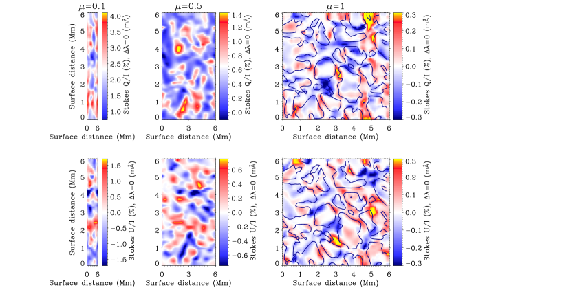
Figure 6.: The fractional linear polarization amplitudes of the Sr i 4607 Å line calculated in the HD model of the solar photosphere, neglecting any interaction with the continuum polarization because at ${\lambda}4607$ it is almost two orders of magnitude smaller, as shown in Fig. 5. From Trujillo Bueno & Shchukina (2007).

Figure 6 shows the center-to-limb variation of the $Q/I$ and $U/I$ line-center signals of the Sr i 4607 Å line, which we have obtained by solving the scattering line polarization problem in the above-mentioned HD model, without including any magnetic field, but accounting for the diffraction limit effect of a 1m telescope. Note that the calculated linear polarization amplitudes have sizable values and fluctuations, even at the very center of the solar disk, where we observe the forward scattering case (e.g., the standard deviations of the $Q/I$ and $U/I$ fluctuations are approximately $0.3\%$ at $\mu=0.5$). Trujillo Bueno & Shchukina (2007) pointed out that the predicted small-scale patterns in $Q/I$ and $U/I$ are of great diagnostic value, because they are sensitive to the thermal, dynamic and magnetic structure of the quiet solar atmosphere. Therefore, it would be important to try to observe them with an imaging polarimeter attached to a suitable telescope, such as that of the SUNRISE balloon-borne telescope.

For the moment, the scattering polarization observations of the Sr i 4607 Å line that have been published lack spatial resolution (e.g., see the data points of Fig. 7). Interestingly, when the calculated $I$, $Q$ and $U$ profiles at each $\mu$ solar-disk position are spatially averaged over scales larger than those of the solar granulation pattern we obtain $U/I{\approx}0$ and the $Q/I$ vs. $\mu$ line-center amplitudes given by the green dotted line of Fig. 7. The very significant discrepancy between the observed and the calculated scattering polarization signals led Trujillo Bueno et al. (2004) to the following conclusion: the internetwork regions of the quiet solar photosphere are permeated by a spatially unresolved tangled magnetic field, whose mean field strength at heights $h{\approx}300$ km above the visible solar surface is ${\langle B\rangle}{\approx}130$ G when no distinction is made between granular and intergranular regions. This first conclusion was reached by modeling the observed scattering line polarization through the self-consistent solution of Eqs. (8), (9) and (1) in the above-mentioned hydrodynamical model. Note that such a 3D photospheric model is unmagnetized and that, therefore, our ${\langle B\rangle}{\approx}130$ G conclusion is based on the following approximations for the description of the quiet Sun magnetic field that produces Hanle depolarization: (1) that the magnetic field is tangled at subresolution scales, with an isotropic distribution of directions and (2) that the shape of the probability distribution function, describing the fraction of quiet Sun occupied by magnetic fields of strength $B$, is exponential (i.e., ${\rm PDF}(B)={1\over{{\langle B\rangle}}}{{\rm e}^{-B/{\langle B\rangle}}}$).

2.3 The polarization of the Sr i 4607 Å line and the Hanle effect in a 3D magneto-convection model of the quiet photosphere with surface dynamo action

If at the spatial grid point under consideration the magnetic field has a given strength $B$, inclination $\theta_{B}$ and azimuth $\chi_{B}$ (e.g., as is the case with the magnetic field of magnetoconvection simulations) the equations that govern the $S^{K}_{Q}$ quantities of Eq. (5)-(7) are (Manso Sainz & Trujillo Bueno 1999):

$$S^{0}_{0}\,=\,(1-\epsilon){\bar{J}}_{0}^{0}\,+\,{\epsilon}\,B_{\nu},$$ (28)

$$\left(\begin{array}[]{l}{S^{2}_{0}}\\ \\ {{\rm Re}[{S}^{2}_{1}}]\\ \\ {{\rm Im}[{S}^{2}_{1}}]\\ \\ {{\rm Re}[{S}^{2}_{2}}]\\ \\ {{\rm Im}[{S}^{2}_{2}}]\end{array}\right)=w^{(2)}_{J_{u}J_{l}}\,{{(1-\epsilon)}\over{1+{\delta}^{(2)}(1-\epsilon)}}\left(\begin{array}[]{r}{\bar{J}}^{2}_{0}\\ \\ {\rm Re}[{J}{}^{2}_{1}]\\ \\ -{\rm Im}[{J}{}^{2}_{1}]\\ \\ {\rm Re}[{J}{}^{2}_{2}]\\ \\ -{\rm Im}[{J}{}^{2}_{2}]\end{array}\right)\,$$ (47)

$$\hskip 72.26999pt-{\Gamma_{u}}\,{{(1-\epsilon)}\over{1+{\delta}^{(2)}(1-\epsilon)}}\,\left(\begin{array}[]{cccccc}0&M_{12}&M_{13}&0&0\\ \\ M_{21}&0&M_{23}&M_{24}&M_{25}\\ \\ M_{31}&M_{32}&0&M_{34}&M_{35}\\ \\ 0&M_{42}&M_{43}&0&M_{45}\\ \\ 0&M_{52}&M_{53}&M_{54}&0\end{array}\right)\left(\begin{array}[]{l}{S^{2}_{0}}\\ \\ {{\rm Re}[{S}^{2}_{1}}]\\ \\ {{\rm Im}[{S}^{2}_{1}}]\\ \\ {{\rm Re}[{S}^{2}_{2}}]\\ \\ {{\rm Im}[{S}^{2}_{2}}]\end{array}\right)\,,$$ (66)

where ${\Gamma_{u}}=8.79\times 10^{6}g_{u}B/A_{ul}$ (with $g_{u}$ as the upper-level Landé factor, $B$ as the magnetic strength in gauss and $A_{ul}$ as the Einstein coefficient for spontaneous emission in ${\rm s}^{-1}$). The $M_{ij}$-coefficients of the magnetic kernel ${\bf M}$ depend on the inclination ($\theta_{B}$) of the local magnetic field vector with respect to the vertical Z-axis and on its azimuth ($\chi_{B}$). These equations for the ${S_{Q}^{K}}$ multipolar components have a clear physical meaning. In particular, note that the magnetic operator ${\bf M}$ couples locally the $K=2$ components among them (the Hanle effect).

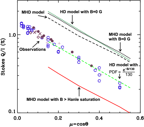
Figure 7.: Center-to-limb variation of the (spatially-averaged) $Q/I$ scattering amplitudes of the photospheric line of Sr i at 4607 Å. The data correspond to various observations taken by several authors during a minimum and a maximum of the solar activity cycle. The two green lines show scattering polarization amplitudes calculated in the 3D hydrodynamical model of Asplund et al. (2000), without including any magnetic field (green dotted line) and including the Hanle depolarization of a microturbulent field with an exponential PDF characterized by a mean field strength $\langle B\rangle{=}130$ G (green dashed line). The two black lines show scattering polarization amplitudes calculated in the MHD model of Vögler & Schüssler (2007), neglecting its magnetic field (black dotted line) and taking into account the Hanle depolarization of its magnetic field (black dashed line). We point out that the observations can be approximately fitted by multiplying each grid-point magnetic strength by a scaling factor, such that at heights $h{\approx}300$ km the resulting $\langle B\rangle$ is approximately 130 G. The red solid line shows the calculated scattering polarization amplitudes when imposing $B>B_{\rm satur}$ at each grid point in the MHD model. For more information see Shchukina & Trujillo Bueno (2011).

The black dotted line of Fig. 7 shows the spatially averaged scattering polarization amplitudes of the Sr i 4607 Å line calculated by Shchukina & Trujillo Bueno (2011) in the MHD model of Vögler & Schüssler (2007), but after imposing $B=0$ G at each spatial grid point. Interestingly, the resulting scattering polarization amplitudes are similar (but not identical) to those computed in the HD model (see the green dotted line). The differences between the two curves are due to the fact that the thermal and density structure of the two snapshot models are not fully identical. The black dashed line shows the $Q/I$ amplitudes that Shchukina & Trujillo Bueno (2011) obtain when taking into account the Hanle depolarization produced by the actual magnetic field of the MHD surface dynamo model, whose magnetic Reynolds number is $R_{m}{\approx}2600$. The fact that the resulting Hanle depolarization is too small to explain the observations is not surprising because the mean field strength at a height of about 300 km in the MHD snapshot model is only $\langle B\rangle\,{\approx}15$ G (i.e., about an order of magnitude smaller than the $\langle B\rangle\,{\approx}130$ G value inferred by Trujillo Bueno et al. (2004)). In order to investigate whether we can fit the observations of Fig. 7 with a magnetic field topology identical to that of the MHD surface dynamo snapshot we have increased only the magnetic strength of each spatial grid point by multiplying it by a scaling factor. Remarkably, the mean field strength that we have to reach this way to fit the observations of Fig. 7 is about 130 G (see Shchukina & Trujillo Bueno 2011). Note that this conclusion has now been reached without assuming that the shape of the PDF is exponential and without using the microturbulent field approximation. Clearly, both approximations were suitable to find the mean field strength of the “hidden” field (Trujillo Bueno et al. 2004). In particular, it is interesting to note that the fact that the red line of Fig. 7 practically coincides with 1/5 of the zero-field linear polarization amplitudes indicates that the microturbulent field approximation is indeed a suitable one.

Finally, it may be of interest to mention the second conclusion of Trujillo Bueno et al. (2004), which resulted from their joint analysis of the Hanle effect in the Sr i 4607 Å line and in C₂ lines of the Swan system (see also Trujillo Bueno et al. 2006): the downward-moving intergranular lane plasma is pervaded by relatively strong tangled fields at subresolution scales, with $\langle B\rangle\,{>}B_{\rm satur}$ (where $B_{\rm satur}\,{\approx}\,200$ G is a lower limit to the Hanle saturation field of the Sr i 4607 Å line). This conclusion, which implies that most of the flux and magnetic energy reside on still unresolved scales, is also supported by the recent investigation of Shchukina & Trujillo Bueno (2011).

3 Scattering polarization and the Hanle effect in transition region lines

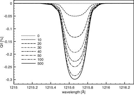
Figure 8.: Theoretical estimate of the fractional linear polarization signals of the Ly_α line produced by forward scattering processes in the solar transition region, taking into account the Hanle effect caused by the presence of a horizontal magnetic field with the indicated strength (in G). The reference direction for positive Stokes $Q$ is the parallel to the magnetic field vector. Note how in forward scattering geometry (i.e., for a LOS with $\mu=1$) the fractional linear polarization amplitude of Ly_α increases as the magnetic strength of the inclined field is increased. The semi-empirical model used for the radiative transfer calculations is FAL-C (see Fontenla et al. 1993). From Trujillo Bueno et al. (2011).

A recent review on spectropolarimetric investigations of the magnetization of the quiet Sun chromosphere can be found in Trujillo Bueno (2010). In the remaining part of this section I focus instead on advancing some results of two recent theoretical investigations about the linear polarization signals expected for the hydrogen Ly_α line at 1215 Å and the Mg ii k-line at 2795 Å, produced by scattering processes in the solar transition region plasma itself.

3.1 Ly_α in the solar transition region

The intensity profile of the hydrogen Ly_α line has been measured on the solar disk by several instruments on board rockets or space-based telescopes (e.g., by the SUMER spectrometer on SOHO). These measurements show that Ly_α is always in emission at all on-disk positions and times, and that the emission originates in the upper chromosphere and transition region. The center-to-limb variation of the observed Ly_α intensity profiles in the quiet Sun is very small or negligible (e.g., Curdt et al. 2008). This implies that the outgoing radiation shows no significant variation with the heliocentric angle $\theta$. However, this does not mean that the illumination of the transition region atoms is isotropic – which would imply that scattering polarization in Ly_α is zero. The incoming radiation (i.e., the one which illuminates the transition region atoms from “above”) calculated by J. Štěpán (IAC) and I in semi-empirical models of the solar atmosphere shows significant limb brightening, so that atoms in the transition region are indeed irradiated by an anisotropic radiation field. The ensuing radiation pumping induces population imbalances among the sublevels of the upper level $2p^{2}{\rm P}_{3/2}$ of the Ly_α line, which is the only hydrogen level that makes a significant contribution to its scattering polarization. The atomic polarization of the $2p^{2}{\rm P}_{3/2}$ level produces linear polarization in Ly_α, which is modified by the presence of a magnetic field through the Hanle effect. The $Q/I$ amplitudes we have calculated in various models of the solar atmosphere vary between 0.5% and 0.05%, approximately, depending on the strength of the magnetic field and the LOS. For example, Fig. 8 shows the calculated linear polarization signals caused by the Hanle effect in the forward-scattering geometry of a disk-center observation. Note that in order to be able to detect the presence of a horizontal magnetic field of 30 G in the bulk of the solar transition region the polarimetric sensitivity of the measurement should be at least 0.1%. Interestingly, this Ly_α investigation (see also Trujillo Bueno et al. 2005) has motivated a proposal to NASA (led by Japan, USA and Spain) for the development of a Chromospheric Lyman-Alpha Spectro-Polarimeter (CLASP) for a sounding rocket (see Ishikawa et al. 2011).

3.2 Mg ii k in the solar transition region

The CRD theory on which the radiative transfer modeling of the previous sections is based treats the scattering line polarization phenomenon as the temporal succession of 1st-order absorption and re-emission processes, interpreted as statistically independent events. As mentioned in the introduction, this theory can also be used for estimating the expected scattering polarization amplitudes in strong resonance lines for which frequency correlations between the incoming and outgoing photons are indeed significant (e.g., see Fig. 8 for the case of Ly_α in forward scattering geometry). However, it is important to emphasize that PRD effects have to be taken into account in order to be able to provide reliable predictions on the shapes of the linear polarization profiles produced by scattering in strong resonance lines like Ly_α and Mg ii k. Recently, Sampoorna et al. (2010) have studied in great detail the sensitivity of PRD scattering polarization profiles to various atmospheric parameters. To this end, the authors applied the very efficient radiative transfer method described in Sampoorna & Trujillo Bueno (2010). An example of the type of investigations that can be carried out with a PRD radiative transfer code based on that numerical method is considered in Fig. 9, which shows the complicated shape of the $Q/I$ profile of the Mg ii k-line caused by scattering processes with PRD effects in a semi-empirical model of the solar chromosphere and transition region.

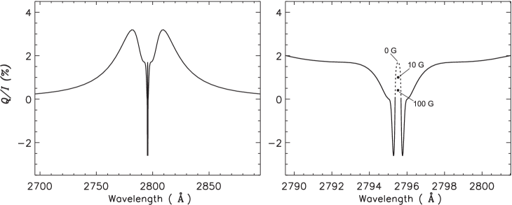
Figure 9.: The close to the limb ($\mu=0.1$) $Q/I$ profile of the Mg ii k-line produced by line scattering processes in the FAL-C semi-empirical model of the solar atmosphere, taking into account PRD effects as explained in Sampoorna & Trujillo Bueno (2010) and without accounting for the continuum polarization contribution. The right panel shows better the line-core spectral region, indicating the line-center Hanle depolarization produced by a random-azimuth horizontal magnetic field with the indicated strength. The dotted-line shows the only part of the PRD $Q/I$ profile that can be estimated via the CRD theory. The reference direction for Stokes $Q$ is as in Fig. 2. This figure stems from a collaboration between M. Sampoorna (IIA), J. Štěpán (IAC) and J. Trujillo Bueno (IAC).

Off-limb observations of spicules in Ly_α and Mg ii k at various heights above the visible solar limb are expected to show higher polarization amplitudes. Both types of observations (on-disk and off-limb) would provide precious information on the physical conditions of the solar transition region from the chromosphere to the $10^{6}$ K solar coronal plasma, even with a spatial resolution of only 1 or 2 arcseconds.

4 Concluding comment

Radiative transfer modeling of solar light polarization is the essential link between theory and observations. In general, realistic modeling requires solving a very complicated and still unsolved problem: non-LTE, multilevel, PRD radiative transfer, taking into account the joint action of the Hanle and Zeeman effects in 3D atmospheric models of the extended solar atmosphere. Fortunately, the Sun is subtle but not malicious: it allows us to learn how it works in a stepwise manner, while continuously motivating us to open up new research windows in astrophysics through the development of increasingly novel theories, instruments, modeling and data analysis techniques.

Acknowledgments

The results discussed here owe much to collaborations with N. Shchukina, J. Štěpán, M. Sampoorna, R. Ramelli, R. Manso Sainz, M. Bianda and A. Asensio Ramos, and I thank them for fruitful discussions. I am also grateful to L. Belluzzi for carefully reviewing the paper. Finantial support by the Spanish Ministry of Science through projects AYA2010-18029 (Solar Magnetism and Astrophysical Spectropolarimetry) and CONSOLIDER INGENIO CSD2009-00038 (Molecular Astrophysics: The Herschel and Alma Era) is gratefully acknowledged.

References

- Anusha et al. (2011) Anusha, L. S. et al. 2011, these proceedings
- Asensio Ramos & Trujillo Bueno (2003) Asensio Ramos, A., & Trujillo Bueno, J. 2003, in Solar Polarization 3, eds. J. Trujillo Bueno & J. Sánchez Almeida, ASP Conf. Ser. Vol. 307, 195
- Asensio Ramos et al. (2008) Asensio Ramos, A., Trujillo Bueno, J., & Landi Degl’Innocenti, E. 2008, ApJ, 683, 542
- Asplund et al. (2000) Asplund, M., Nordlund, Å., Trampedach, R., Allende-Prieto, C., & Stein, R.F. 2000, A&A, 359, 729
- Belluzzi (2011) Belluzzi, L. 2011, these proceedings
- Belluzzi et al. (2009) Belluzzi, L., Landi Degl’Innocenti, E., & Trujillo Bueno, J. 2009, ApJ, 705, 218
- Casini & Landi Degl’Innocenti (2007) Casini, R., & Landi Degl’Innocenti, E. 2007, in Plasma Polarization Spectroscopy, eds. T. Fujimoto & A. Iwamae (Berlin: Springer), 247
- Cattaneo (1999) Cattaneo, F. 1999, ApJ, 515, L39
- Chandrasekhar (1960) Chandrasekhar, S. 1960, Radiative Transfer, Dover Publications, Inc.
- Curdt et al. (2008) Curdt, W., Tian, H., Teriaca, L., Schühle, U., & Lemaire, P. 2008, A&A, 492, L9
- Faurobert-Scholl et al. (1995) Faurobert-Scholl, M., Feautrier, N., Machefert, F., Petrovay, K., & Spielfiedel, A. 1995, A&A, 298, 289
- Fontenla et al. (1993) Fontenla, J. M., Avrett, E. H., & Loeser, R. 1993, ApJ, 406, 319
- Ishikawa et al. (2011) Ishikawa, R. et al. 2011, these proceedings
- Landi Degl’Innocenti & Landolfi (2004) Landi Degl’Innocenti, E., & Landolfi, M. 2004, Polarization in Spectral Lines, (Dordrecht: Kluwer)
- Manso Sainz & Trujillo Bueno (1999) Manso Sainz, R., & Trujillo Bueno, J. 1999, in Solar Polarization, eds. K. N. Nagendra & J. O. Stenflo, ASSL 243 (Dordrecht: Kluwer), 143
- Manso Sainz & Trujillo Bueno (2003) Manso Sainz, R., & Trujillo Bueno, J. 2003, Phys.Rev.Lett, 91, 111102
- Manso Sainz & Trujillo Bueno (2010) Manso Sainz, R., & Trujillo Bueno, J. 2010, ApJ, 722, 1416
- Manso Sainz et al. (2006) Manso Sainz, R., Landi Degl’Innocenti, E., & Trujillo Bueno, J. 2006, A&A, 447, 1125
- Nagendra & Sampoorna (2009) Nagendra, K. N., & Sampoorna, M. 2009, in Solar Polarization 5, eds. S. Berdyugina, K. N. Nagendra, & R. Ramelli, ASP Conf. Ser. Vol. 405, 261
- Sampoorna & Trujillo Bueno (2010) Sampoorna, M., & Trujillo Bueno, J. 2010, ApJ, 712, 1331
- Sampoorna et al. (2010) Sampoorna, M., Trujillo Bueno, J., & Landi Degl’Innocenti, E. 2010, ApJ, 722, 1269
- Sánchez Almeida (2004) Sánchez Almeida, J. 2004, in The Solar-B Mission and the Forefront of Solar Physics, eds. T. Sakurai & T. Sekii, ASP Conf. Ser. Vol. 325, 115
- Shchukina & Trujillo Bueno (2011) Shchukina, N. & Trujillo Bueno, J. 2011, ApJ, 731, L21
- Stenflo (1982) Stenflo, J. O. 1982, Solar Phys., 80, 209
- Stenflo (2005) Stenflo, J. O. 2005, A&A, 429, 713
- Štěpán & Trujillo Bueno (2010) Štěpán, J., & Trujillo Bueno, J. 2010, ApJ, 711, L133
- Thelen & Cattaneo (2000) Thelen, J. C., & Cattaneo, F. 2000, MNRAS, 315, L13
- Trujillo Bueno (2001) Trujillo Bueno, J. 2001, in Advanced Solar Polarimetry: Theory, Observation, and Instrumentation, ed. M. Sigwarth, ASP Conf. Ser. Vol. 236, 161
- Trujillo Bueno (2003) Trujillo Bueno, J. 2003, in Stellar Atmosphere Modeling, eds. I. Hubeny, D. Mihalas & K. Werner, ASP Conf. Ser. Vol. 288, 551
- Trujillo Bueno (2010) Trujillo Bueno, J. 2010, in Chromospheric Structure and Dynamics; eds. A. Tritschler, K. Reardon & H. Uitenbroek, Mem. Soc. Astr. Ital., (arXiv:1002.2615)
- Trujillo Bueno & Manso Sainz (1999) Trujillo Bueno, J., & Manso Sainz, R. 1999, ApJ, 516, 436
- Trujillo Bueno & Shchukina (2007) Trujillo Bueno, J., & Shchukina, N. 2007, ApJ, 664, L135
- Trujillo Bueno & Shchukina (2009) Trujillo Bueno, J., & Shchukina, N. 2009, ApJ, 694, 1364
- Trujillo Bueno et al. (2006) Trujillo Bueno, J., Asensio Ramos, A., & Shchukina, N. 2006, in Solar Polarization 4, eds. R. Casini & B. W. Lites, ASP Conf. Ser. Vol. 358, 269
- Trujillo Bueno et al. (2004) Trujillo Bueno, J., Shchukina, N., & Asensio Ramos, A. 2004, Nat, 430, 326
- Trujillo Bueno et al. (2011) Trujillo Bueno, J., Štěpán, J., et al. 2011, in preparation.
- Trujillo Bueno et al. (2011) Trujillo Bueno, J., Ramelli, R., Manso Sainz, R., & Bianda, M. 2011, in preparation.
- Trujillo Bueno et al. (2005) Trujillo Bueno, J., Landi Degl’Innocenti, E., Casini, R., & Martínez Pillet, V. 2005, in Trends in Space Science and Cosmic Vision 2020, eds. F. Favata, J. Sanz-Forcada & A. Giménez, ESA SP-588, 203
- Vögler & Schüssler (2007) Vögler, A., & Schüssler, M. 2007, A&A, 465, L43