Static properties of condensates Boson systems Dynamic properties of condensates

Tonks-Girardeau gas, super-Tonks-Girardeau gas, and bound states of one-dimensional bosons in a hard-wall trap

Abstract

We investigate the Bose gas with repulsive or attractive interactions between atoms in the scheme of Bethe Ansatz equation in a hard wall trap. Three typical quantum phases in the current research of 1D interacting cold atoms are clarified in terms of the energy spectrum, single particle density distribution and two-particle correlation function. We identify two matching points in the phase diagram, i.e. the TG and STG gas show the same profiles at the strongly interacting point $-1/\gamma=0$, and in the weakly interacting limit $\gamma=0$ the ground states TG and BS join to each other smoothly.

Recently experiments and theories have made a great progress in one dimensional quantum gases [1]. Thanks to the Feshbach resonance as well as the confinement-induced resonance (CIR) [2, 3, 4], the interaction strength between atoms can be tuned exactly. The first breakthrough in experiment is the realization of Tonks-Girardeau (TG) gases [5, 6] of bosons with strongly repulsive interaction. The atoms in TG gas stay in ground state and the wave function and energy was found by Girardeau in 1960 using a Fermi-Bose (FB) mapping [7], leading to fermionization of many properties of this Bose system. The many-body properties were determined explicitly for a bosonic Tonks-Girardeau gas confined in the potential of a harmonic trap [8, 9] or a hard wall trap [10] with a tunable $\delta$-function barrier at the trap center and related work has been done for Bose-Ferimi mixture [11, 9] and finite interacting strength [12, 13, 14].

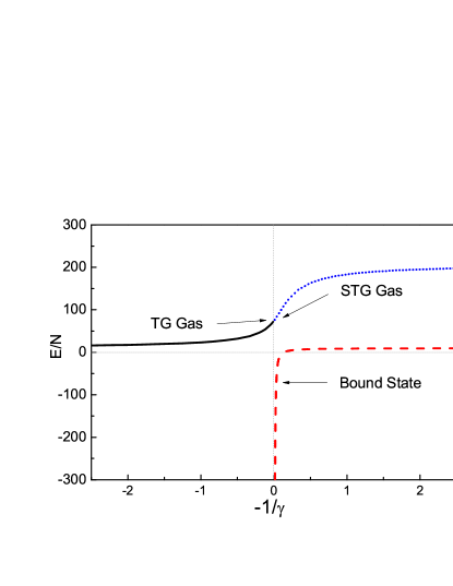
Figure 1: (Color online) The energy spectrum of $N=4$ bosons for the ground states and one of the excited states in the full interacting regime. Quantum phases of TG, STG and Bound State are clearly classified into three branches solution of Bethe Ansatz Equations.

The second important experiment is the realization of the super Tonks-Girardeau (STG) gas [15], where the Cesium atoms are prepared in a long-lived, strongly interacting, excited state. Unlike the strong repulsively interacting TG gas, the interaction of bosons in STG state is attractive. Although the TG gas has proved very successful both in theories and experiments, bosons with attractive interaction start to attract more and more attention only recently. In fact, if the interaction is finite and negative, the ground state is McGuire’s cluster state [16, 17], which is a bound state and would decay quickly via molecular channels. In the original proposal, the STG gas-like state corresponds to a highly excited Bethe state in the integrable interacting Bose gas for which the bosons acquire hard-core behavior [19, 18]. Experimentally the STG gas was realized through a sudden quench of the interaction parameter [20]. On the other hand, the ground state of a strongly attractive spin-1/2 Fermi gas can be effectively described by the STG gas [21].

Exact solutions are available only in very few limiting cases. 1D Bose gas with arbitrary repulsive interaction strength was solved by Lieb and Liniger [22] using the Bethe ansatz method in which particles are constrained by periodic boundary conditions on a line of length $L$. As far as the trapping of the atoms is concerned, a solution was given for two $\delta$-interacting particles in a harmonic trap in [23] and the STG wave function for $N=2$ particles is found to be identical to the hard-sphere bose gas [24] given exactly in terms of a parabolic cylinder function. It is very interesting to consider what happens to the above mentioned three branch solutions of 1D Bose gas when the atoms are confined in a hard wall trap, i.e., under the open boundary condition. Interacting bosons in a hard-wall trap is one of the few integrable examples of interacting many-body models and its exact solution has been obtained with the superposition of Bethe’s wave function for the repulsive interaction in a seminal paper by [25]. For a finite number of bosons and finite system size, boundary effects are expected to be pronounced at low temperature. Indeed, significantly different quantum effects should be exhibited by a finite number of bosons confined in a finite hard wall box.

Here we study the property of a few bosons trapped in 1D hard wall trap by numerically solving the Bethe Ansatz equations in the full interacting regime. We compare the energy of the system, the one body density matrix and the two-particle correlation function both in the ground state for both repulsive and attractive interactions and in the excited state for attractive interaction. The transition probability from the TG gas to the STG gas is examined through a sudden switch of interaction. Typical features are shown to be quite different for the three branches of Bethe Ansatz solution, which may serve as a guide line for the experiments with hard wall boundary condition.

Consider $N$ bosonic particles of mass $m$ in the 1D hard wall of width $L$ with $\delta$ function interaction. The stationary behavior of the many-body wave function $\Psi(x_{1},x_{2},\cdots x_{N}))$ is described by the Schrödinger equation

$$-\frac{\hbar^{2}}{2m}\sum\limits_{i=1}^{N}\frac{{\partial^{2}}}{{\partial x_{i}^{2}}}\Psi+g_{1D}\sum\limits_{i,j(i<j)}^{N}\delta\left(x_{i}-x_{j}\right)\Psi=E\Psi.$$ (1)

The interaction strength $g_{1D}=-2\hbar^{2}/ma_{1D}$ and $a_{1D}=a_{\perp}\left(C-a_{\perp}/a_{3D}\right)$ is the 1D scattering length. The tightly confining wave-guides in experiments are related to the theoretical 1D models through the so-called Confinement Induced Resonance (CIR). Across the resonance point $a_{\perp}/a_{3D}=C=1.0326$, the $g_{1D}$ can be changed from $-\infty$ to $+\infty$ by (i) varying the transverse width of the waveguide $a_{\perp}=\sqrt{\hbar/m\omega_{\perp}}$ where $\omega_{\perp}$ is the frequency of the transverse confinement, and/or (ii) tuning the 3D scattering length $a_{3D}$ by means of a magnetically induced Feshbach resonance. In the paper we use the dimensionless Tonks-Girardeau parameter $\gamma=c/n$ with $c=mg_{1D}/\hbar^{2}$ is the Lieb-Lininger interaction parameter and $n=N/L$ is the particle density, to characterize the interaction strength between the bosons. For convenience we set $\hbar=2m=1$ in the following.

The Lieb-Lininger model (1) is exactly solvable for both repulsive ($c>0$) and attractive ($c<0$) interaction. The basic idea is that we first try to find the wave fuction in the local region $R_{1}:0\leq x_{1}\leq x_{2}\leq\cdots\leq x_{N}\leq L$, i.e. assume it takes the form of a superposition of plane waves with wave vectors $k_{P_{j}}$, $\varphi\left(x_{1},x_{2},\cdots,x_{N}\right)=\sum\nolimits_{P,r_{1},\cdots,r_{N}}A_{P}\exp\left(i\sum\nolimits_{j}r_{j}k_{P_{j}}x_{j}\right)$, where $r_{j}=\pm 1$ represent the particle moving to the right or to the left and $A_{P}$ are coefficients to be fixed by the boundary conditions. $P_{1},P_{2},\cdots P_{N}$ is the permutation of the $1,2,\cdots N$, $\sum\nolimits_{P}$ is the summation over all the permutations. Under the open boundary condition, $\varphi\left(0,x_{2},\cdots,x_{N}\right)=\varphi\left(x_{1},x_{2},\cdots,L\right)=0$, the Bethe Ansatz equations are

$$\exp\left(i2k_{j}L\right)=\prod\limits_{l=1\left(\neq j\right)}^{N}\frac{i\left(k_{l}+k_{j}\right)-c}{i\left(k_{l}+k_{j}\right)+c}\frac{i\left(k_{l}-k_{j}\right)+c}{i\left(k_{l}-k_{j}\right)-c}$$ (2)

with $j=1,2,\cdots N$. In the region of space under consideration $R:0\leq x_{1},x_{2},\cdots,x_{N}\leq L$, the wave function is represented as a summation over all permutations of coordinates

$$\Psi\left(x_{1},\cdots,x_{N}\right) = \sum\limits_{P}\varphi\left(x_{P_{1}},x_{P_{2}},\cdots,x_{P_{N}}\right)$$ (3)

$$\times\theta\left(x_{P_{1}}<x_{P_{2}}<\cdots<x_{P_{N}}\right).$$

with

$$\theta\left(x_{P_{1}}<\cdots<x_{P_{N}}\right)=\theta\left(x_{P_{N}}-x_{P_{N-1}}\right)\cdots\theta\left(x_{P_{2}}-x_{P_{1}}\right)$$ (4)

where the step function $\theta\left(x-y\right)$ is 0 for $x<y$, while it is 1 for $x>y$.

The quasimomenta $\left\{k_{j}\right\}$ can be solved from the Bethe Ansatz equations (2). The energy and the total momentum of the system are thus $E=\sum_{j=1}^{N}k_{j}^{2}$ and $k=\sum_{j=1}^{N}k_{j}$, respectively. Correspondingly the wave function $\Psi$ is known as (3), on which all physical quantities can be calculated. Taking the logarithm of (2)

$$k_{j}L = I_{j}\pi-\sum_{l=1\left(\neq j\right)}^{N}\arctan\frac{\left(k_{j}-k_{l}\right)}{c}$$ (5)

$$-\sum_{l=1\left(\neq j\right)}^{N}\arctan\frac{\left(k_{j}+k_{l}\right)}{c},$$

leads us to $N-1$ coupled transcendental equations that determine both the exact $N$-particle ground state and excited states of the problem. It is clear that the solution of $\left\{k_{j}\right\}$ depends critically on the choices of the quantum numbers $\left\{I_{j}\right\}$, which is a set of integers, and the initial values of $\left\{k_{j}\right\}$. Here we focus on characteristic properties of three typical cases in the current research of 1D interacting cold atoms, all of which are solutions of equation (5) with $I_{j}=j$. They are: (i) TG Branch: For $c>0$, the ground state solution of $\left\{k_{j}\right\}$ is a set of real numbers. This solution approaches to the TG gas when $c\rightarrow+\infty$ with $k_{j}=j\pi/L$. (ii) Bound State Branch: For $c<0$, the $\left\{k_{j}\right\}$ solution for the ground state is complex which is known as the string solution just like the dimer and trimer states of bosons with periodic boundary condition [26, 27]. For example, the quasimomenta $\left\{k_{j}\right\}$ in the case of $N=4$ are respectively $k_{1,2}=\alpha_{1}\ \pm i\Lambda_{1}$, $k_{3,4}=\alpha_{2}\pm i\Lambda_{2}$, which form pairs with conjugated partners. In the limit of strong attractive interaction, the $N$-string solution takes the form $k_{j}=\pi/NL+i(N+1-2j)(c/2+\delta_{j})/L$ where $\delta_{j}$ is a set of small numbers which exponentially decay to zero when $c\rightarrow-\infty$ and the energy of ground state is $E/N=k^{2}/N^{2}L^{2}-c^{2}(N^{2}-1)/12L^{2}$. (iii) STG Branch: The real solutions $\left\{k_{j}\right\}$ of equation (5) for $c<0$ describe one of the highly excited states of the system. In the strongly attractive interaction limit $c\rightarrow-\infty$, it corresponds to the STG gas.

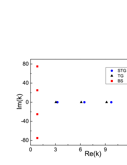
Figure 2: (Color online) The quasi momentum spectrum of $N=4$ bosons of TG, STG and Bound State branches for interaction constant $\left|\gamma\right|=50$.

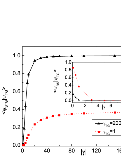
Figure 3: (Color online) The transition probability from TG branch to STG branch for $N=4$ bosons. The system is initially prepared in TG gas with $\gamma=200$ and Lieb-Lininger gas with $\gamma=1$. Inset shows the corresponding transition probability to the BS branch.

We show the energy spectrum of $N=4$ bosons for the three branches in the hard wall trap of width $L=1$ in Fig. 1. As in the case of homogeneous problem of three particles with periodic boundary conditions [27] and two particles in a harmonic trap [23, 28], the spectrum is quite different depending on the sign of the interaction parameter $\gamma$ or $c$ (we use $-1/\gamma$ in all figures in this paper). However, two matching points can be identified for the three solutions. In the non-interacting limit the ground states for the weakly repulsive (TG Branch) and weakly attractive (Bound State Branch) interacting systems join smoothly at the left and right end of the axis ($\gamma=0$) with $E/N=\pi^{2}/L^{2}$. On the other hand, in the strongly interacting limit the TG Branch adiabatically connects to the STG Branch at the origin of the axis ($-1/\gamma=0$) with energy $E/N=\pi^{2}(N+1)(2N+1)/6L^{2}$.

The solutions of quasi momentum $\left\{k_{j}\right\}$ for the three cases are presented in the complex plane of $k$ in Figure 2 for a large interacting parameter $\left|\gamma\right|=50$. The values are real for TG and STG branches, which become closer and closer when approaching the strong interacting point $-1/\gamma=0$. Unlike the case of periodic boundary condition [20], they are not any more symmetric about $k=0$. By assigning the initial value of $\left\{k_{j}\right\}$ a complex number, one obtains the string solutions for BS branch with a rather small real part and the imaginary parts lie symmetrically along the axis Im(k), indicating the conjugacy.

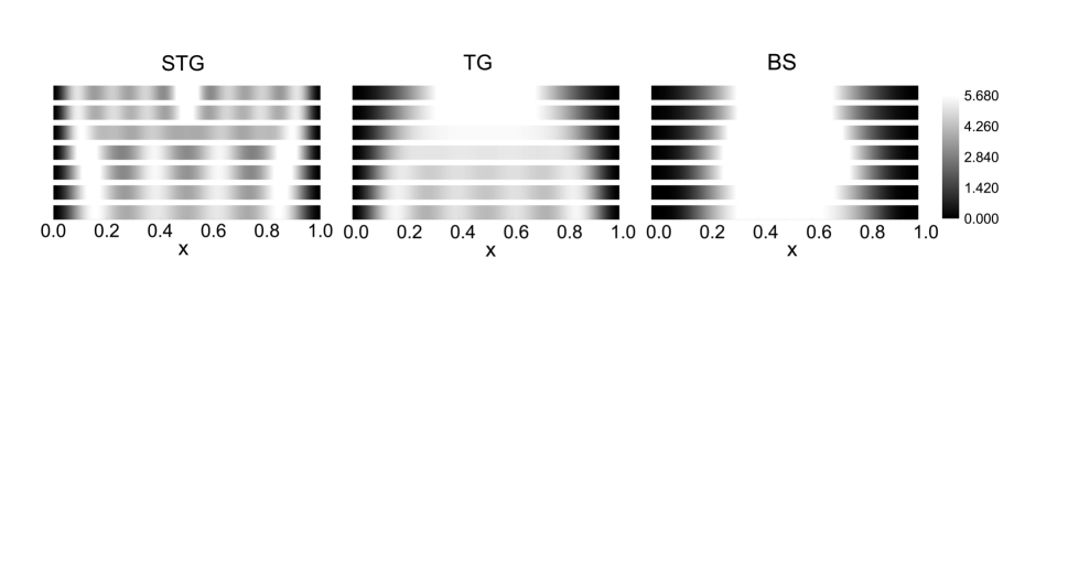
Figure 4: (Color online) The single particle density profiles for the three typical quantum phases of 1D interacting cold atoms. Left, middle and right panels show the gray scale plots for STG, TG and BS branches respectively, for seven gradually increasing interaction parameters and N = 4. Parameters from the top down are $\gamma=-0.1,-1,-2.5,-5,-12.5,-25,-100$ for STG, $\gamma=0.1,1,2.5,5,12.5,25,100$ for TG, and $\gamma=-0.1,-0.5,-1,-2,-3,-4,-5$ for the BS branches.

As shown in Figure 1, the energy changes smoothly from TG gas to STG gas when tuning the interaction parameter $-1/\gamma$ across the strongly interacting point from $-0$ to $+0$. This actually insures the deterministic preparation of the STG gas from the TG gas after a sudden change of interaction parameter via CIR. However, for the general case of an interacting bosonic system, this quench dynamics is complicated because the resulting state is a linear combination of eigenstates of the new Hamiltonian with $-1/\gamma>0$. The transition probability to other states, such as the bound states, is non-negligible for weakly interacting final state. Figure 3 shows the quenching dynamics of this interacting boson model, where the initial state is prepared in the TG Branch with $\gamma=200$ or $\gamma=1$, respectively. The transition probability to the final state in STG branch, characterized as $\left|\left\langle\Psi_{STG}\mid\Psi_{TG}\right\rangle\right|^{2}$, is plotted for varying parameter $\left|\gamma\right|$. The result confirms the metastable feature of the STG gas against collapsing into the bound state in the strongly attractive interaction regime. On the other hand, one has less probability to achieve the STG gas if the initial state is weakly repulsive. Inset in Figure 3 shows the transition probability to the bound state branch $\left|\left\langle\Psi_{BS}\mid\Psi_{TG}\right\rangle\right|^{2}$, for the same initial states. It is more likely that one will arrive at the bound state of small $\left|\gamma\right|$ if the system is initially prepared in the weakly interacting Lieb-Lininger gas.

Since single-particle density profiles normalized to $N$ depends crucially on the many-body wave function $\Psi$, one might anticipate to more easily recognize the distinction between the three quantum phases from their density distribution defined as

$$\rho\left(x\right)=N\int_{0}^{L}dx_{2}\cdots\int_{0}^{L}dx_{N}\left|\Psi\left(x,x_{2}\cdots,x_{N}\right)\right|^{2}.$$ (6)

Physically, $\rho\left(x\right)$ represents the probability that the bosons occupy the position $x$, which is accessible experimentally by means of the time of flight imaging technique. The single-particle density profiles for the three branches solution are illustrated in gray scale plot in Figure 4 for several gradually increasing interaction parameters and $N=4$. The left panel shows that in the excited state of STG branch the density of weakly interacting bosons exhibits seven peaks due to the slightly attraction between atoms, which develops gradually into four in the bottom plot when approaching the strong interacting STG regime. The density in the ground state of repulsive interacting bosons evolves in a quite different way as shown in the middle panel, however, merges into an identical four-peak structure in the strongly interacting point. This feature indicates the fermionization of bosonic atoms for either repulsive or attractive interaction for large value of $\left|\gamma\right|$. On the right panel, atoms in the ground bound state display always in a single peak, even for very large interaction parameter. We observe again the two matching points at $\gamma=0$ and $-1/\gamma=0$, as can be easily seen from the almost identical profiles at the bottom two plots of STG and TG branches and those at the top two plots of TG and BS branches.

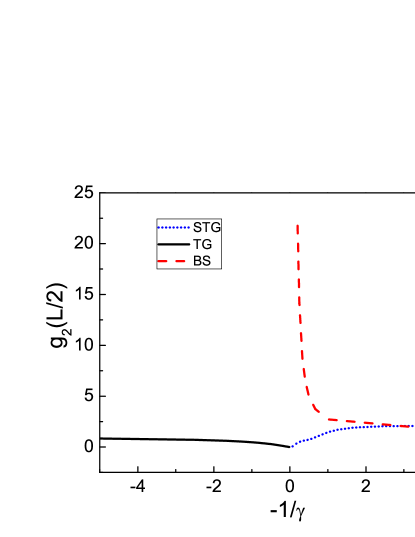
Figure 5: (Color online) The two-particle correlation function of TG, STG and Bound State branches in unit of $g_{2}\left(L/2,\gamma=0\right)$.

Another interesting feature of 1D exactly solvable model is the two-particle correlation function defined as

$$g_{2}\left(x\right) = N\left(N-1\right)\int_{0}^{L}dx_{3}\cdots\int_{0}^{L}dx_{N}$$ (7)

$$\times\left|\Psi\left(x,x,x_{3}\cdots,x_{N}\right)\right|^{2},$$

which may be used to identify and classify the quantum phases of 1D Bose gas. It is of particular importance for the studies of coherence properties of atom lasers produced in 1D waveguide. $g_{2}\left(x\right)$ denotes the probability that two successive measurements will find an atom at the same position $x$. The factor of $N(N-1)$ in Eq. (7) reflects there are $N(N-1)$ ways of choosing the $N-2$ integral variables out of $N$, just as we have $N$ ways of choosing the $N-1$ integral variables out of $N$ in the density distribution Eq. (6). In the Fig. 5, we show the two particle correlation function for 4 bosons in the position $x=L/2$ by numerically solving the Bethe Ansatz equations and doing the multiple integral for wave functions. We emphasize that the method used here is different from the approach in [20], where the correlation function has been obtained by numerically solving the integral equation in the thermodynamic limit. It can be perceived that generally the STG branch is more strongly correlated than the TG branch, especially $g_{2}(L/2)=2$ for very small value of $\left|\gamma\right|$. At the strong interacting point, the correlation vanishes for both STG and TG branches, $g_{2}(L/2)=0$, in agreement with the result of periodic boundary condition in thermodynamic limit [20]. On the contrary, the correlation function for the ground bound state with strong attractive interaction is significantly larger than the STG and TG gas, while it decreases rapidly to the result of non-interacting system, $g_{2}(L/2)=1$.

In summary, we have theoretically studied the ground state and excited state of a 1D Bose gas with arbitrary interaction strength in a hard wall trap. We show in the energy phase diagram the three quantum phases TG, STG and BS are closely connected to each other in the weakly and strongly interacting limits. We also calculate the density distribution and correlation function in the above cases and conclude that the STG gas is a strongly correlated state.

- [1] \NameM. A. Cazalilla, R. Citro, T. Giamarchi, E. Orignac M. Rigol \REVIEWarxiv1101.53372011.
- [2] \NameM. Olshanii \REVIEWPhy. Rev. Lett811998938.
- [3] \NameT. Bergeman, M. G. Moore M. Olshanii \REVIEWPhy. Rev. Lett912003163201.
- [4] \NameS. Sinha L. Santos \REVIEWPhy. Rev. Lett992007140406.
- [5] \Name T. Kinoshita, T. Wenger D. S. Weiss \REVIEWScience30520041125.
- [6] \NameB. Paredes, A. Widera, V. Murg, O. Mandel, S. Fölling, I. Cirac,G. V. Shlyapnikov, T. W. Hänsch I. Bloch \REVIEWNature (London)4292004277 .
- [7] \Name M. Girardeau \REVIEW J. Math. Phys11960516.
- [8] \Name J. Goold Th. Busch \REVIEWPhys. Rev. A772008063601.
- [9] \NameX. Lü, X. Yin Y. Zhang \REVIEWPhys. Rev. A812010043607.
- [10] \NameX. Yin, S. Chen Y. Zhang \REVIEWPhys. Rev. A792009053604.
- [11] \NameK. Lelas, D. Jukic H. Buljan \REVIEWPhys. Rev. A802009053617.
- [12] \NameF. Deuretzbacher, K. Bongs, K. Sengstock D. Pfannkuche \REVIEWPhys. Rev. A752007013614.
- [13] \NameS. Zöllner, H.-D. Meyer P. Schmelcher \REVIEWPhys. Rev. A742006053612.
- [14] \NameY. Hao, Y. Zhang, J.-Q. Liang S. Chen \REVIEWPhys. Rev. A732006063617.
- [15] \NameE. Haller, M. Gustavssn, M J. Mark, J. G. Danzl, R. Hart, G.Pupillo H.-C. Nägerl \REVIEWScience32520091224.
- [16] \NameJ. B. McGuire \REVIEWJ. Math. Phys51964622.
- [17] \NameE. Tempfi, S. Zöllner P. Schelcher \REVIEWPhys. Rev. Lett1052010150403.
- [18] \NameG. E. Astrakharchik, J. Boronat. J. Casulleras S. Giorgini \REVIEWPhy. Rev. Lett952005190407.
- [19] \Name M. T. Batchelor, M. Bortz, X. W. Guan N. Oelkers \REVIEWJ. Stat. Mech2005L1001.
- [20] \NameS. Chen, L. Guan, X. Yin, Y. Hao X.-W. Guan \REVIEWPhys. Rev. A812010031609(R).
- [21] \NameS. Chen, X.-W. Guan, X. Yin, L. Guan M. T. Batchelor \REVIEWPhys. Rev. A812010031608(R).
- [22] \NameE. H. Lieb W. Lininger \REVIEWPhys. Rev13019631605.
- [23] \NameT. Busch, B. Englert, K. Rzazewski M. Wilkens \REVIEWFound. Phys281998549.
- [24] \NameM. D. Girardeau G. E. Astrakharchik \REVIEWPhys. Rev. A812010061601.
- [25] \NameM. Gaudin \REVIEWPhys. Rev. A41971386
- [26] \NameK. Sakmann, A. I. Streltsov, O. E. Alon L. S. Cederbaum \REVIEWPhys. Rev. A722005033613.
- [27] \NameJ. G. Muga R. F. Snider \REVIEWPhys. Rev. A5719983317.
- [28] \NameD. Muth M. Fleischhauer \REVIEWPhys. Rev. Lett1052010150403.