Default Swap Games Driven by Spectrally Negative LÉvy Processes^∗

Abstract.

This paper studies game-type credit default swaps that allow the protection buyer and seller to raise or reduce their respective positions once prior to default. This leads to the study of an optimal stopping game subject to early default termination. Under a structural credit risk model based on spectrally negative Lévy processes, we apply the principles of smooth and continuous fit to identify the equilibrium exercise strategies for the buyer and the seller. We then rigorously prove the existence of the Nash equilibrium and compute the contract value at equilibrium. Numerical examples are provided to illustrate the impacts of default risk and other contractual features on the players’ exercise timing at equilibrium.

Keywords:  optimal stopping games; Nash equilibrium; Lévy processes; scale function; credit default swaps
JEL Classification:  C73, G13, G33, D81
Mathematics Subject Classification (2010):  91A15, 60G40, 60G51, 91B25

1. Introduction

Credit default swaps (CDSs) are among the most liquid and widely used credit derivatives for trading and managing default risks. Under a vanilla CDS contract, the protection buyer pays a periodic premium to the protection seller in exchange for a payment if the reference entity defaults before expiration. In order to control the credit risk exposure, investors can adjust the premium and notional amount prior to default by appropriately combining a market-traded default swaption with a vanilla CDS position, or use the over-the-counter traded products such as the callable CDSs (see [9, Chapter 21]). In a recent related work [27], we studied the optimal timing to step up or down a CDS position under a general Lévy credit risk model.

The current paper studies the game-type CDSs that allow both the protection buyer and seller to change the swap position once prior to default. Specifically, in the step-up (resp. step-down) default swap game, as soon as the buyer or the seller, whoever first, exercises prior to default, the notional amount and premium will be increased (resp. decreased) to a pre-specified level upon exercise. From the exercise time till default, the buyer will pay the new premium and the seller is subject to the new default liability. Hence, for a given set of contract parameters, the buyer’s objective is to maximize the expected net cash flow while the seller wants to minimize it, giving rise to a two-player optimal stopping game.

We model the default time as the first passage time of a general exponential Lévy process representing some underlying asset value. The default event occurs either when the underlying asset value moves continuously to the lower default barrier, or when it jumps below the default barrier. This is an extension of the original structural credit risk approach introduced by Black and Cox [8] where the asset value follows a geometric Brownian motion. As is well known [13], the incorporation of unpredictable jump-to-default is useful for explaining a number of market observations, such as the non-zero short-term limit of credit spreads. Other related credit risk models based on Lévy and other jump processes include [10, 19, 34].

The default swap game is formulated as a variation of the standard optimal stopping games in the literature (see, among others, [14, 17] and references therein). However, while typical optimal stopping games end at the time of exercise by either player, the exercise time in the default swap game does not terminate the contract, but merely alters the premium forward and the future protection amount to be paid at default time. In fact, since default may arrive before either party exercises, the game may be terminated early involuntarily.

The central challenge of the default swap games lies in determining the pair of stopping times that yield the Nash equilibrium. Under a structural credit risk model based on spectrally negative Lévy processes, we analyze and calculate the equilibrium exercise strategies for the protection buyer and seller. In addition, we determine the equilibrium premium of the default swap game so that the expected discounted cash flows for the two parties coincide at contract inception.

Our solution approach starts with a decomposition of the default swap game into a combination of a perpetual CDS and an optimal stopping game with early termination from default. Moreover, we utilize a symmetry between the step-up and step-down games, which significantly simplifies our analysis as it is sufficient to study either case. For a general spectrally negative Lévy process (with a non-atomic Lévy measure), we provide the conditions for the existence of the Nash equilibrium. Moreover, we derive the buyer’s and seller’s optimal threshold-type exercise strategies using the principle of continuous and smooth fit, followed by a rigorous verification theorem via martingale arguments.

For our analysis of the game equilibrium, the scale function and a number of fluctuation identities of spectrally negative Lévy processes are particularly useful. Using our analytic results, we provide a bisection-based algorithm for the efficient computation of the buyer’s and seller’s exercise thresholds as well as the equilibrium premium, illustrated in a series of numerical examples. Other recent applications of spectrally negative Lévy processes include derivative pricing [1, 2], optimal dividend problem [3, 24, 29], and capital reinforcement timing [16]. We refer the reader to [23] for a comprehensive account.

To our best knowledge, the step-up and step-down default swap games and the associated optimal stopping games have not been studied elsewhere. There are a few related studies on stochastic games driven by spectrally negative or positive Lévy processes; see e.g. [4] and [5]. For optimal stopping games driven by a strong Markov process, we refer to the recent papers by [17] and [31], which study the existence and mathematical characterization of Nash equilibrium. Other game-type derivatives in the literature include Israeli/game options [21, 22], defaultable game options [6], and convertible bonds [20, 33].

The rest of the paper is organized as follows. In Section 2, we formulate the default swap game under a general Lévy model. In Section 3, we focus on the spectrally negative Lévy model and analyze the Nash equilibrium. Section 4 provides the numerical study of the default swap games for the case with i.i.d. exponential jumps. Section 5 concludes the paper and presents some ideas for future work. All proofs are given in the Appendix.

2. Game Formulation

On a complete probability space $(\Omega,\mathcal{F},\mathbb{P})$, we assume there exists a Lévy process $X=\{X_{t};\,t\geq 0\}$ and denote by $\mathbb{F}=(\mathcal{F}_{t})_{t\geq 0}$ the filtration generated by $X$. The value of the reference entity (a company stock or other assets) is assumed to evolve according to an exponential Lévy process $S_{t}=e^{X_{t}}$, $t\geq 0$. Following the Black-Cox [8] structural approach, the default event is triggered by $S$ crossing a lower level $D$. Without loss of generality, we can take $\log D=0$ by shifting the initial value $x\in\mathbb{R}$. Henceforth, we shall work with the default time

$${\sigma_{0}}:=\inf\{\,t\geq 0\,:\,X_{t}\,\leq\,0\,\},$$

where $\inf\emptyset\!=\!\infty$ by convention. We denote by $\mathbb{P}^{x}$ the probability law and $\mathbb{E}^{x}$ the expectation with $X_{0}=x$.

We consider a default swap contract that gives the protection buyer and seller an option to change the premium and notional amount before default for a fee, whoever exercises first. Specifically, the buyer begins by paying premium at rate $p$ over time for a notional amount $\alpha$ to be paid at default. Prior to default, the buyer and the seller can select a time to switch to a new premium $\hat{p}$ and notional amount $\hat{\alpha}$. When the buyer exercises, she is incurred the fee $\gamma_{b}$ to be paid to the seller; when the seller exercises, she is incurred $\gamma_{s}$ to be paid to the buyer. If the buyer and the seller exercise simultaneously, then both parties pay the fee upon exercise. We assume that $p$, $\hat{p}$, $\alpha$, $\hat{\alpha}$, $\gamma_{b}$, $\gamma_{s}\geq 0$ (see also Remark 2.2 below).

Let $\mathcal{S}:=\left\{\tau\in\mathbb{F}:\tau\leq{\sigma_{0}}\;\text{ a.s. }\right\}$ be the set of all stopping times smaller than or equal to the default time. Denote the buyer’s candidate exercise time by $\tau\in\mathcal{S}$ and seller’s candidate exercise time by $\sigma\in\mathcal{S}$, and let $r>0$ be the positive risk-free interest rate. Given any pair of exercise times $(\sigma,\tau)$, the expected cash flow to the buyer is given by

$$V(x;\sigma,\tau):=\mathbb{E}^{x}\left[-\int_{0}^{\tau\wedge\sigma}e^{-rt}p\,{\rm d}t+1_{\{\tau\wedge\sigma<\infty\}}\bigg{(}-\int_{\tau\wedge\sigma}^{\sigma_{0}}e^{-rt}\hat{p}\,{\rm d}t\right.\\ \left.+e^{-r{\sigma_{0}}}(\hat{\alpha}1_{\{{\tau\wedge\sigma}<{\sigma_{0}}\}}+\alpha 1_{\{{\tau\wedge\sigma}={\sigma_{0}}\}})+1_{\{\tau\wedge\sigma<{\sigma_{0}}\}}e^{-r(\tau\wedge\sigma)}\left(-\gamma_{b}1_{\{\tau\leq\sigma\}}+\gamma_{s}1_{\{\tau\geq\sigma\}}\right)\bigg{)}\right].$$ (2.1)

To the seller, the contract value is $-V(x;\sigma,\tau)$. Naturally, the buyer wants to maximize $V$ over $\tau$ whereas the seller wants to minimize $V$ over $\sigma$, giving rise to a two-player optimal stopping game.

This formulation covers default swap games with the following provisions:

1. Step-up Game: if $\hat{p}>p$ and $\hat{\alpha}>\alpha$, then the buyer and the seller are allowed to increase the notional amount once from $\alpha$ to $\hat{\alpha}$ and the premium rate from $p$ to $\hat{p}$ by paying the fee $\gamma_{b}$ (if the buyer exercises) or $\gamma_{s}$ (if the seller exercises).

2. Step-down Game: if $\hat{p}<p$ and $\hat{\alpha}<\alpha$, then the buyer and the seller are allowed to decrease the notional amount once from $\alpha$ to $\hat{\alpha}$ and the premium rate from $p$ to $\hat{p}$ by paying the fee $\gamma_{b}$ (if the buyer exercises) or $\gamma_{s}$ (if the seller exercises). When $\hat{p}=\hat{\alpha}=0$, we obtain a cancellation game which allows the buyer and the seller to terminate the contract early.

Our primary objective is to determine the pair of stopping times $(\sigma^{*},\tau^{*})\subset\mathcal{S}$, called the saddle point, that constitutes the Nash equilibrium:

$$V(x;\sigma^{*},\tau)\leq V(x;\sigma^{*},\tau^{*})\leq V(x;\sigma,\tau^{*}),\quad\forall\,\sigma,\tau\in\mathcal{S}.$$ (2.2)

Remark 2.1.

A related concept is the Stackelberg equilibrium, represented by the equality $V^{*}(x)=V_{*}(x)$, where $V^{*}(x):=\inf_{\sigma\in\mathcal{S}}\sup_{\tau\in\mathcal{S}}V(x;\sigma,\tau)$ and $V_{*}(x):=\sup_{\tau\in\mathcal{S}}\inf_{\sigma\in\mathcal{S}}V(x;\sigma,\tau)$. See e.g. [17] and [31]. These definitions imply that $V^{*}(x)\geq V_{*}(x)$. The existence of the Nash equilibrium (2.2) will also yield the Stackelberg equilibrium via the reverse inequality:

$$V^{*}(x)\leq\sup_{\tau\in\mathcal{S}}V(x;\sigma^{*},\tau)\leq V(x;\sigma^{*},\tau^{*})\leq\inf_{\sigma\in\mathcal{S}}V(x;\sigma,\tau^{*})\leq V_{*}(x).$$

Herein, we shall focus our analysis on the Nash equilibrium.

Our main results on the Nash equilibrium are summarized in Theorems 3.1-3.2 for the spectrally negative Lévy case. As preparation, we begin our analysis with two useful observations, namely, the decomposition of $V$ and the symmetry between the step-up and step-down games.

2.1. Decomposition and Symmetry

In standard optimal stopping games, such as the well-known Dynkin game [14], random payoffs are realized at either player’s exercise time. However, our default swap game is not terminated at the buyer’s or seller’s exercise time. In fact, upon exercise only the contract terms will change, and there will be a terminal transaction at default time. Since default may arrive before either party exercises the step-up/down option, the game may be terminated early involuntarily. Therefore, we shall transform the value function $V$ into another optimal stopping game that is more amenable for analysis.

First, we define the value of a (perpetual) CDS with premium rate $p$ and notional amount $\alpha$ by

$$C(x;p,\alpha) :=\mathbb{E}^{x}\left[-\int_{0}^{{\sigma_{0}}}e^{-rt}p\,{\rm d}t+\alpha\,e^{-r{\sigma_{0}}}\right]=\left(\frac{p}{r}+\alpha\right)\zeta(x)-\frac{p}{r},\quad x>0,$$ (2.3)

where

$$\zeta(x):=\mathbb{E}^{x}\left[e^{-r{\sigma_{0}}}\right],\quad x\in\mathbb{R},$$ (2.4)

is the Laplace transform of ${\sigma_{0}}$. Next, we extract this CDS value from the value function $V$. Let

$$\tilde{\alpha}:=\alpha-\hat{\alpha}\quad\textrm{and}\quad\tilde{p}:=p-\hat{p}.$$ (2.5)

Proposition 2.1 (decomposition).

For every $\sigma,\tau\in\mathcal{S}$ and $x>0$, the value function admits the decomposition

$$V(x;\sigma,\tau) =C(x;p,\alpha)+v(x;\sigma,\tau),$$

where $v(x;\sigma,\tau)\equiv v(x;\sigma,\tau;\tilde{p},\tilde{\alpha},\gamma_{b},\gamma_{s})$ is defined by

$$v(x;\sigma,\tau;\tilde{p},\tilde{\alpha},\gamma_{b},\gamma_{s}):=\mathbb{E}^{x}\left[e^{-r(\tau\wedge\sigma)}\left(h(X_{\tau})1_{\{\tau<\sigma\}}+g(X_{\sigma})1_{\{\tau>\sigma\}}+f(X_{\tau})1_{\{\tau=\sigma\}}\right)1_{\{\tau\wedge\sigma<\infty\}}\right],$$ (2.6)

with

$$h(x) \equiv h(x;\tilde{p},\tilde{\alpha},\gamma_{b}):=1_{\{x>0\}}\Big{[}\Big{(}\frac{\tilde{p}}{r}-\gamma_{b}\Big{)}-\Big{(}\frac{\tilde{p}}{r}+\tilde{\alpha}\Big{)}\zeta(x)\Big{]},$$ (2.7)

$$g(x) \equiv g(x;\tilde{p},\tilde{\alpha},\gamma_{s}):=1_{\{x>0\}}\Big{[}\Big{(}\frac{\tilde{p}}{r}+\gamma_{s}\Big{)}-\Big{(}\frac{\tilde{p}}{r}+\tilde{\alpha}\Big{)}\zeta(x)\Big{]},$$ (2.8)

$$f(x) \equiv f(x;\tilde{p},\tilde{\alpha},\gamma_{b},\gamma_{s}):=1_{\{x>0\}}\Big{[}\Big{(}\frac{\tilde{p}}{r}-\gamma_{b}+\gamma_{s}\Big{)}-\Big{(}\frac{\tilde{p}}{r}+\tilde{\alpha}\Big{)}\zeta(x)\Big{]}.$$ (2.9)

Comparing (2.3) and (2.7), we see that $h(x)=1_{\{x>0\}}(C(x;-\tilde{p},-\tilde{\alpha})-\gamma_{b})$, which means that the buyer receives the CDS value $C(x;-\tilde{p},-\tilde{\alpha})$ at the cost of $\gamma_{b}$ if she exercises before the seller. For the seller, the payoff of exercising before the buyer is $-g(x)=1_{\{x>0\}}(C(x;\tilde{p},\tilde{\alpha})-\gamma_{s})$. Hence, in both cases the fees $\gamma_{b}$ and $\gamma_{s}$ can be viewed as strike prices.

Since $C(x;p,\alpha)$ does not depend on $(\sigma,\tau)$, Proposition 2.1 implies that finding the saddle point $(\sigma^{*},\tau^{*})$ for the Nash equilibrium in (2.2) is equivalent to showing that

$$v(x;\sigma^{*},\tau)\leq v(x;\sigma^{*},\tau^{*})\leq v(x;\sigma,\tau^{*}),\quad\forall\,\sigma,\tau\in\mathcal{S}.$$ (2.10)

If the Nash equilibrium exists, then the value of the game is $V(x;\sigma^{*},\tau^{*})=C(x)+v(x;\sigma^{*},\tau^{*})$, $x\in\mathbb{R}.$ According to (2.5), the problem is a step-up (resp. step-down) game when $\tilde{\alpha}<0$ and $\tilde{p}<0$ (resp. $\tilde{\alpha}>0$ and $\tilde{p}>0$).

Remark 2.2.

If $\gamma_{b}=\gamma_{s}=0$, then it follows from (2.7)-(2.9) that $h(x)=g(x)=f(x)$ and

$$v(x;\sigma,\tau;\tilde{p},\tilde{\alpha},0,0)=\mathbb{E}^{x}\left[e^{-r(\tau\wedge\sigma)}1_{\{X_{\tau\wedge\sigma}>0,\,\tau\wedge\sigma<\infty\}}C(X_{\tau\wedge\sigma};-\tilde{p},-\tilde{\alpha})\right].$$

In this case, the choice of $\tau^{*}=\sigma^{*}=0$ yields the equilibrium (2.10) with equalities, so the default swap game is always trivially exercised at inception by either party. For similar reasons, we also rule out the trivial case with $\tilde{p}=0$ or $\tilde{\alpha}=0$ (even with $\gamma_{s}+\gamma_{b}>0$). Furthermore, we ignore the contract specifications with $\tilde{p}\tilde{\alpha}<0$ since they mean paying more (resp. less) premium in exchange for a reduced (resp. increased) protection after exercise. Henceforth, we proceed our analysis with $\tilde{p}\tilde{\alpha}>0$ and $\gamma_{b}+\gamma_{s}>0$.

Next, we observe the symmetry between the step-up and step-down games.

Proposition 2.2 (symmetry).

For any $\sigma,\tau\in\mathcal{S}$, we have $v(x;\sigma,\tau;\tilde{p},\tilde{\alpha},\gamma_{b},\gamma_{s})=-v(x;\tau,\sigma;-\tilde{p},-\tilde{\alpha},\gamma_{s},\gamma_{b})$.

Applying Proposition 2.2 to the Nash equilibrium condition (2.10), we deduce that if $(\sigma^{*},\tau^{*})$ is the saddle point for the step-down default swap game with $(\tilde{p},\tilde{\alpha},\gamma_{b},\gamma_{s})$, then the reversed pair $(\tau^{*},\sigma^{*})$ is the saddle point for the step-up default swap game with $(-\tilde{p},-\tilde{\alpha},\gamma_{s},\gamma_{b})$. Consequently, the symmetry result implies that it is sufficient to study either the step-down or the step-up default swap game. This significantly simplifies our analysis. Henceforth, we solve only for the step-down game.

Also, we notice from (2.1) that if $\tilde{\alpha}\leq\gamma_{s}$, then the seller’s benefit of a reduced exposure does not exceed the fee, and therefore, should never exercise. As a result, the valuation problem is reduced to a step-down CDS studied in [27], and so we exclude it from our analysis here. With this observation and Remark 2.2, we will proceed with the following assumption without loss of generality:

Assumption 2.1.

We assume that $\tilde{\alpha}>\gamma_{s}\geq 0$, $\tilde{p}>0$ and $\gamma_{b}+\gamma_{s}>0$.

2.2. Candidate Threshold Strategies

In the step-down game, the protection buyer has an incentive to step-down when default is less likely, or equivalently when $X$ is sufficiently high. On the other hand, the protection seller tends to exercise the step-down option when default is likely to occur, or equivalently when $X$ is sufficiently small. This intuition leads us to conjecture the following threshold strategies, respectively, for the buyer and the seller:

$$\tau_{B}:=\inf\left\{t\geq 0:X_{t}\notin(0,B)\right\},\quad\text{and}\quad\sigma_{A}:=\inf\left\{t\geq 0:X_{t}\notin(A,\infty)\right\},$$

for $B>A>0$. Clearly, $\sigma_{A},\tau_{B}\in\mathcal{S}$. For $B>A>0$, we denote the candidate value function

$$v_{A,B}(x) :=v(x;\sigma_{A},\tau_{B})$$

$$=\mathbb{E}^{x}\left[e^{-r(\tau_{B}\wedge\sigma_{A})}\left(h(X_{\tau_{B}})1_{\{\tau_{B}<\sigma_{A}\}}+g(X_{\sigma_{A}})1_{\{\tau_{B}>\sigma_{A}\}}+f(X_{\tau_{B}})1_{\{\tau_{B}=\sigma_{A}\}}\right)1_{\{\tau_{B}\wedge\sigma_{A}<\infty\}}\right]$$

$$=\mathbb{E}^{x}\left[e^{-r(\tau_{B}\wedge\sigma_{A})}\left(h(X_{\tau_{B}})1_{\{\tau_{B}<\sigma_{A}\}}+g(X_{\sigma_{A}})1_{\{\tau_{B}>\sigma_{A}\}}\right)1_{\{\tau_{B}\wedge\sigma_{A}<\infty\}}\right]$$ (2.11)

for every $x\in\mathbb{R}$. The last equality follows since $\tau_{B}=\sigma_{A}$ implies that $\tau_{B}=\sigma_{A}={\sigma_{0}}$, and $f(X_{\sigma_{0}})=0$ a.s.

In subsequent sections, we will identify the candidate exercise thresholds $A^{*}$ and $B^{*}$ simultaneously by applying the principle of continuous and smooth fit:

$$(\text{continuous fit})\quad v_{A,B}(B-)-h(B) =0\quad\text{and}\quad v_{A,B}(A+)-g(A)=0,$$ (2.12)

$$(\text{smooth fit})\quad v_{A,B}^{\prime}(B-)-h^{\prime}(B) =0\quad\text{and}\quad v^{\prime}_{A,B}(A+)-g^{\prime}(A)=0,$$ (2.13)

if these limits exist.

3. Solution Methods for the Spectrally Negative Lévy Model

We now define $X$ to be a spectrally negative Lévy process with the Laplace exponent

$$\phi(s):=\log\mathbb{E}^{0}\left[e^{sX_{1}}\right]=cs+\frac{1}{2}\nu^{2}s^{2}+\int_{(0,\infty)}(e^{-su}-1+su1_{\{0<u<1\}})\,\Pi({\rm d}u),\quad{s\in\mathbb{R}},$$ (3.1)

where $c\in\mathbb{R}$, $\nu\geq 0$ is called the Gaussian coefficient, and $\Pi$ is a Lévy measure on $(0,\infty)$ such that
$\int_{(0,\infty)}(1\wedge u^{2})\Pi({\rm d}u)<\infty$. See [23, p.212]. It admits a unique decomposition:

$$X=X^{c}+X^{d}$$ (3.2)

where $X^{c}$ is the continuous martingale (Brownian motion) part and $X^{d}$ is the jump and drift part of $X$. Moreover,

$$\textrm{$X^{d}$ has paths of bounded variation}\Longleftrightarrow\int_{0}^{1}u\Pi({\rm d}u)<\infty.$$ (3.3)

If this condition (3.3) is satisfied, then the Laplace exponent simplifies to

$$\phi(s)=\mu s+\frac{1}{2}\nu^{2}s^{2}+\int_{(0,\infty)}(e^{-su}-1)\,\Pi({\rm d}u),\quad s\in\mathbb{C},$$ (3.4)

where $\mu:=c+\int_{(0,1)}u\,\Pi({\rm d}u)$. Recall that $X$ has paths of bounded variation if and only if $\nu=0$ and (3.3) holds. We ignore the case when $X$ is a negative subordinator (decreasing a.s.). This means that we require $\mu$ to be strictly positive if $\nu=0$ and (3.3) holds. We also assume the following and also Assumption 3.2 below.

Assumption 3.1.

We assume that the Lévy measure $\Pi$ does not have atoms.

3.1. Main Results

We now state our main results concerning the Nash equilibrium and its associated saddle point. We will identify the pair of thresholds $(A^{*},B^{*})$ for the seller and buyer at equilibrium. The first theorem considers the case $A^{*}>0$, where the seller exercises at a level strictly above zero.

Theorem 3.1.

Suppose $A^{*}>0$. The Nash equilibrium exists with saddle point $(\sigma_{A^{*}},\tau_{B^{*}})$ satisfying

$$v(x;\sigma_{A^{*}},\tau)\leq v_{A^{*},B^{*}}(x)\leq v(x;\sigma,\tau_{B^{*}}),\quad\forall\sigma,\tau\in\mathcal{S}.$$ (3.5)

Here $v_{A^{*},B^{*}}(x)\equiv v(x;\sigma_{A^{*}},\tau_{B^{*}})$ as in (2.11) and can be expressed in terms of the scale function as we shall see in Subsection 3.2. In particular, the case $B^{*}=\infty$ reflects that $\tau_{B^{*}}=\sigma_{0}$ and $v_{A^{*},\infty}(x):=\lim_{B\uparrow\infty}v_{A^{*},B}(x)$ is the expected value when the buyer never exercises and the seller’s strategy is $\tau_{A^{*}}$. The value function can be computed using (3.21) and (3.30) below.

The case $A^{*}=0$ may occur, which is more technical and may not yield the Nash equilibrium. To see why, we notice that a default happens as soon as $X$ touches zero. Therefore, in the event that $X$ continuously passes (creeps) through zero, the seller would optimally seek to exercise at a level as close to zero as possible. Nevertheless, this timing strategy is not admissible, though it can be approximated arbitrarily closely by admissible stopping times.

As shown in Corollary 3.1 below, the case $A^{*}=0$ is possible only if the jump part $X^{d}$ of $X$ is of bounded variation (see (3.3)). This is consistent with our intuition because if $X$ jumps downward frequently, then the seller has the incentive to step down the position at a level strictly above zero. On the other hand, when $\nu=0$ (with no Gaussian component), the process $X$ never goes through continuously the level zero, so even with $A^{*}=0$ the Nash equilibrium in Theorem 3.1 still holds. In contrast, if $\nu>0$, then an alternative form of “equilibrium” is attained, namely,

$$v(x;\sigma_{0+},\tau)\leq v_{0+,B^{*}}(x)\leq v(x;\sigma,\tau_{B^{*}}),\quad\forall\sigma,\tau\in\mathcal{S},$$ (3.6)

where

$$v(x;\sigma_{0+},\tau) :=\mathbb{E}^{x}\left[e^{-r\tau}(h(X_{\tau})-(\tilde{\alpha}-\gamma_{s})1_{\{X_{\tau}=0\}})1_{\{\tau<\infty\}}\right],\quad\tau\in\mathcal{S},$$

$$v_{0+,B^{*}}(x) :=\mathbb{E}^{x}\big{[}e^{-r\tau_{B^{*}}}(h(X_{\tau_{B^{*}}})-(\tilde{\alpha}-\gamma_{s})1_{\{X_{\tau_{B^{*}}}=0\}})1_{\{\tau_{B^{*}}<\infty\}}\big{]}.$$

Here, the functions $v(x;\sigma_{0+},\tau)$ and $v_{0+,B^{*}}(x)$ correspond to the limiting case where the seller exercises arbitrarily close to the default time $\sigma_{0}$. However, since the seller cannot predict the default time, this timing strategy is not admissible and (3.6) is not the Nash equilibrium. In practice, given the buyer’s strategy $\tau_{B^{*}}$, the seller’s value function can be approximated with an $\varepsilon$-optimal strategy by choosing $\sigma_{\delta}$ for a sufficiently low exercise level $\delta>0$.

Let us summarize our equilibrium results for the case $A^{*}=0$.

Theorem 3.2.

For the case $A^{*}=0$,

1. if $\nu=0$, a Nash equilibrium exists with saddle point $({\sigma_{0}},\tau_{B^{*}})$ and (3.5) holds;

2. if $\nu>0$, then the alternative equilibrium (3.6) holds.

In the remainder of this section, we take the following steps to prove the existence of $(A^{*},B^{*})$ and Theorems 3.1-3.2:

1. In Section 3.2, we express the candidate value function $v_{A,B}$ in terms of the Lévy scale function.

2. In Section 3.3, we establish the sufficient conditions for continuous and smooth fit.

3. In Section 3.4, we show the existence of the candidate optimal thresholds $A^{*}$ and $B^{*}$ (Theorem 3.3).

4. In Section 3.5, we verify the optimality of the candidate optimal exercise strategies.

Furthermore, in Section 3.4 we provide an efficient algorithm to compute the pair $(A^{*},B^{*})$ and $v_{A^{*},B^{*}}(x)$. Finally, with Theorems 3.1-3.2, the value of the step-down game is recovered by $V(x)=C(x)+v(x)$ by Proposition 2.1 and that of the step-up game is recovered by $V(x)=C(x)-v(x)$ by Proposition 2.2.

Remark 3.1.

For the fair valuation of the default swap game, one may specify $\mathbb{P}$ as the risk-neutral pricing measure. The risk-neutrality condition would require that $\phi(1)=r$ so that the discounted asset value is a $(\mathbb{P},\mathbb{F})$-martingale. This condition is not needed for our solution approach and equilibrium results.

3.2. Expressing $v_{A,B}$ using the scale function.

In this subsection, we shall summarize the scale function associated with the process $X$, and then apply this to compute the candidate value function $v_{A,B}(x)$ defined in (2.11). For any spectrally negative Lévy process, there exists a function $W^{(r)}:\mathbb{R}\mapsto\mathbb{R}$, which is zero on $(-\infty,0)$ and continuous and strictly increasing on $[0,\infty)$. It is characterized by the Laplace transform:

$$\int_{0}^{\infty}e^{-sx}W^{(r)}(x){\rm d}x=\frac{1}{\phi(s)-r},\qquad s>\Phi(r),$$

where $\Phi$ is the right inverse of $\phi$, defined by

$$\Phi(r):=\sup\{\lambda\geq 0:\phi(\lambda)=r\}.$$

The function $W^{(r)}$ is often called the (r-)scale function in the literature (see e.g. [23]).

With $\Phi(r)$ and $W^{(r)}$, we can define the function $W_{\Phi(r)}=\{W_{\Phi(r)}(x);x\in\mathbb{R}\}$ by

$$W_{\Phi(r)}(x)=e^{-\Phi(r)x}W^{(r)}(x),\quad x\in\mathbb{R}.$$ (3.7)

As is well known (see [23, Chapter 8]), the function $W_{\Phi(r)}(x)$ is increasing, and satisfies

$$W_{\Phi(r)}(x) \uparrow\frac{1}{\phi^{\prime}(\Phi(r))}\quad\textrm{as }\;x\uparrow\infty.$$ (3.8)

From Lemmas 4.3-4.4 of [26], we also summarize the behavior of $W^{(r)}$ in the neighborhood of zero:

$$W^{(r)}(0)=\left\{\begin{array}[]{ll}0,&\textrm{unbounded variation}\\ \frac{1}{\mu},&\textrm{bounded variation}\end{array}\right\}\quad\textrm{and}\quad W^{(r)^{\prime}}(0+)=\left\{\begin{array}[]{ll}\frac{2}{\nu^{2}},&\nu>0\\ \infty,&\nu=0\;\textrm{and}\;\Pi(0,\infty)=\infty\\ \frac{r+\Pi(0,\infty)}{\mu^{2}},&\textrm{compound Poisson}\end{array}\right\}.$$ (3.14)

To facilitate calculations, we define the function

$$Z^{(r)}(x):=1+r\int_{0}^{x}W^{(r)}(y){\rm d}y,\quad x\in\mathbb{R}$$

which satisfies that

$$\frac{Z^{(r)}(x)}{W^{(r)}(x)}\xrightarrow{x\uparrow\infty}\frac{r}{\Phi(r)};$$ (3.15)

see [23] Exercise 8.5. By Theorem 8.5 of [23], the Laplace transform of ${\sigma_{0}}$ in (2.4) can be expressed as

$$\zeta(x)=Z^{(r)}(x)-\frac{r}{\Phi(r)}W^{(r)}(x),\quad x>0.$$ (3.16)

Regarding the smoothness of the scale function, Assumption 3.1 guarantees that $W^{(r)}(x)$ is differentiable on $(0,\infty)$ (see, e.g., [12]). By (3.16), Laplace transform function $\zeta$ is also differentiable on $(0,\infty)$, and so are the functions $h,g,f$ in (2.7)-(2.9). In this paper, we need the twice differentiability for the case of unbounded variation.

Assumption 3.2.

For the case $X$ is of unbounded variation, we assume that $W^{(r)}$ is twice differentiable on $(0,\infty)$.

This assumption is automatically satisfied if $\nu>0$ as in [12], and the same property holds for $\zeta,h,g$, and $f$. While this is not guaranteed for the unbounded variation case with $\nu=0$, it is an assumption commonly needed when the verification of optimality requires the infinitesimal generator.

Moreover, as in (8.18) of [23],

$$\frac{W^{(r)^{\prime}}(y)}{W^{(r)}(y)}\leq\frac{W^{(r)^{\prime}}(x)}{W^{(r)}(x)}\quad\textrm{and}\quad\frac{W^{{}^{\prime}}_{\Phi(r)}(y)}{W_{\Phi(r)}(y)}\leq\frac{W^{{}^{\prime}}_{\Phi(r)}(x)}{W_{\Phi(r)}(x)},\quad y>x>0,$$ (3.17)

and, using (3.8), we deduce that

$$\frac{W^{(r)^{\prime}}(x)}{W^{(r)}(x)}=\frac{\Phi(r)e^{\Phi(r)x}W_{\Phi(r)}(x)+e^{\Phi(r)x}W_{\Phi(r)}^{\prime}(x)}{e^{\Phi(r)x}W_{\Phi(r)}(x)}=\frac{\Phi(r)W_{\Phi(r)}(x)+W_{\Phi(r)}^{\prime}(x)}{W_{\Phi(r)}(x)}\xrightarrow{x\uparrow\infty}{\Phi(r)}.$$ (3.18)

In applying the scale function to compute $v_{A,B}(x)$, we first consider the case $0<A<B<\infty$ and then extend to the cases $A\downarrow 0$ and $B\uparrow\infty$, namely,

$$v_{A,\infty}(x):=\lim_{B\uparrow\infty}v_{A,B}(x)\quad\textrm{and}\quad v_{0+,B}(x):=\lim_{A\downarrow 0}v_{A,B}(x).$$ (3.19)

For $0<A<x<B<\infty$, define

$$\begin{split}\Upsilon(x;A,B)&:=\Big{(}\frac{\tilde{p}}{r}-\gamma_{b}\Big{)}\mathbb{E}^{x}\left[e^{-r(\sigma_{A}\wedge\tau_{B})}1_{\{\tau_{B}<\sigma_{A}\}}\right]+\Big{(}\frac{\tilde{p}}{r}+\gamma_{s}\Big{)}\mathbb{E}^{x}\left[e^{-r(\sigma_{A}\wedge\tau_{B})}1_{\{\tau_{B}>\sigma_{A}\,\textrm{or}\;\sigma_{A}\wedge\tau_{B}={\sigma_{0}}\}}\right]\\ &\;+(\tilde{\alpha}-\gamma_{s})\mathbb{E}^{x}\left[e^{-r(\sigma_{A}\wedge\tau_{B})}1_{\{\sigma_{A}\wedge\tau_{B}={\sigma_{0}}\}}\right].\end{split}$$ (3.20)

We observe that $v_{A,B}(x)-h(x)$ and $v_{A,B}(x)-g(x)$ are similar and they possess the common term $\Upsilon(x;A,B)$.

Lemma 3.1.

For $0<A<x<B<\infty$,

$$\begin{split}v_{A,B}(x)-h(x)&=\Upsilon(x;A,B)-\Big{(}\frac{\tilde{p}}{r}-\gamma_{b}\Big{)},\\ v_{A,B}(x)-g(x)&=\Upsilon(x;A,B)-\Big{(}\frac{\tilde{p}}{r}+\gamma_{s}\Big{)},\end{split}$$ (3.21)

and

$$\Upsilon(x;A,B) =W^{(r)}(x-A)\frac{\Psi(A,B)}{W^{(r)}(B-A)}+\Big{(}\frac{\tilde{p}}{r}+\gamma_{s}\Big{)}Z^{(r)}(x-A)-\left(\tilde{\alpha}-\gamma_{s}\right)\kappa(x;A),$$ (3.22)

where

$$\Psi(A,B) :=\Big{(}\frac{\tilde{p}}{r}-\gamma_{b}\Big{)}-\Big{(}\frac{\tilde{p}}{r}+\gamma_{s}\Big{)}Z^{(r)}(B-A)+\left(\tilde{\alpha}-\gamma_{s}\right)\kappa(B;A),\quad 0<A<B<\infty,$$ (3.23)

$$\begin{split}\kappa(x;A)&:=\int_{A}^{\infty}\Pi({\rm d}u)\int_{0}^{u\wedge x-A}{\rm d}zW^{(r)}(x-z-A)\\ &\;=\frac{1}{r}\int_{A}^{\infty}\Pi({\rm d}u)\left[Z^{(r)}(x-A)-Z^{(r)}(x-u)\right],\quad x>A>0.\end{split}$$ (3.24)

The function $\Psi(A,B)$ as in (3.23) will play a crucial role in the continuous and smooth fit as we discuss in Subsection 3.3 below and also in the proof of the existence of a pair $(A^{*},B^{*})$ as in Subsection 3.4.

Now we extend our definition of $v_{A,B}$ for $A=0+$ and $B=\infty$ as in (3.19), and then derive the strategies that attain them. As we shall see in Corollary 3.1 below, our candidate threshold level for the seller $A^{*}$ is always strictly positive if $X^{d}$ is of unbounded variation whether or not there is a Gaussian component. For this reason, we consider the limit as $A\downarrow 0$ only when (3.3) is satisfied.

In view of (3.21), the limits in (3.19) can be obtained by extending $\Upsilon(x;A,B)$ with $A\downarrow 0$ and $B\uparrow\infty$; namely we take limits in (3.22). Here $\Psi$ as in (3.23) explodes as $B\uparrow\infty$ and hence we define an extended version of ${\Psi(A,B)}/{W^{(r)}(B-A)}$ by, for any $0\leq A<B\leq\infty$ (with the assumption $\int_{0}^{1}u\Pi({\rm d}u)<\infty$ for $A=0$),

$$\widehat{\Psi}(A,B) :=\left\{\begin{array}[]{ll}\frac{1}{W^{(r)}(B-A)}\left[\left(\frac{\tilde{p}}{r}-\gamma_{b}\right)-\left(\frac{\tilde{p}}{r}+\gamma_{s}\right)Z^{(r)}(B-A)+\left(\tilde{\alpha}-\gamma_{s}\right)\kappa(B;A)\right],&B<\infty,\\ \frac{1}{\Phi(r)}\left(-(\tilde{p}+r\gamma_{s})+(\tilde{\alpha}-\gamma_{s})\rho(A)\right),&B=\infty,\end{array}\right.$$ (3.27)

where

$$\rho(A):=\int_{A}^{\infty}\Pi({\rm d}u)\left(1-e^{-\Phi(r)(u-A)}\right)=\int_{0}^{\infty}\Pi({\rm d}u+A)\left(1-e^{-\Phi(r)u}\right),\quad A\geq 0$$

and

$$\kappa(x;0):=\int_{0}^{\infty}\Pi({\rm d}u)\int_{0}^{u\wedge x}{\rm d}zW^{(r)}(x-z)=\frac{1}{r}\int_{0}^{\infty}\Pi({\rm d}u)\left[Z^{(r)}(x)-Z^{(r)}(x-u)\right],\quad x>0.$$ (3.28)

Here, $\rho(0)=\int_{0}^{\infty}\Pi({\rm d}u)\left(1-e^{-\Phi(r)u}\right)$ is finite if and only if (3.3) holds. Clearly, $\widehat{\Psi}(A,B)=\frac{\Psi(A,B)}{W^{(r)}(B-A)}$ when $0<A<B<\infty$. We shall confirm the convergence results and other auxiliary results below.

Lemma 3.2.

For any fixed $x>0$,

1. $\kappa(x;A)$ is monotonically decreasing in $A$ on $(0,x)$,

2. if $\int_{0}^{1}u\Pi({\rm d}u)<\infty$, then $\kappa(x;0)=\lim_{A\downarrow 0}\kappa(x;A)<\infty$,

3. for every $A>0$ (extended to $A\geq 0$ if $\int_{0}^{1}u\Pi({\rm d}u)<\infty$), $\frac{\kappa(x;A)}{W^{(r)}(x-A)}\xrightarrow{x\uparrow\infty}\frac{\rho(A)}{\Phi(r)}$.

Lemma 3.3.

1. We have $\lim_{B\uparrow\infty}\widehat{\Psi}(A,B)=\widehat{\Psi}(A,\infty)$ for every $A>0$ (extended to $A\geq 0$ if $\int_{0}^{1}u\Pi({\rm d}u)<\infty$).

2. When $\int_{0}^{1}u\Pi({\rm d}u)<\infty$, for every $0<B<\infty$ and $0<B\leq\infty$, respectively,

   $$\lim_{A\downarrow 0}\Psi(A,B)=\Big{(}\frac{\tilde{p}}{r}-\gamma_{b}\Big{)}-\Big{(}\frac{\tilde{p}}{r}+\gamma_{s}\Big{)}Z^{(r)}(B)+\left(\tilde{\alpha}-\gamma_{s}\right)\kappa(B;0)=:\Psi(0,B),$$ (3.29)

   and $\widehat{\Psi}(0,B)=\lim_{A\downarrow 0}\widehat{\Psi}(A,B)$.

3. For every $A>0$ (extended to $A\geq 0$ if $\int_{0}^{1}u\Pi({\rm d}u)<\infty$), $\Psi(A,A+)<0$.

Using the above, for $0<A<x$, we obtain the limit

$$\Upsilon(x;A,\infty):=\lim_{B\uparrow\infty}\Upsilon(x;A,B)=W^{(r)}(x-A)\widehat{\Psi}(A,\infty)+\Big{(}\frac{\tilde{p}}{r}+\gamma_{s}\Big{)}Z^{(r)}(x-A)-\left(\tilde{\alpha}-\gamma_{s}\right)\kappa(x;A),$$ (3.30)

and, for $0<x<B\leq\infty$,

$$\Upsilon(x;0+,B):=\lim_{A\downarrow 0}\Upsilon(x;A,B)=W^{(r)}(x)\widehat{\Psi}(0,B)+\Big{(}\frac{\tilde{p}}{r}+\gamma_{s}\Big{)}Z^{(r)}(x)-\left(\tilde{\alpha}-\gamma_{s}\right)\kappa(x;0).$$ (3.31)

In summary, we have expressed $v_{A,B}$ including its limits in (3.19) in terms of the scale function.

Remark 3.2.

We note that $v_{A,B}(x)$ is $C^{1}(A,B)$ and in particular $C^{2}(A,B)$ when $X$ is of unbounded variation. Indeed, $\kappa(x;A)$ is $C^{1}(A,B)$ and in particular $C^{2}(A,B)$ when $X$ is of unbounded variation. See also the discussion immediately before and after Assumption 3.2 for the same smoothness property on $(0,\infty)\backslash[A,B]$.

We now construct the strategies that achieve $v_{A,\infty}(x)$ and $v_{0+,B}(x)$. As the following remark shows, the interpretation of the former is fairly intuitive and it is attained when the buyer never exercises and his strategy is $\sigma_{0}$.

Remark 3.3.

By (3.16) and Lemma 3.4 of [27], respectively, we have, for any $A>0$, $\mathbb{E}^{x}\left[e^{-r\sigma_{A}}\right]=Z^{(r)}(x-A)-\frac{r}{\Phi(r)}W^{(r)}(x-A)$ and $\mathbb{E}^{x}\left[e^{-r\sigma_{A}}1_{\{\sigma_{A}={\sigma_{0}}<\infty\}}\right]={W^{(r)}(x-A)}\frac{\rho(A)}{\Phi(r)}-\kappa(x;A)$ and hence it can be confirmed from (3.30) that

$$\Upsilon(x;A,\infty)=\Big{(}\frac{\tilde{p}}{r}+\gamma_{s}\Big{)}\mathbb{E}^{x}\left[e^{-r\sigma_{A}}\right]+(\tilde{\alpha}-\gamma_{s})\mathbb{E}^{x}\left[e^{-r\sigma_{A}}1_{\{\sigma_{A}={\sigma_{0}}<\infty\}}\right],$$

which corresponds to the value when the buyer’s strategy is $\sigma_{0}$ and the seller’s strategy is $\sigma_{A}$.

On the other hand, $v_{0+,B}(x)$ is slightly more difficult to understand. Suppose we substitute $A=0$ directly into (3.20) (or the seller never exercises and her strategy is $\sigma_{0}$), we obtain

$$\Upsilon(x;0,B):=\Big{(}\frac{\tilde{p}}{r}-\gamma_{b}\Big{)}\mathbb{E}^{x}\left[e^{-r\tau_{B}}1_{\{\tau_{B}<{\sigma_{0}},\,\tau_{B}<\infty\}}\right]+\Big{(}\frac{\tilde{p}}{r}+\tilde{\alpha}\Big{)}\mathbb{E}^{x}\left[e^{-r\tau_{B}}1_{\{\tau_{B}={\sigma_{0}}<\infty\}}\right],\quad 0<B\leq\infty.$$

As shown in Remark 3.4 below, $\Upsilon(x;0,B)$ matches $\Upsilon(x;0+,B)$ if and only if there is not a Gaussian component. Upon the existence of Gaussian component, there is a positive probability of continuously down-crossing (creeping) zero, and the seller tends to exercise immediately before it reaches zero rather than not exercising at all.

Remark 3.4.

The right-hand limit $\Upsilon(x;0+,B):=\lim_{A\downarrow 0}\Upsilon(x;A,B)$ is given by

$$\Upsilon(x;0+,B)=\Upsilon(x;0,B)-\left(\tilde{\alpha}-\gamma_{s}\right)\mathbb{E}^{x}\left[e^{-r\tau_{B}}1_{\{X_{\tau_{B}}=0,\,\tau_{B}<\infty\}}\right],\quad 0<x<B\leq\infty.$$ (3.32)

Therefore, $\Upsilon(x;A,B)\xrightarrow{A\downarrow 0}\Upsilon(x;0,B)$ if and only if the Gaussian coefficient $\nu=0$.

Upon the existence of a Gaussian component, $\Upsilon(x;0,B)>\Upsilon(x;0+,B)$, but there does not exist a seller’s strategy that attains $v_{0+,B}$. However, for any $\varepsilon>0$, the $\varepsilon$-optimal strategy (when the buyer’s strategy is $\tau_{B}$) can be attained by choosing a sufficiently small level. Without a Gaussian component, $\Upsilon(x;0,B)=\Upsilon(x;0+,B)$ and the seller may choose ${\sigma_{0}}$.

3.3. Continuous and Smooth Fit

We shall now find the candidate thresholds $A^{*}$ and $B^{*}$ by continuous and smooth fit. As we will show below, the continuous and smooth fit conditions (2.12)-(2.13) will yield the equivalent conditions $\Psi(A^{*},B^{*})=\psi(A^{*},B^{*})=0$ where

$$\psi(A,B):=\frac{\partial}{\partial B}\Psi(A,B)=-W^{(r)}(B-A)\left(\tilde{p}+\gamma_{s}r\right)+\left(\tilde{\alpha}-\gamma_{s}\right)\int_{A}^{\infty}\Pi({\rm d}u)\left(W^{(r)}(B-A)-W^{(r)}(B-u)\right),$$

for all $0<A<B<\infty$. Here the second equality holds because for every $x>A>0$

$$\begin{split}Z^{(r)^{\prime}}(x-A)=rW^{(r)}(x-A)\quad\textrm{and}\quad\kappa^{\prime}(x;A)=\int_{A}^{\infty}\Pi({\rm d}u)\left(W^{(r)}(x-A)-W^{(r)}(x-u)\right),\end{split}$$ (3.33)

where the latter holds because $Z^{(r)^{\prime}}(x)=rW^{(r)}(x)$ on $\mathbb{R}\backslash\{0\}$ and $Z^{(r)}$ is continuous on $\mathbb{R}$.

As in the case of $\Psi(A,\cdot)$, it can be seen that $\psi(A,\cdot)$ also tends to explode as $B\uparrow\infty$ with $A$ fixed. For this reason, we also define the extended version of ${\psi(A,B)}/{W^{(r)}(B-A)}$ by, for any $0\leq A<B\leq\infty$ (with the assumption $\int_{0}^{1}u\Pi({\rm d}u)<\infty$ for $A=0$),

$$\widehat{\psi}(A,B) :=\left\{\begin{array}[]{ll}-\left(\tilde{p}+\gamma_{s}r\right)+\left(\tilde{\alpha}-\gamma_{s}\right)\int_{A}^{\infty}\Pi({\rm d}u)\left(1-\frac{W^{(r)}(B-u)}{W^{(r)}(B-A)}\right),&B<\infty,\\ -\left(\tilde{p}+r\gamma_{s}\right)+(\tilde{\alpha}-\gamma_{s})\rho(A),&B=\infty.\end{array}\right.$$ (3.36)

The convergence results as $A\downarrow 0$ and $B\uparrow\infty$ as well as some monotonicity properties are discussed below.

Lemma 3.4.

1. For fixed $0<B\leq\infty$, $\widehat{\psi}(A,B)$ is decreasing in $A$ on $(0,B)$, and in particular when $\int_{0}^{1}u\Pi({\rm d}u)<\infty$, $\widehat{\psi}(0,B)=\lim_{A\downarrow 0}\widehat{\psi}(A,B)$.

2. For fixed $A>0$ (extended to $A\geq 0$ if $\int_{0}^{1}u\Pi({\rm d}u)<\infty$), $\widehat{\psi}(A,B)$ is decreasing in $B$ on $(A,\infty)$ and $\widehat{\psi}(A,B)\downarrow\widehat{\psi}(A,\infty)$ as $B\uparrow\infty$.

3. The relationship $\psi(0,B)=\partial\Psi(0,B)/{\partial B}$ also holds for any $0<B<\infty$ given $\int_{0}^{1}u\Pi({\rm d}u)<\infty$ where $\Psi(0,B)$ is defined as in (3.29) and

   $$\psi(0,B) :=W^{(r)}(B)\Big{[}-(\tilde{p}+\gamma_{s}r)+(\tilde{\alpha}-\gamma_{s})\int_{0}^{\infty}\Pi({\rm d}u)\Big{(}1-\frac{W^{(r)}(B-u)}{W^{(r)}(B)}\Big{)}\Big{]}.$$

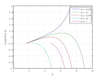
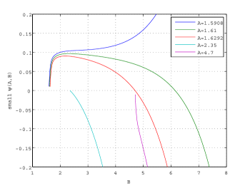
$\Psi(A,B)$	$\psi(A,B)$
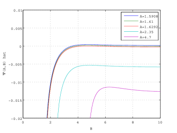
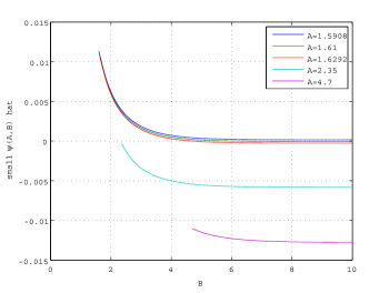
$\widehat{\Psi}(A,B)$	$\widehat{\psi}(A,B)$

Figure 1. Illustration of $\Psi(A,B)$, $\widehat{\Psi}(A,B)$, $\psi(A,B)$, and $\widehat{\psi}(A,B)$ as functions of $B$.

Figure 1 gives numerical plots of $\Psi(A,\cdot)$, $\widehat{\Psi}(A,\cdot)$, $\psi(A,\cdot)$ and $\widehat{\psi}(A,\cdot)$ for various values of $A>0$. Lemma 3.4-(1,2) and the fact that $\widehat{\psi}(A,B)\geq 0\Longleftrightarrow\psi(A,B)\geq 0$ imply that, given a fixed $A$, there are three possible behaviors for $\Psi$:

1. For small $A$, $\Psi(A,B)$ is monotonically increasing in $B$.

2. For large $A$, $\Psi(A,B)$ is monotonically decreasing in $B$.

3. Otherwise $\Psi(A,B)$ first increases and then decreases in $B$.

The behavior of $\Psi$ has implications for the existence and uniqueness of $A^{*}$ and $B^{*}$, as shown in Theorem 3.3 and Lemma 3.5 below. Besides, it can be confirmed that $\widehat{\Psi}(A,\cdot)$ and $\widehat{\psi}(A,\cdot)$ converge as $B\uparrow\infty$ as in Lemmas 3.3-(1) and 3.4-(2). We shall see that the continuous/smooth fit conditions (2.12)-(2.13) require (except for the case $A^{*}=0$ or $B^{*}=\infty$) that $\widehat{\Psi}(A^{*},B^{*})=\widehat{\psi}(A^{*},B^{*})=0$, or equivalently $\Psi(A^{*},B^{*})=\psi(A^{*},B^{*})=0$. This is illustrated by the line corresponding to $A=1.6292$ in Figure 1.

We begin with establishing the continuous fit condition.

Continuous fit at $B$: Continuous fit at $B$ is satisfied automatically for all cases since $v_{A,B}(B-)-h(B)$ exists and

$$v_{A,B}(B-)-h(B)=\Upsilon(B-;A,B)-\Big{(}\frac{\tilde{p}}{r}-\gamma_{b}\Big{)}=0,\quad 0<A<B<\infty,$$ (3.37)

which also holds when $A=0+$ and $v_{0+,B}(B-)-h(B)=0$ given $\int_{0}^{1}u\Pi({\rm d}u)<\infty$. This is also clear from the fact that a spectrally negative Lévy process always creeps upward and hence $B$ is regular for $(B,\infty)$ for any arbitrary level $B>0$ (see [23, p.212]).

Continuous fit at $A$: We examine the limit of $v_{A,B}(x)-g(x)$ as $x\downarrow A$, namely,

$$v_{A,B}(A+)-g(A)=W^{(r)}(0)\widehat{\Psi}(A,B),\quad 0<A<B\leq\infty.$$ (3.38)

In view of (3.14), continuous fit at $A$ holds automatically for the unbounded variation case. For the bounded variation case, the continuous fit condition is equivalent to

$$\widehat{\Psi}(A,B)=0.$$ (3.39)

We now pursue the smooth fit condition. Substituting (3.33) into the derivative of (3.22), we obtain

$$v_{A,B}^{\prime}(x)-h^{\prime}(x)=v_{A,B}^{\prime}(x)-g^{\prime}(x)=\Upsilon^{\prime}(x;A,B)=W^{(r)^{\prime}}(x-A)\widehat{\Psi}(A,B)-\psi(A,x),$$ (3.40)

for every $0<A<x<B\leq\infty$ (extended to $A=0+$ when $\int_{0}^{1}u\Pi({\rm d}u)<\infty$).
Smooth fit at $B$: With (3.40), the smooth fit condition $v_{A,B}^{\prime}(B-)-h^{\prime}(B)=0$ at $B<\infty$ amounts to

$$\frac{\partial}{\partial B}\widehat{\Psi}(A,B)=0$$

because

$$W^{(r)^{\prime}}(B-A)\widehat{\Psi}(A,B)-\psi(A,B)=-W^{(r)}(B-A)\Big{(}\widehat{\psi}(A,B)-\frac{W^{(r)^{\prime}}(B-A)}{W^{(r)}(B-A)}\widehat{\Psi}(A,B)\Big{)}$$

and

$$\frac{\partial}{\partial B}\widehat{\Psi}(A,B)=\widehat{\psi}(A,B)-\frac{W^{(r)^{\prime}}(B-A)}{W^{(r)}(B-A)}\widehat{\Psi}(A,B).$$ (3.41)

For the case $A=0+$ and $\int_{0}^{1}u\Pi({\rm d}u)<\infty$, the smooth fit condition $v_{0+,B}^{\prime}(B-)-h^{\prime}(B)=0$ requires $\frac{\partial}{\partial B}\widehat{\Psi}(0,B)=0$, which is well-defined by Lemmas 3.3-(2) and 3.4-(1) and (3.41).

Smooth fit at $A$: Assuming that it has paths of unbounded variation ($W^{(r)}(0)=0$), then we obtain

$$v_{A,B}^{\prime}(A+)-g^{\prime}(A) =W^{(r)^{\prime}}(0+)\widehat{\Psi}(A,B),\quad 0<A<B\leq\infty.$$

Therefore, (3.39) is also a sufficient condition for smooth fit at $A$ for the unbounded variation case.

We conclude that

1. if $\widehat{\Psi}(A,B)=0$, then continuous fit at $A$ holds for the bounded variation case and both continuous and smooth fit at $A$ holds for the unbounded variation case;

2. if $\frac{\partial}{\partial B}\widehat{\Psi}(A,B)=0$, then both continuous and smooth fit conditions at $B$ hold for all cases.

If both $\widehat{\Psi}(A,B)=0$ and $\frac{\partial}{\partial B}\widehat{\Psi}(A,B)=0$ are satisfied, then $\widehat{\psi}(A,B)=0$ automatically follows by (3.41).

3.4. Existence and Identification of $(A^{*},B^{*})$

In the previous subsection, we have derived the defining equations for the candidate pair $(A^{*},B^{*})$. Nevertheless, the computation of $(A^{*},B^{*})$ is non-trivial and depends on the behaviors of functions $\Psi(A,B)$ and $\psi(A,B)$. In this subsection, we prove the existence of $(A^{*},B^{*})$ and provide a procedure to calculate their values.

Recall from Lemma 3.4-(1) that $\widehat{\psi}(A,\infty)$ is decreasing in $A$ and observe that $\widehat{\psi}(A,A+):=\lim_{x\downarrow A}\widehat{\psi}(A,x)=-(\tilde{p}+r\gamma_{s})+(\tilde{\alpha}-\gamma_{s})\Pi(A,\infty)$ is also decreasing in $A$. Hence, let $\underline{A}$ and $\overline{A}$ be the unique values such that

$$\widehat{\psi}(\underline{A},\infty) \equiv-\left(\tilde{p}+r\gamma_{s}\right)+(\tilde{\alpha}-\gamma_{s})\rho(\underline{A})=0,$$ (3.42)

$$\widehat{\psi}(\overline{A},\overline{A}+) \equiv-\left(\tilde{p}+r\gamma_{s}\right)+(\tilde{\alpha}-\gamma_{s})\Pi(\overline{A},\infty)=0,$$ (3.43)

upon existence; we set the former zero if $\widehat{\psi}(A,\infty)<0$ for all $A\geq 0$ and also set the latter zero if $\widehat{\psi}(A,A+)<0$ for any $A\geq 0$. Since $\rho(A)\downarrow 0$ and $\Pi(A,\infty)\downarrow 0$ as $A\uparrow\infty$, $\overline{A}$ and $\underline{A}$ are finite. In addition, $\rho(A)<\Pi(A,\infty)$ implies that $\overline{A}\geq\underline{A}$.

Define for every $\underline{A}\leq A\leq\overline{A}$,

$$\begin{split}&\underline{b}(A):=\inf\{B>A:\widehat{\Psi}(A,B)\geq 0\}\equiv\inf\left\{B>A:\Psi(A,B)\geq 0\right\},\\ &\overline{b}(A):=\inf\{B>A:\widehat{\psi}(A,B)\leq 0\}\equiv\inf\left\{B>A:\psi(A,B)\leq 0\right\},\\ &b(A):=\inf\{B>A:\widehat{\Psi}(A,B)-\widehat{\psi}(A,B)\frac{W^{(r)}(B-A)}{W^{(r)^{\prime}}(B-A)}\geq 0\},\end{split}$$ (3.44)

where we assume $\inf\emptyset=\infty$. For $b(A)$ above, we recall from (3.41) that

$$\widehat{\Psi}(A,B)-\widehat{\psi}(A,B)\frac{W^{(r)}(B-A)}{W^{(r)^{\prime}}(B-A)}=0\Longleftrightarrow\frac{\partial}{\partial B}\widehat{\Psi}(A,B)=0.$$ (3.45)

Also, using Lemmas 3.3-(1) and 3.4-(2) and that $\Phi(r)\widehat{\Psi}(A,\infty)=\widehat{\psi}(A,\infty)$ (see (3.18), (3.27), and (3.36)), we obtain the limit

$$\lim_{B\uparrow\infty}\Big{(}\widehat{\Psi}(A,B)-\widehat{\psi}(A,B)\frac{W^{(r)}(B-A)}{W^{(r)^{\prime}}(B-A)}\Big{)}=0.$$ (3.46)

Next, we show that there always exists a pair $(A^{*},B^{*})$ belonging to one of the following four cases:

case 1:

$0<A^{*}<B^{*}<\infty$ with $B^{*}=\underline{b}(A^{*})=\overline{b}(A^{*})<\infty$;

case 2:

$0<A^{*}<B^{*}=\infty$ with $B^{*}=\underline{b}(A^{*})=\overline{b}(A^{*})=\infty$ and $\widehat{\Psi}(A^{*},\infty)=0$;

case 3:

$0=A^{*}<B^{*}<\infty$ with $B^{*}=b(0)\leq\underline{b}(0)$;

case 4:

$0=A^{*}<B^{*}=\infty$ with $\underline{b}(0)=\infty$ and $b(0)=\infty$.

Theorem 3.3.

1. If $\underline{A}>0$ and $\underline{b}(\underline{A})<\infty$, then there exists $A^{*}\in(\underline{A},\overline{A})$ such that $B^{*}=\underline{b}(A^{*})=\overline{b}(A^{*})<\infty$. This corresponds to case 1.

2. If $\underline{A}>0$ and $\underline{b}(\underline{A})=\infty$, then $A^{*}=\underline{A}$ and $B^{*}=\infty$ satisfy the condition for case 2.

3. If $\underline{A}=0$, $\overline{A}>0$, and $\underline{b}(0)<\overline{b}(0)$, then there exists $A^{*}\in(0,\overline{A})$ such that $B^{*}=\underline{b}(A^{*})=\overline{b}(A^{*})$. This corresponds to case 1.

4. Suppose (i) $\overline{A}=0$ or (ii) $\underline{A}=0$ and $\underline{b}(0)\geq\overline{b}(0)$. If $b(0)<\infty$, then $A^{*}=0$ and $B^{*}=b(0)$ satisfy the condition for case 3. If $b(0)=\infty$, then $A^{*}=0$ and $B^{*}=\infty$ satisfy the condition for case 4.

In particular, from (3.3) and (3.42) we infer that $\int_{0}^{1}u\Pi({\rm d}u)=\infty$ implies $\underline{A}>0$. This together with Theorem 3.3 leads to the following corollary.

Corollary 3.1.

If $X^{d}$ as in (3.2) has paths of unbounded variation, then $\int_{0}^{1}u\Pi({\rm d}u)=\infty$ and $A^{*}>0$.

Remark 3.5.

Note that $\underline{b}(A)=\overline{b}(A)$ implies $b(A)=\underline{b}(A)=\overline{b}(A)$ (even when they are $+\infty$; see (3.46)). By the construction in (3.44), $A^{*}$ and $B^{*}$ obtained above must satisfy:

1. For every $A^{*}<B<B^{*}$, $\widehat{\Psi}(A^{*},B)<0$ and $\widehat{\Psi}(A^{*},B)-\widehat{\psi}(A^{*},B)\frac{W^{(r)}(B-A^{*})}{W^{(r)^{\prime}}(B-A^{*})}<0$.

2. If $A^{*}>0$, then $\widehat{\Psi}(A^{*},B^{*})=0$  (continuous or smooth fit at $A^{*}$ is satisfied).

3. $\widehat{\Psi}(A^{*},B^{*})-\widehat{\psi}(A^{*},B^{*})\frac{W^{(r)}(B^{*}-A^{*})}{W^{(r)^{\prime}}(B^{*}-A^{*})}=0$  (continuous and smooth fit at $B^{*}$ is satisfied, see (3.45)).

In Theorem 3.3-(1,3), we need to further identify $(A^{*},B^{*})$. To this end, we first observe

Lemma 3.5.

(1)  $\underline{b}(A)$ increases in $A$ on $(\underline{A},\overline{A})$, and (2)  $\overline{b}(A)$ decreases in $A$ on $(\underline{A},\overline{A})$.

This lemma implies that (i) if $\overline{b}(A)>\underline{b}(A)$, then $A^{*}$ must lie on $(A,\overline{A})$ and (ii) if $\overline{b}(A)<\underline{b}(A)$, then $A^{*}$ must lie on $(\underline{A},A)$. By Lemma 3.5 and Theorem 3.3, the following algorithm, motivated by the bisection method, is guaranteed to output the pair $(A^{*},B^{*})$. Here let $\varepsilon>0$ be the error parameter.

Step 1:

Compute $\underline{A}$ and $\overline{A}$.

Step 1-1:

If (i) $\overline{A}=0$ or (ii) $\underline{A}=0$ and $\underline{b}(0)\geq\overline{b}(0)$, then stop and conclude that this is case 3 or 4 with $A^{*}=0$ and $B^{*}=b(0)$.

Step 1-2:

If $\underline{A}>0$ and $\underline{b}(\underline{A})=\infty$, then stop and conclude that this is case 2 with $A^{*}=\underline{A}$ and $B^{*}=\infty$.

Step 2:

Set $A=(\underline{A}+\overline{A})/2$.

Step 3:

Compute $\overline{b}(A)$ and $\underline{b}(A)$.

Step 3-1:

If $|\overline{b}(A)-\underline{b}(A)|\leq\varepsilon$, then stop and conclude that this is case 1 with $A^{*}=A$ and $B^{*}=\underline{b}(A)$ (or $B^{*}=\overline{b}(A)$).

Step 3-2:

If $|\overline{b}(A)-\underline{b}(A)|>\varepsilon$ and $\overline{b}(A)>\underline{b}(A)$, then set $\underline{A}=A$ and go back to Step 2.

Step 3-3:

If $|\overline{b}(A)-\underline{b}(A)|>\varepsilon$ and $\overline{b}(A)<\underline{b}(A)$, then set $\overline{A}=A$ and go back to Step 2.

3.5. Verification of Equilibrium

We are now ready to prove Theorems 3.1-3.2. Our candidate value function for the Nash equilibrium is given by (2.11) and (3.19) with $A^{*}$ and $B^{*}$ obtained by the procedure above. By Lemma 3.1,

$$\begin{split}v_{A^{*},B^{*}}(x)&=\left\{\begin{array}[]{ll}h(x),&x\geq B^{*}\\ h(x)+(v_{A^{*},B^{*}}(x)-h(x)),&A^{*}<x<B^{*}\\ g(x),&x\leq A^{*}\end{array}\right\}=-\Big{(}\frac{\tilde{p}}{r}+\tilde{\alpha}\Big{)}\zeta(x)+J(x)\end{split}$$ (3.47)

where

$$J(x):=\left\{\begin{array}[]{ll}\frac{\tilde{p}}{r}-\gamma_{b},&x\geq B^{*},\\ \Upsilon(x;A^{*},B^{*}),&A^{*}<x<B^{*},\\ \frac{\tilde{p}}{r}+\gamma_{s},&0<x\leq A^{*},\\ \frac{\tilde{p}}{r}+\tilde{\alpha}&x\leq 0.\end{array}\right.$$ (3.52)

When $A^{*}>0$, $(\sigma_{A^{*}},\tau_{B^{*}})$ is the candidate saddle point that attains $v_{A^{*},B^{*}}(x)$. When $A^{*}=0$, $v_{0+,B^{*}}(x)$ can be approximated by $(\sigma_{\varepsilon},\tau_{B^{*}})$ for sufficiently small $\varepsilon>0$. The value of $\Upsilon(x;A^{*},B^{*})$ can be computed by (3.22), (3.30) and (3.31).

The proof of Theorems 3.1-3.2 involves the crucial steps:

1. Domination property

   1. $\mathbb{E}^{x}\left[e^{-r(\tau\wedge\sigma_{A^{*}})}v_{A^{*},B^{*}}(X_{\tau\wedge\sigma_{A^{*}}})1_{\{\tau\wedge\sigma_{A^{*}}<\infty\}}\right]\geq v(x;\sigma_{A^{*}},\tau)$ for all $\tau\in\mathcal{S}$;

   2. $\mathbb{E}^{x}\left[e^{-r(\sigma\wedge\tau_{B^{*}})}v_{A^{*},B^{*}}(X_{\sigma\wedge\tau_{B^{*}}})1_{\{\sigma\wedge\tau_{B^{*}}<\infty\}}\right]\leq v(x;\sigma,\tau_{B^{*}})$ for all $\sigma\in\mathcal{S}$;

2. Sub/super-harmonic property

   1. $(\mathcal{L}-r)v_{A^{*},B^{*}}(x)>0$ for every $0<x<A^{*}$;

   2. $(\mathcal{L}-r)v_{A^{*},B^{*}}(x)=0$ for every $A^{*}<x<B^{*}$;

   3. $(\mathcal{L}-r)v_{A^{*},B^{*}}(x)<0$ for every $x>B^{*}$.

Here $\mathcal{L}$ is the infinitesimal generator associated with the process $X$

$$\mathcal{L}f(x) =cf^{\prime}(x)+\frac{1}{2}\nu^{2}f^{\prime\prime}(x)+\int_{0}^{\infty}\left[f(x-z)-f(x)+f^{\prime}(x)z1_{\{0<z<1\}}\right]\Pi({\rm d}z)$$

applied to any bounded and sufficiently smooth function $f$ that is $C^{2}$ when $X$ is of unbounded variation and $C^{1}$ otherwise.

After establishing (i)-(ii) above, we will apply them to establish (2.10) by showing for the candidate optimal thresholds $(A^{*},B^{*})$ that

$$v(x;\sigma_{A^{*}},\tau)\leq v_{A^{*},B^{*}}(x)\leq v(x;\sigma,\tau_{B^{*}}),\qquad\forall\sigma,\tau\in\mathcal{S}.$$ (3.53)

Remark 3.6.

In fact, it is sufficient to show (3.53) holds for all $\tau\in\mathcal{S}_{A^{*}}$ and $\sigma\in\mathcal{S}_{B^{*}}$, where

$$\begin{split}\mathcal{S}_{A^{*}}:=\left\{\tau\in\mathcal{S}:X_{\tau}\notin(0,A^{*}]\;a.s.\right\}\quad\textrm{and}\quad\mathcal{S}_{B^{*}}:=\left\{\sigma\in\mathcal{S}:X_{\sigma}\notin[B^{*},\infty)\;a.s.\right\}.\end{split}$$ (3.54)

Indeed, for any candidate $\tau\in\mathcal{S}$, it follows that $v(x;\sigma_{A^{*}},\tau)\leq v(x;\sigma_{A^{*}},\hat{\tau})$ where $\hat{\tau}:=\tau 1_{\{X_{\tau}\notin(0,A^{*}]\}}+{\sigma_{0}}1_{\{X_{\tau}\in(0,A^{*}]\}}\in\mathcal{S}_{A^{*}}$, so the buyer’s optimal exercise time $\tau^{*}$ must belong to $\mathcal{S}_{A^{*}}$. This is intuitive since the seller will end the game as soon as $X$ enters $(0,A^{*}]$ and hence the buyer should not needlessly stop in this interval and pay $\gamma_{b}$. Similar arguments apply to the use of $\mathcal{S}_{B^{*}}$. Then, using the same arguments as for (2.11), we can again safely eliminate the $f(\cdot)$ term in (2.6) and write

$$v(x;\sigma_{A^{*}},\tau) =\mathbb{E}^{x}\left[e^{-r(\tau\wedge\sigma_{A^{*}})}\left(h(X_{\tau})1_{\{\tau<\sigma_{A^{*}}\}}+g(X_{\sigma_{A^{*}}})1_{\{\tau>\sigma_{A^{*}}\}}\right)1_{\{\tau\wedge\sigma_{A^{*}}<\infty\}}\right],\quad\tau\in\mathcal{S}_{A^{*}},$$

$$v(x;\sigma,\tau_{B^{*}}) =\mathbb{E}^{x}\left[e^{-r(\tau_{B^{*}}\wedge\sigma)}\left(h(X_{\tau_{B^{*}}})1_{\{\tau_{B^{*}}<\sigma\}}+g(X_{\sigma})1_{\{\tau_{B^{*}}>\sigma\}}\right)1_{\{\tau_{B^{*}}\wedge\sigma<\infty\}}\right],\quad\sigma\in\mathcal{S}_{B^{*}}.$$

We prove properties (i)-(ii) above using the following lemmas.

Lemma 3.6.

For every $x\in(A^{*},B^{*})$, the following inequalities hold:

$$v_{A^{*},B^{*}}(x)-g(x) \leq 0,$$ (3.55)

$$v_{A^{*},B^{*}}(x)-h(x) \geq 0,$$ (3.56)

where it is understood for the case $A^{*}=0$ and $\nu>0$ that the above results hold with $A^{*}=0+$.

Applying this lemma and the definitions of $\mathcal{S}_{A^{*}}$ and $\mathcal{S}_{B^{*}}$ in (3.54) of Remark 3.6, we obtain

Lemma 3.7.

Fix $x>0$.

1. For every $\tau\in\mathcal{S}_{A^{*}}$, when $A^{*}>0$

   $$g(X_{\sigma_{A^{*}}})1_{\{\sigma_{A^{*}}<\tau\}}+h(X_{\tau})1_{\{\tau<\sigma_{A^{*}}\}}\leq v_{A^{*},B^{*}}(X_{\sigma_{A^{*}}\wedge\tau}),\quad\mathbb{P}^{x}\textrm{-a.s.}\;\textrm{on }\{\sigma_{A^{*}}\wedge\tau<\infty\},$$

   and when $A^{*}=0$,

   $$-(\tilde{\alpha}-\gamma_{s})1_{\{X_{\tau}=0\}}+h(X_{\tau})1_{\{\tau<{\sigma_{0}}\}}\leq v_{0+,B^{*}}(X_{\tau}),\quad\mathbb{P}^{x}\textrm{-a.s.}\;\textrm{on }\{\tau<\infty\}.$$

2. For every $\sigma\in\mathcal{S}_{B^{*}}$,

   $$g(X_{\sigma})1_{\{\sigma<\tau_{B^{*}}\}}+h(X_{\tau_{B^{*}}})1_{\{\tau_{B^{*}}<\sigma\}}\geq v_{A^{*},B^{*}}(X_{\sigma\wedge\tau_{B^{*}}}),\quad\mathbb{P}^{x}\textrm{-a.s.}\;\textrm{on }\{\sigma\wedge\tau_{B^{*}}<\infty\},$$

   where it is understood for the case $A^{*}=0$ and $\nu>0$ that the above holds with $A^{*}=0+$.

Lemma 3.8.

1. When $A^{*}>0$, we have $(\mathcal{L}-r)v_{A^{*},B^{*}}(x)>0$ for every $0<x<A^{*}$.

2. We have $(\mathcal{L}-r)v_{A^{*},B^{*}}(x)=0$ for every $A^{*}<x<B^{*}$.

3. When $B^{*}<\infty$, we have $(\mathcal{L}-r)v_{A^{*},B^{*}}(x)<0$ for every $x>B^{*}$.

The domination property (i) holds by applying discounting and expectation in Lemma 3.7. The sub/super-harmonic property (ii) is implied by Lemma 3.8. By Ito’s lemma, this shows that the stopped processes $e^{-r(t\wedge\sigma_{A^{*}})}v_{A^{*},B^{*}}(X_{t\wedge\sigma_{A^{*}}})$ and $e^{-r(t\wedge\tau_{B^{*}})}v_{A^{*},B^{*}}(X_{t\wedge\tau_{B^{*}}})$ are, respectively, a supermartingale and a submartingale. In turn, we apply them to show $v_{A^{*},B^{*}}(x)\geq v(x;\sigma_{A^{*}},\tau)$ for any arbitrary $\tau\in\mathcal{S}_{A^{*}}$, and $v_{A^{*},B^{*}}(x)\leq v(x;\sigma,\tau_{B^{*}})$ for any arbitrary $\sigma\in\mathcal{S}_{B^{*}}$, that is, the Nash equilibrium. We provide the details of the proofs for Theorems 3.1-3.2 in the Appendix.

4. Exponential Jumps and Numerical Examples

In this section, we consider spectrally negative Lévy processes with i.i.d. exponential jumps and provide some numerical examples to illustrate the buyer’s and seller’s optimal exercise strategies and the impact of step-up/down fees on the game value. The results obtained here can be extended easily to the hyperexponential case using the explicit expression of the scale function obtained by [15], and can be used to approximate for a general case with a completely monotone density (see, e.g., [15, 18]). Here, however, we focus on a rather simple case for more intuitive interpretation of our numerical results.

4.1. Spectrally Negative Lévy Processes with Exponential Jumps

Let $X$ be a spectrally negative Lévy process of the form

$$X_{t}-X_{0}=\mu t+\nu B_{t}-\sum_{n=1}^{N_{t}}Z_{n},\quad 0\leq t<\infty.$$

Here $B=\{B_{t};t\geq 0\}$ is a standard Brownian motion, $N=\{N_{t};t\geq 0\}$ is a Poisson process with arrival rate $\lambda$, and $Z=\left\{Z_{n};n=1,2,\ldots\right\}$ is an i.i.d. sequence of exponential random variables with density function $f(z):=\eta e^{-\eta z}$, $z>0$, for some $0<\eta<\infty$. Its Laplace exponent (3.1) is given by

$$\phi(s)=\mu s+\frac{1}{2}\nu^{2}s^{2}-\lambda\frac{s}{\eta+s}.$$

For our examples, we assume $\nu>0$. In this case, there are two negative solutions to the equation $\phi(s)=r$ and their absolute values $\{\xi_{i,r};i=1,2\}$ satisfy the interlacing condition: $0<\xi_{1,r}<\eta<\xi_{2,r}<\infty$. For this process, the scale function is given by for every $x\geq 0$

$$\begin{split}W^{(r)}(x)&=\sum_{i=1}^{2}C_{i}\left[e^{\Phi(r)x}-e^{-\xi_{i,r}x}\right],\end{split}$$ (4.1)

for some $C_{1}$ and $C_{2}$ (see [15] for their expressions). In addition, applying (4.1) to (3.7) yields

$$W_{\Phi(r)}(x) =\sum_{i=1}^{2}C_{i}\left[1-e^{-(\Phi(r)+\xi_{i,r})x}\right],$$

with the limit $W_{\Phi(r)}(\infty)=\sum_{i=1}^{2}C_{i}$, which equals $(\phi^{\prime}(\Phi(r)))^{-1}$ by (3.8).

Recall that, in contrast to $\psi(A,B)$ and $\Psi(A,B)$, $\widehat{\psi}(A,B)$ and $\widehat{\Psi}(A,B)$ do not explode. Therefore, they are used to compute the optimal thresholds $A^{*}$ and $B^{*}$ and the value function $V$. Below we provide the formulas for $\widehat{\psi}(A,B)$ and $\widehat{\Psi}(A,B)$. The computations are very tedious but straightforward, so we omit the proofs here.

In summary, for $B>A\geq 0$, we have

$$\widehat{\psi}(A,B)=-\left(\tilde{p}+\gamma_{s}r\right)+\left(\tilde{\alpha}-\gamma_{s}\right)\lambda e^{-\eta A}-\frac{W_{\Phi(r)}(\infty)}{W_{\Phi(r)}(B-A)}(\tilde{\alpha}-\gamma_{s})\lambda\frac{\eta}{\Phi(r)+\eta}e^{-\eta A}\\ +\frac{\tilde{\alpha}-\gamma_{s}}{W_{\Phi(r)}(B-A)}\lambda e^{-\Phi(r)(B-A)}\sum_{i=1}^{2}C_{i}\Big{[}\frac{\eta}{\Phi(r)+\eta}e^{-\eta B}+\frac{\eta}{\xi_{i,r}-\eta}\left(e^{-\eta B}-e^{-\xi_{i,r}(B-A)-\eta A}\right)\Big{]}$$

and

$$\widehat{\Psi}(A,B)=\frac{1}{W_{\Phi(r)}(B-A)}\Big{[}W_{\Phi(r)}(\infty)\Big{(}\lambda e^{-\eta A}\frac{\tilde{\alpha}-\gamma_{s}}{\Phi(r)+\eta}-\frac{\tilde{p}+\gamma_{s}r}{\Phi(r)}\Big{)}+{e^{-\Phi(r)(B-A)}}\varrho(A,B)\Big{]}$$

where

$$\varrho(A,B):=\left(\tilde{\alpha}-\gamma_{s}\right)\lambda\sum_{i=1}^{2}C_{i}\Big{(}e^{-\eta B}\Big{[}-\frac{1}{\Phi(r)+\eta}+\frac{1}{\xi_{i,r}-\eta}\Big{]}-e^{-\eta A-\xi_{i,r}(B-A)}\frac{1}{\xi_{i,r}-\eta}\Big{)}\\ -\left(\tilde{p}+\gamma_{s}r\right)\sum_{i=1}^{2}C_{i}\Big{[}-\frac{1}{\Phi(r)}+\frac{1}{\xi_{i,r}}\left(e^{-\xi_{i,r}(B-A)}-1\right)\Big{]}-\left(\gamma_{b}+\gamma_{s}\right).$$

Also, setting $B=\infty$ and $B=A+$, (3.42)-(3.43) yield

$$\widehat{\psi}(A,\infty)=-\left(\tilde{p}+\gamma_{s}r\right)+\lambda(\tilde{\alpha}-\gamma_{s})\frac{\Phi(r)}{\Phi(r)+\eta}e^{-\eta A}\quad\textrm{and}\quad\widehat{\psi}(A,A+)=-\left(\tilde{p}+\gamma_{s}r\right)+\left(\tilde{\alpha}-\gamma_{s}\right)\lambda e^{-\eta A}.$$

4.2. Numerical Results

Let us denote the step-up/down ratio by $q:=\hat{p}/p=\hat{\alpha}/\alpha.$ We consider four contract specifications:

1. cancellation game with $q=0$   (position canceled at exercise),

2. step-down game with $q=0.5$   (position halved at exercise),

3. vanilla CDS with $q=1.0$   (position unchanged at exercise),

4. step-up game with $q=1.5$   (position raised at exercise).

The model parameters are $r=0.03$, $\lambda=1.0$, $\eta=2.0$, $\nu=0.2$, $\alpha=1$, $x=1.5$ and $\gamma_{s}=\gamma_{b}=1000$ bps, unless specified otherwise. We also choose $\mu$ so that the risk-neutral condition $\phi(1)=r$ is satisfied.

Figure 2 shows for all four cases the contract value $V$ to the buyer as a function of $x$ given a fixed premium rate. It is decreasing in $x$ since default is less likely for higher value of $x$. For the cancellation game, $V$ takes the constant values $\gamma_{s}=1000$ bps for $x\leq A^{*}$ and $-\gamma_{b}=-1000$ bps for $x\geq B^{*}$ since in these regions immediate cancellation with a fee is optimal.

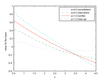
Figure 2. The value for the buyer $V(x;\sigma_{A^{*}},\tau_{B^{*}})$ as a function of $x$. Here $r=0.03$, $p=0.05$, $\mu=0.1352$, $\lambda=1.0$, $\eta=2.0$, $\nu=0.2$, and $\gamma_{b}=\gamma_{s}=1000$ bps.

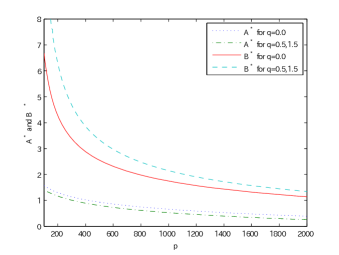
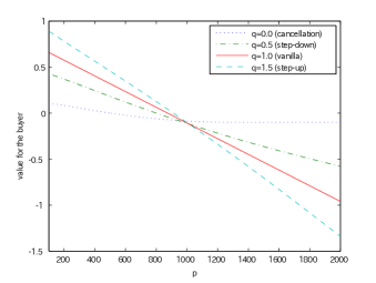
Figure 3. (Left) Optimal threshold levels $A^{*}$ and $B^{*}$ and (right) the value for the buyer with respect to $p$. The parameters are $r=0.03$, $x=1.5$, $\mu=0.3433$, $\lambda=0.5$, $\eta=2.0$, $\nu=0.2$, and $\gamma_{b}=\gamma_{s}=1000$ bps.

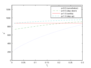
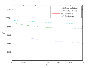
Figure 4. The equilibrium premium $p^{*}$ with respect to $\gamma_{s}$ (left) and $\gamma_{b}$ (right). Here $r=0.03$, $x=1.5$, $\mu=0.3433$, $\lambda=1.0$, $\eta=2.0$, $\nu=0.2$, and $\gamma_{b}=\gamma_{s}=1000$ bps unless specified otherwise.

In Figure 3, we show the optimal thresholds $A^{*}$ and $B^{*}$ and the value $V$ with respect to $p$. The symmetry argument discussed in Section 2 applies to the cases (D) and (U). As a result, the $A^{*}$ in (D) is identical to the $B^{*}$ in (U), and the $B^{*}$ in (D) is identical to the $A^{*}$ in (U). In all four cases, both $A^{*}$ and $B^{*}$ are decreasing in $p$. In other words, as $p$ increases, the buyer tends to exercise earlier while the seller tends to delay exercise. Intuitively, a higher premium makes waiting more costly for the buyer but more profitable for the seller. The value $V$ in the cancellation game stays constant when $p$ is sufficiently small because the seller would exercise immediately; it also becomes flat when $p$ is sufficiently high because the buyer would exercise immediately.

Note that the value function $V$ and the optimal stopping strategies $(\sigma^{*},\tau^{*})$ depend on the premium rate $p$. In particular, we call $p^{*}$ the equilibrium premium rate if it yields $V(x;\sigma^{*}(p^{*}),\tau^{*}(p^{*}))=0$, where we emphasize the saddle point $(\sigma^{*}(p^{*}),\tau^{*}(p^{*}))$ corresponds to $p^{*}$. Hence, under the equilibrium premium rate, the default swap game starts at value zero, implying no cash transaction between the protection buyer and seller at contract initiation. As illustrated in Figure 3-(b), the value $V$ (from the buyer’s perspective) is always decreasing in $p$. Using a bisection method, we numerically determine the equilibrium premium $p^{*}$ so that $V=0$. We illustrate in Figure 4 the equilibrium premium $p^{*}$ as a function of $\gamma_{b}$ and $\gamma_{s}$. As is intuitive, the equilibrium premium $p^{*}$ is increasing in $\gamma_{s}$ and decreasing in $\gamma_{b}$.

5. Conclusions

We have discussed the valuation of a default swap contract where the protection buyer and seller can alter the respective position once prior to default. This new contractual feature drives the protection buyer/seller to consider the optimal timing to control credit risk exposure. The valuation problem involves the analytical and numerical studies of an optimal stopping game with early termination from default. Under a perpetual setting, the investors’ optimal stopping rules are characterized by their respective exercise thresholds, which can be quickly determined in a general class of spectrally negative Lévy credit risk models.

For future research, it is most natural to consider the default swap game under a finite horizon and/or different credit risk models. The default swap game studied in this paper can potentially be applied to approximate its finite-maturity version using the maturity randomization (Canadization) approach (see [11, 25]). Another interesting extension is to allow for multiple adjustments by the buyer and/or seller prior to default, which can be modeled as stochastic games with multiple stopping opportunities. Finally, the step-up and step-down features also arise in other derivatives, including interest rate swaps.

Appendix A Proofs

Proof of Proposition 2.1.

First, by a rearrangement of integrals and (2.5), the expression inside the expectation in (2.1) can be written as

$$1_{\{\tau\wedge\sigma<\infty\}}\Big{[}\int_{\tau\wedge\sigma}^{\sigma_{0}}e^{-rt}\tilde{p}\,{\rm d}t-\int_{0}^{\sigma_{0}}e^{-rt}p\,{\rm d}t+e^{-r{\sigma_{0}}}\left(-\tilde{\alpha}1_{\{\tau\wedge\sigma<{\sigma_{0}}\}}+\alpha\right)$$

$$\qquad+1_{\{\tau\wedge\sigma<{\sigma_{0}}\}}e^{-r(\tau\wedge\sigma)}\left(-\gamma_{b}1_{\{\tau\leq\sigma\}}+\gamma_{s}1_{\{\tau\geq\sigma\}}\right)\Big{]}+1_{\{\tau\wedge\sigma=\infty\}}\Big{(}-\int_{0}^{\infty}e^{-rt}p\,{\rm d}t\Big{)}$$

$$=1_{\{\tau\wedge\sigma<\infty\}}\Big{(}\int_{\tau\wedge\sigma}^{\sigma_{0}}e^{-rt}\tilde{p}\,{\rm d}t-e^{-r{\sigma_{0}}}\tilde{\alpha}1_{\{\tau\wedge\sigma<{\sigma_{0}}\}}+1_{\{\tau\wedge\sigma<{\sigma_{0}}\}}e^{-r(\tau\wedge\sigma)}\left(-\gamma_{b}1_{\{\tau\leq\sigma\}}+\gamma_{s}1_{\{\tau\geq\sigma\}}\right)\Big{)}$$

$$-\int_{0}^{{\sigma_{0}}}e^{-rt}p\,{\rm d}t+e^{-r{\sigma_{0}}}\alpha$$

$$=1_{\{\tau\wedge\sigma<\infty,\;\tau\wedge\sigma<{\sigma_{0}}\}}\Big{(}\int_{\tau\wedge\sigma}^{\sigma_{0}}e^{-rt}\tilde{p}\,{\rm d}t-e^{-r{\sigma_{0}}}\tilde{\alpha}+e^{-r(\tau\wedge\sigma)}\left(-\gamma_{b}1_{\{\tau\leq\sigma\}}+\gamma_{s}1_{\{\tau\geq\sigma\}}\right)\Big{)}-\int_{0}^{{\sigma_{0}}}e^{-rt}p\,{\rm d}t+e^{-r{\sigma_{0}}}\alpha.$$

Taking expectation, (2.1) simplifies to

$$V(x;\sigma,\tau) =\mathbb{E}^{x}\Big{[}1_{\{\tau\wedge\sigma<\infty,\;\tau\wedge\sigma<{\sigma_{0}}\}}\Big{(}\int_{\tau\wedge\sigma}^{\sigma_{0}}e^{-rt}\tilde{p}\,{\rm d}t-e^{-r{\sigma_{0}}}\tilde{\alpha}+e^{-r(\tau\wedge\sigma)}\left(-\gamma_{b}1_{\{\tau\leq\sigma\}}+\gamma_{s}1_{\{\tau\geq\sigma\}}\right)\Big{)}\Big{]}$$ (A.1)

$$-\mathbb{E}^{x}\Big{[}\int_{0}^{\sigma_{0}}e^{-rt}p\,{\rm d}t\Big{]}+\alpha\,\mathbb{E}^{x}\left[e^{-r{\sigma_{0}}}\right].$$

Here, the last two terms do not depend on $\tau$ nor $\sigma$ and they constitute $C(x;p,\alpha)$. Next, using the fact that $\{\tau\wedge\sigma<{\sigma_{0}},\tau\wedge\sigma<\infty\}=\{X_{\tau\wedge\sigma}>0,\;\tau\wedge\sigma<\infty\}$ for every $\tau,\sigma\in\mathcal{S}$ and the strong Markov property of $X$ at time $\tau\wedge\sigma$, we express the first term as

$$\mathbb{E}^{x}\Big{[}1_{\{\tau\wedge\sigma<\infty,\;\tau\wedge\sigma<{\sigma_{0}}\}}\Big{(}\mathbb{E}^{x}\Big{[}\int_{\tau\wedge\sigma}^{\sigma_{0}}e^{-rt}\tilde{p}\,{\rm d}t-e^{-r{\sigma_{0}}}\tilde{\alpha}\Big{|}\mathcal{F}_{\tau\wedge\sigma}\Big{]}+e^{-r(\tau\wedge\sigma)}\left(-\gamma_{b}1_{\{\tau\leq\sigma\}}+\gamma_{s}1_{\{\tau\geq\sigma\}}\right)\Big{)}\Big{]}$$

$$=\mathbb{E}^{x}\left[1_{\{\tau\wedge\sigma<\infty,\;\tau\wedge\sigma<{\sigma_{0}}\}}e^{-r(\tau\wedge\sigma)}\left(h(X_{\tau})1_{\{\tau<\sigma\}}+g(X_{\sigma})1_{\{\tau>\sigma\}}+f(X_{\tau})1_{\{\tau=\sigma\}}\right)\right]$$

$$=\mathbb{E}^{x}\left[e^{-r(\tau\wedge\sigma)}\left(h(X_{\tau})1_{\{\tau<\sigma\}}+g(X_{\sigma})1_{\{\tau>\sigma\}}+f(X_{\tau})1_{\{\tau=\sigma\}}\right)1_{\{\tau\wedge\sigma<\infty\}}\right]=v(x;\sigma,\tau),$$

where the second equality holds because (i) $\tau<\sigma$ or $\tau>\sigma$ implies $\tau\wedge\sigma<{\sigma_{0}}$, and (ii) by $f(X_{\sigma_{0}})=0$ we have $f(X_{\tau})1_{\{\tau=\sigma,\tau\wedge\sigma<{\sigma_{0}}\}}=f(X_{\tau})1_{\{\tau=\sigma\}}$ a.s. ∎

Proof of Proposition 2.2.

First, we deduce from (2.7)-(2.9) that

$$h(x;\tilde{p},\tilde{\alpha},\gamma_{b}) =-g(x;-\tilde{p},-\tilde{\alpha},\gamma_{b}),$$

$$g(x;\tilde{p},\tilde{\alpha},\gamma_{s}) =-h(x;-\tilde{p},-\tilde{\alpha},\gamma_{s}),$$

$$f(x;\tilde{p},\tilde{\alpha},\gamma_{b},\gamma_{s}) =-f(x;-\tilde{p},-\tilde{\alpha},\gamma_{s},\gamma_{b}).$$

Substituting these equations to (2.6) of Proposition 2.1, it follows, for every $\tau,\sigma\in\mathcal{S}$, that

$$v(x;\sigma,\tau;\tilde{p},\tilde{\alpha},\gamma_{b},\gamma_{s}) =-\mathbb{E}^{x}\left[e^{-r(\tau\wedge\sigma)}\left(h(X_{\sigma};-\tilde{p},-\tilde{\alpha},\gamma_{s})1_{\{\sigma<\tau\}}+g(X_{\tau};-\tilde{p},-\tilde{\alpha},\gamma_{b})1_{\{\tau<\sigma\}}\right.\right.$$

$$\qquad\left.\left.+f(X_{\tau\wedge\sigma};-\tilde{p},-\tilde{\alpha},\gamma_{s},\gamma_{b})1_{\{\tau=\sigma\}}\right)1_{\{\tau\wedge\sigma<\infty\}}\right]$$

$$=-v(x;\tau,\sigma;-\tilde{p},-\tilde{\alpha},\gamma_{s},\gamma_{b}).$$

∎

Proof of Lemma 3.1.

Recall that $v$ is given by the first expectation of (A.1), and note that $\sigma_{A}\wedge\tau_{B}=\infty$ implies ${\sigma_{0}}=\infty$. For every $x\in(A,B)$, $v(x;A,B)-h(x)$ equals

$$\mathbb{E}^{x}\Big{[}1_{\{\sigma_{A}\wedge\tau_{B}<\infty\}}\Big{(}\int_{\sigma_{A}\wedge\tau_{B}}^{{\sigma_{0}}}e^{-rt}\tilde{p}\,{\rm d}t-e^{-r{\sigma_{0}}}\tilde{\alpha}1_{\{\sigma_{A}\wedge\tau_{B}<{\sigma_{0}}\}}+e^{-r(\sigma_{A}\wedge\tau_{B})}\left(-\gamma_{b}1_{\{\tau_{B}<\sigma_{A}\}}+\gamma_{s}1_{\{\tau_{B}>\sigma_{A}\}}\right)\Big{)}\Big{]}$$

$$\qquad-\mathbb{E}^{x}\Big{[}\int_{0}^{\sigma_{0}}e^{-rt}\tilde{p}\,{\rm d}t\,-e^{-r{\sigma_{0}}}\tilde{\alpha}\,\Big{]}+\gamma_{b}$$

$$=\mathbb{E}^{x}\Big{[}1_{\{\sigma_{A}\wedge\tau_{B}<\infty\}}\Big{(}-\int_{0}^{\sigma_{A}\wedge\tau_{B}}e^{-rt}\tilde{p}\,{\rm d}t+e^{-r{\sigma_{0}}}\tilde{\alpha}1_{\{\sigma_{A}\wedge\tau_{B}={\sigma_{0}}\}}+e^{-r(\sigma_{A}\wedge\tau_{B})}\left(-\gamma_{b}1_{\{\tau_{B}<\sigma_{A}\}}+\gamma_{s}1_{\{\tau_{B}>\sigma_{A}\}}\right)\Big{)}$$

$$\qquad-1_{\{\sigma_{A}\wedge\tau_{B}=\infty\}}\Big{(}\int_{0}^{\sigma_{0}}e^{-rt}\tilde{p}\,{\rm d}t\,-e^{-r{\sigma_{0}}}\tilde{\alpha}\Big{)}\,\Big{]}+\gamma_{b}$$

$$=\mathbb{E}^{x}\Big{[}1_{\{\sigma_{A}\wedge\tau_{B}<\infty\}}e^{-r(\sigma_{A}\wedge\tau_{B})}\left(\tilde{\alpha}1_{\{\sigma_{A}\wedge\tau_{B}={\sigma_{0}}\}}-\gamma_{b}1_{\{\tau_{B}<\sigma_{A}\}}+\gamma_{s}1_{\{\tau_{B}>\sigma_{A}\}}\right)-\int_{0}^{\sigma_{A}\wedge\tau_{B}}e^{-rt}\tilde{p}\,{\rm d}t\,\Big{]}+\gamma_{b},$$

which equals $\Upsilon(x;A,B)-\frac{\tilde{p}}{r}+\gamma_{b}$. Since $g(x)=h(x)+\gamma_{s}+\gamma_{b}$, $\forall x>0$, the second claim of (3.21) is immediate.

The proof of the second claim amounts to proving the following: for $0<A<x<B<\infty$,

$$\begin{split}\mathbb{E}^{x}\left[e^{-r(\sigma_{A}\wedge\tau_{B})}1_{\{\tau_{B}<\sigma_{A}\}}\right]&=\frac{W^{(r)}(x-A)}{W^{(r)}(B-A)},\\ \mathbb{E}^{x}\left[e^{-r(\sigma_{A}\wedge\tau_{B})}1_{\{\tau_{B}>\sigma_{A}\,\textrm{or}\;\sigma_{A}\wedge\tau_{B}={\sigma_{0}}\}}\right]&=Z^{(r)}(x-A)-Z^{(r)}(B-A)\frac{W^{(r)}(x-A)}{W^{(r)}(B-A)},\\ \mathbb{E}^{x}\left[e^{-r(\sigma_{A}\wedge\tau_{B})}1_{\{\sigma_{A}\wedge\tau_{B}={\sigma_{0}}\}}\right]&=\frac{W^{(r)}(x-A)}{W^{(r)}(B-A)}\kappa(B;A)-\kappa(x;A).\end{split}$$ (A.2)

The first two equalities follow directly from the property of the scale function (see, for example, Theorem 8.1 of [23]). Notice here that $\tau_{B}<\sigma_{A}$ if and only if it up-crosses $B$ before down-crossing $A$ while $\tau_{B}>\sigma_{A}$ or $\sigma_{A}\wedge\tau_{B}={\sigma_{0}}$ if and only if it down-crosses $A$ before up-crossing $B$.

For the third equality, we require the overshoot distribution that is again obtained via the scale function. Let $N$ be the Poisson random measure for the jumps of $-X$ and $\overline{X}$ and $\underline{X}$ be the running maximum and minimum, respectively, of $X$. By compensation formula (see e.g. Theorem 4.4 of [23]), we have

$$\begin{split}\mathbb{E}^{x}\left[e^{-r(\sigma_{A}\wedge\tau_{B})}1_{\{\sigma_{A}\wedge\tau_{B}={\sigma_{0}}\}}\right]&=\mathbb{E}^{x}\Big{[}\int_{0}^{\infty}\int_{0}^{\infty}N({\rm d}t\times{\rm d}u)e^{-rt}1_{\{\overline{X}_{t-}<B,\;\underline{X}_{t-}>A,\;X_{t-}-u<0\}}\Big{]}\\ &=\mathbb{E}^{x}\Big{[}\int_{0}^{\infty}{\rm d}te^{-rt}\int_{0}^{\infty}\Pi({\rm d}u)1_{\{\overline{X}_{t-}<B,\;\underline{X}_{t-}>A,\;X_{t-}-u<0\}}\Big{]}\\ &=\int_{0}^{\infty}\Pi({\rm d}u)\int_{0}^{\infty}{\rm d}t\left[e^{-rt}\mathbb{P}^{x}\{X_{t-}<u,\sigma_{A}\wedge\tau_{B}\geq t\}\right].\end{split}$$ (A.3)

Recall that, as in Theorem 8.7 of [23], the resolvent measure for the spectrally negative Lévy process killed upon exiting $[0,a]$ is given by

$$\int_{0}^{\infty}{\rm d}t\left[e^{-rt}\mathbb{P}^{x}\left\{X_{t-}\in{\rm d}y,\sigma_{0}\wedge\tau_{a}>t\right\}\right]={\rm d}y\left[\frac{W^{(r)}(x)W^{(r)}(a-y)}{W^{(r)}(a)}-W^{(r)}(x-y)\right],\quad y>0.$$

Hence

$$\int_{0}^{\infty}{\rm d}t\left[e^{-rt}\mathbb{P}^{x}\left\{X_{t-}\in{\rm d}y,\sigma_{A}\wedge\tau_{B}>t\right\}\right] =\int_{0}^{\infty}{\rm d}t\left[e^{-rt}\mathbb{P}^{x-A}\left\{X_{t-}\in{\rm d}(y-A),\sigma_{0}\wedge\tau_{B-A}>t\right\}\right]$$

$$={\rm d}y\left[\frac{W^{(r)}(x-A)W^{(r)}(B-y)}{W^{(r)}(B-A)}-W^{(r)}(x-y)\right],$$

when $y>A$, and it is zero otherwise. Therefore, for $u>A$, we have

$$\int_{0}^{\infty}{\rm d}t\left[e^{-rt}\mathbb{P}^{x}\{X_{t-}<u,\sigma_{A}\wedge\tau_{B}>t\}\right]=\int_{A}^{u}{\rm d}y\left[\frac{W^{(r)}(x-A)W^{(r)}(B-y)}{W^{(r)}(B-A)}-W^{(r)}(x-y)\right]\\ \begin{aligned} &=\int_{0}^{u-A}{\rm d}z\left[\frac{W^{(r)}(x-A)W^{(r)}(B-z-A)}{W^{(r)}(B-A)}-W^{(r)}(x-z-A)\right]\\ &=\frac{W^{(r)}(x-A)}{W^{(r)}(B-A)}\int_{0}^{u\wedge B-A}{\rm d}zW^{(r)}(B-z-A)-\int_{0}^{u\wedge x-A}{\rm d}zW^{(r)}(x-z-A)\end{aligned}$$

since $W^{(r)}$ is zero on $(-\infty,0)$. Therefore, $\mathbb{E}^{x}\left[e^{-r(\sigma_{A}\wedge\tau_{B})}1_{\{\sigma_{A}\wedge\tau_{B}={\sigma_{0}}\}}\right]=\frac{W^{(r)}(x-A)}{W^{(r)}(B-A)}\kappa(B;A)-\kappa(x;A)$. Finally, substituting (A.2) in (3.20), the proof is complete. ∎

Proof of Lemma 3.2.

(1) The monotonicity is clear because $\partial\kappa(x;A)/{\partial A}=-W^{(r)}(x-A)\Pi(A,\infty)<0$ for any $x>A>0$.

(2) By (3.8), we have for any $u>A$

$$\int_{0}^{u\wedge x-A}{\rm d}zW^{(r)}(x-z-A)=\int_{0}^{u\wedge x-A}{\rm d}ze^{\Phi(r)(x-z-A)}W_{\Phi(r)}(x-z-A)\\ \leq\frac{1}{\phi^{\prime}(\Phi(r))}\int_{0}^{u-A}{\rm d}ze^{\Phi(r)(x-z-A)}=\frac{e^{\Phi(r)(x-A)}}{\Phi(r)\phi^{\prime}(\Phi(r))}\left(1-e^{-\Phi(r)(u-A)}\right).$$

Therefore,

$$\kappa(x;A)\leq\frac{e^{\Phi(r)(x-A)}}{\Phi(r)\phi^{\prime}(\Phi(r))}\rho(A)\leq\frac{e^{\Phi(r)x}}{\Phi(r)\phi^{\prime}(\Phi(r))}\rho(0).$$ (A.4)

Using this with the dominated convergence theorem yields the limit:

$$\kappa(x;0)=\lim_{A\downarrow 0}\frac{1}{r}\int_{0}^{\infty}\Pi({\rm d}u+A)\left[Z^{(r)}(x-A)-Z^{(r)}(x-A-u)\right]=\frac{1}{r}\int_{0}^{\infty}\Pi({\rm d}u)\left[Z^{(r)}(x)-Z^{(r)}(x-u)\right],$$

which is finite.

(3) For all $x>A\geq 0$

$$\frac{\kappa(x;A)}{W^{(r)}(x-A)}=\int_{A}^{\infty}\Pi({\rm d}u)\int_{0}^{u\wedge x-A}{\rm d}z\frac{W^{(r)}(x-z-A)}{W^{(r)}(x-A)}\leq\int_{A}^{\infty}\Pi({\rm d}u)\int_{0}^{u\wedge x-A}e^{-\Phi(r)z}{\rm d}z\leq\frac{\rho(A)}{\Phi(r)}.$$

Therefore, the dominated convergence theorem yields the limit:

$$\lim_{x\uparrow\infty}\frac{\kappa(x;A)}{W^{(r)}(x-A)}=\frac{1}{r}\int_{A}^{\infty}\Pi({\rm d}u)\lim_{x\uparrow\infty}\frac{Z^{(r)}(x-A)-Z^{(r)}(x-u)}{W^{(r)}(x-A)}=\frac{\rho(A)}{\Phi(r)}$$

where the last equality holds by (3.15), $Z^{(r)}(x-A)/W^{(r)}(x-A)\xrightarrow{x\uparrow\infty}r/\Phi(r)$ and

$$\lim_{x\uparrow\infty}\frac{Z^{(r)}(x-u)}{W^{(r)}(x-A)}=\lim_{x\uparrow\infty}e^{-\Phi(r)(u-A)}\frac{Z^{(r)}(x-u)}{W^{(r)}(x-u)}\frac{W_{\Phi(r)}(x-u)}{W_{\Phi(r)}(x-A)}=e^{-\Phi(r)(u-A)}\frac{r}{\Phi(r)}.$$

∎

Proof of Lemma 3.3.

(1) It is immediate by Lemma 3.2-(3) and (3.15). (2) By Lemma 3.2-(2) and because $\rho(A)\xrightarrow{A\downarrow 0}\rho(0)$, the convergence indeed holds. (3) By (A.4), the dominated convergence theorem yields

$$\lim_{B\downarrow A}\Psi(A,B)=\lim_{B\downarrow A}\Big{[}\Big{(}\frac{\tilde{p}}{r}-\gamma_{b}\Big{)}-\Big{(}\frac{\tilde{p}}{r}+\gamma_{s}\Big{)}Z^{(r)}(B-A)+\left(\tilde{\alpha}-\gamma_{s}\right)\kappa(B;A)\Big{]}=-(\gamma_{b}+\gamma_{s})<0.$$

∎

Proof of Remark 3.4.

By Theorem 8.1 of [23], we obtain the limits:

$$\lim_{A\downarrow 0}\mathbb{E}^{x}\left[e^{-r(\sigma_{A}\wedge\tau_{B})}1_{\{\tau_{B}<\sigma_{A},\tau_{B}\wedge\sigma_{A}<\infty\}}\right] =\mathbb{E}^{x}\left[e^{-r\tau_{B}}1_{\{\tau_{B}<{\sigma_{0}},\,\tau_{B}<\infty\}}\right],$$

$$\lim_{A\downarrow 0}\mathbb{E}^{x}\left[e^{-r(\sigma_{A}\wedge\tau_{B})}1_{\{\tau_{B}>\sigma_{A}\,\textrm{or}\;\sigma_{A}\wedge\tau_{B}={\sigma_{0}}\}}1_{\{\tau_{B}\wedge\sigma_{A}<\infty\}}\right] =\mathbb{E}^{x}\left[e^{-r\tau_{B}}1_{\{\tau_{B}={\sigma_{0}}<\infty\}}\right].$$

By the construction of $\mathbb{E}^{x}\left[e^{-r(\sigma_{A}\wedge\tau_{B})}1_{\{\sigma_{A}\wedge\tau_{B}={\sigma_{0}}<\infty\}}\right]$ as seen in (A.3) above, we deduce that

$$\lim_{A\downarrow 0}\mathbb{E}^{x}\left[e^{-r(\sigma_{A}\wedge\tau_{B})}1_{\{\sigma_{A}\wedge\tau_{B}={\sigma_{0}}<\infty\}}\right] =\mathbb{E}^{x}\left[e^{-r\tau_{B}}1_{\{X_{\tau_{B}}<0,\tau_{B}<\infty\}}\right]$$

$$=\mathbb{E}^{x}\left[e^{-r\tau_{B}}1_{\{\tau_{B}={\sigma_{0}}<\infty\}}\right]-\mathbb{E}^{x}\left[e^{-r\tau_{B}}1_{\{X_{\tau_{B}}=0,\,\tau_{B}<\infty\}}\right].$$

Applying these to the definition (3.20) yields:

$$\Upsilon(x;0+,B)=\Upsilon(x;0,B)-\left(\tilde{\alpha}-\gamma_{s}\right)\mathbb{E}^{x}\left[e^{-r\tau_{B}}1_{\{X_{\tau_{B}}=0,\,\tau_{B}<\infty\}}\right].$$

By [23] Exercise 7.6, a spectrally negative Lévy process creeps downward, or $\mathbb{P}\left\{X_{\sigma_{0}}=0\,|{\sigma_{0}}<\infty\right\}>0$, if and only if there is a Gaussian component. This completes the proof. ∎

Proof of Lemma 3.4.

We first show the following.

Lemma A.1.

If $\int_{0}^{1}u\Pi({\rm d}u)<\infty$, then we have $\int_{0}^{\infty}\Pi({\rm d}u)\big{(}1-\frac{W^{(r)}(B-u)}{W^{(r)}(B)}\big{)}<\infty$ for any $0<B<\infty$.

Proof.

Fix $B>0$. We have

$$\int_{0}^{\infty}\Pi({\rm d}u)\Big{(}1-\frac{W^{(r)}(B-u)}{W^{(r)}(B)}\Big{)}=\Pi(B,\infty)+\frac{1}{W^{(r)}(B)}\int_{0}^{B}\Pi({\rm d}u)\left(W^{(r)}(B)-W^{(r)}(B-u)\right).$$ (A.5)

For any $0<\epsilon<B$, we have by the mean value theorem,

$$\int_{0}^{\epsilon}(W^{(r)}(B)-W^{(r)}(B-u))\Pi({\rm d}u)\leq\int_{0}^{\epsilon}u\sup_{t\in[B-\epsilon,B]}W^{(r)^{\prime}}(t)\Pi({\rm d}u)$$

which is finite because $\sup_{t\in[B-\epsilon,B]}W^{(r)^{\prime}}(t)<\infty$ and $\int_{0}^{1}u\Pi({\rm d}u)<\infty$. Hence we conclude.∎

(1) Suppose $B<\infty$. Since $W^{(r)}(B-u)/W^{(r)}(B-A)$ is increasing in $A$ on $(0,B)$, it follows that

$$\frac{\partial}{\partial A}\widehat{\psi}(A,B)=-\left(\tilde{\alpha}-\gamma_{s}\right)\int_{A}^{B}\Pi({\rm d}u)\frac{\partial}{\partial A}\left[\frac{W^{(r)}(B-u)}{W^{(r)}(B-A)}\right]<0,\quad 0<A<B,$$

and $\widehat{\psi}$ is decreasing in $A$ on $(0,B)$. The result for $B=\infty$ is immediate because $\rho(A)$ is decreasing.

For the convergence result for $B<\infty$ (when $\int_{0}^{1}u\Pi({\rm d}u)<\infty$), we have

$$\int_{A}^{\infty}\Pi({\rm d}u)\left[1-\frac{W^{(r)}(B-u)}{W^{(r)}(B-A)}\right]\leq\frac{1}{W^{(r)}(B-A)}\int_{0}^{\infty}\Pi({\rm d}u)\left[W^{(r)}(B)-W^{(r)}(B-u)\right],$$

which is bounded by Lemma A.1. Hence by the dominated convergence theorem,

$$\lim_{A\downarrow 0}\int_{A}^{\infty}\Pi({\rm d}u)\left[1-\frac{W^{(r)}(B-u)}{W^{(r)}(B-A)}\right] =\int_{0}^{\infty}\lim_{A\downarrow 0}\Pi({\rm d}u+A)\left[1-\frac{W^{(r)}(B-u-A)}{W^{(r)}(B-A)}\right]$$

$$=\int_{0}^{\infty}\Pi({\rm d}u)\left[1-\frac{W^{(r)}(B-u)}{W^{(r)}(B)}\right].$$

The convergence result for $B=\infty$ is clear because $\rho(A)\xrightarrow{A\downarrow 0}\rho(0)$.

(2) Suppose $A>0$. Look at (3.36) and consider the derivative with respect to $B$,

$$\frac{\partial}{\partial B}\widehat{\psi}(A,B)=-\left(\tilde{\alpha}-\gamma_{s}\right)\left[\pi(B)\frac{W^{(r)}(0)}{W^{(r)}(B-A)}+\int_{A}^{B}\Pi({\rm d}u)\frac{\partial}{\partial B}\frac{W^{(r)}(B-u)}{W^{(r)}(B-A)}\right]$$

where $\pi$ is the density of $\Pi$. Moreover, for all $A<u<B$,

$$\frac{\partial}{\partial B}\frac{W^{(r)}(B-u)}{W^{(r)}(B-A)} =e^{-\Phi(r)(u-A)}\frac{\partial}{\partial B}\frac{W_{\Phi(r)}(B-u)}{W_{\Phi(r)}(B-A)}$$

$$=e^{-\Phi(r)(u-A)}\frac{W_{\Phi(r)}^{\prime}(B-u)W_{\Phi(r)}(B-A)-W_{\Phi(r)}(B-u)W_{\Phi(r)}^{\prime}(B-A)}{(W_{\Phi(r)}(B-A))^{2}}\geq 0,$$

by (3.17). Therefore, $\widehat{\psi}(A,B)$ is decreasing in $B$. This result can be extended to $A=0$ as in part (1).

For the convergence result for $A>0$, the dominated convergence theorem yields

$$\lim_{B\rightarrow\infty}\int_{A}^{\infty}\Pi({\rm d}u)\left(1-\frac{W^{(r)}(B-u)}{W^{(r)}(B-A)}\right)=\int_{A}^{\infty}\Pi({\rm d}u)\lim_{B\rightarrow\infty}\left(1-\frac{W^{(r)}(B-u)}{W^{(r)}(B-A)}\right)=\rho(A),$$

where the last equality holds by (3.7)-(3.8).

When $A=0$, it also holds by applying the dominated convergence theorem. Indeed, (A.5) is bounded in $B$ on $[B_{0},\infty)$ for any $B_{0}>0$. To see this, for any $0<\varepsilon<B$

$$\frac{1}{W^{(r)}(B)}\int_{0}^{B}\Pi({\rm d}u)\left(W^{(r)}(B)-W^{(r)}(B-u)\right)$$

$$=\frac{e^{\Phi(r)B}}{W^{(r)}(B)}\left(\int_{0}^{B}\Pi({\rm d}u)W_{\Phi(r)}(B)\left[1-e^{-\Phi(r)u}\right]+\int_{0}^{B}\Pi({\rm d}u)e^{-\Phi(r)u}\left[W_{\Phi(r)}(B)-W_{\Phi(r)}(B-u)\right]\right)$$

$$\leq\frac{e^{\Phi(r)B}}{W^{(r)}(B)}\left(W_{\Phi(r)}(B)\rho(0)+W_{\Phi(r)}(B)\Pi(\varepsilon,B)+\alpha(B;\varepsilon)\right),$$

with $\alpha(B;\varepsilon):=\int_{0}^{\varepsilon}\Pi({\rm d}u)\left[W_{\Phi(r)}(B)-W_{\Phi(r)}(B-u)\right]$. Moreover for any $B>B_{0}>\varepsilon$, by the mean value theorem, $\alpha(B;\varepsilon)\leq\int_{0}^{\varepsilon}u\sup_{t\geq B_{0}-\varepsilon}W_{\Phi(r)}^{\prime}(t)\Pi({\rm d}u)$ which is finite because $\sup_{t\geq B_{0}-\varepsilon}W_{\Phi(r)}^{\prime}(t)<\infty$ and $\int_{0}^{1}u\Pi({\rm d}u)<\infty$. This together with $W^{(r)}(x)\sim e^{\Phi(r)x}/\phi^{\prime}(\Phi(r))$ as $x\uparrow\infty$ shows that (A.5) is bounded in $B$ on $[B_{0},\infty)$.

(3) The derivative of (3.28) can go into the integral by the dominated convergence theorem because $\frac{1}{r}\int_{0}^{\infty}\Pi({\rm d}u)\left|Z^{(r)^{\prime}}(B)-Z^{(r)^{\prime}}(B-u)\right|=\int_{0}^{\infty}\Pi({\rm d}u)\left(W^{(r)}(B)-W^{(r)}(B-u)\right)<\infty$ by Lemma A.1. Therefore, the result follows. ∎

Proof of Theorem 3.3.

(1) In view of (a)-(c) in Subsection 3.3, we shall show that (i) $\Psi(\underline{A},B)$ monotonically increases while (ii) $\Psi(\overline{A},B)$ monotonically decreases in $B$.

(i) By the assumption $\underline{A}>0$, we have $\widehat{\psi}(\underline{A},\infty)=0$. This coupled with the fact that $\widehat{\psi}(\underline{A},B)$ is decreasing in $B$ by Lemma 3.4-(2) shows that $\widehat{\psi}(\underline{A},B)>0$ or $\psi(\underline{A},B)>0$ for every $B>\underline{A}$ and hence $\Psi(\underline{A},B)$ is monotonically increasing in $B$ on $(\underline{A},\infty)$ (recall $\psi(\underline{A},B)=\partial\Psi(\underline{A},B)/{\partial B}$). Furthermore, $\underline{b}(\underline{A})<\infty$ implies that $\widehat{\Psi}(\underline{A},\infty)>0$ (note $\widehat{\Psi}(\underline{A},B)>0\Longleftrightarrow\Psi(\underline{A},B)>0$). This together with $W^{(r)}(B-\underline{A})\xrightarrow{B\uparrow\infty}\infty$ implies that $\Psi(\underline{A},B)$ is monotonically increasing in $B$ to $+\infty$.

(ii) Because $\overline{A}\geq\underline{A}$, we obtain $\overline{A}>0$ and hence $\widehat{\psi}(\overline{A},\overline{A}+)=0$. This together with the fact that $\widehat{\psi}(\overline{A},B)$ is decreasing in $B$ by Lemma 3.4-(2) shows that $\widehat{\psi}(\overline{A},B)<0$, or $\psi(\overline{A},B)<0$, for every $B>\overline{A}$. Consequently, $\Psi(\overline{A},B)$ is monotonically decreasing in $B$ on $(\overline{A},\infty)$. Furthermore, because $\Psi(\overline{A},\overline{A}+)<0$ by Lemma 3.3-(3), $\Psi(\overline{A},B)$ never up-crosses the level zero.

By (i) and (ii) and the continuity of $\Psi$ and $\psi$ with respect to both $A$ and $B$, there must exist $A^{*}\in(\underline{A},\overline{A})$ and $B^{*}\in(A^{*},\infty)$ such that $B^{*}=\underline{b}(A^{*})=\overline{b}(A^{*})$ (with $\Psi(A^{*},B^{*})=\psi(A^{*},B^{*})=0$).

(2) Using the same argument as in (1)-(i) above, $\Psi(\underline{A},B)$ is increasing in $B$ on $(\underline{A},\infty)$. Moreover, the assumption $\underline{b}(\underline{A})=\infty$ means that $-\infty<\Psi(\underline{A},\underline{A}+)\leq\lim_{B\uparrow\infty}\Psi(\underline{A},B)\leq 0$. This together with $W^{(r)}(B-A)\xrightarrow{B\uparrow\infty}\infty$ shows $\widehat{\Psi}(\underline{A},\infty)=0$. By (3.18) and (3.46), $\widehat{\psi}(\underline{A},\infty)=0$ and this implies that $\widehat{\psi}(\underline{A},B)>0$ for all $B\in(\underline{A},\infty)$ by virtue of Lemma 3.4-(2), and hence $\overline{b}(\underline{A})=\infty$.

(3) Recall Lemma 3.4-(3). We have $\psi(0,B)>0$ if and only if $B\in(0,\overline{b}(0))$, and hence $\Psi(0,\cdot)$ attains a global maximum $\Psi(0,\overline{b}(0))$ and it is strictly larger than zero because $\underline{b}(0)<\overline{b}(0)$. Furthermore, $\Psi(\overline{A},B)$ is monotonically decreasing in $B$ on $(\overline{A},\infty)$ and $\Psi(\overline{A},\overline{A}+)<0$ as in (1)-(ii). This together with the same argument as in (1) shows the result.

(4) First, $\overline{A}=0$ implies $\overline{b}(0)=0$. This also means that $\widehat{\psi}(0,B)\leq 0$ or $\Psi(0,B)$ is decreasing on $(0,\infty)$. This together with Lemma 3.3-(3) shows $\underline{b}(0)=\infty$. Now, for both (i) and (ii) for every $B\in[\overline{b}(0),\underline{b}(0)]$, because $\psi(0,B)\leq 0$, we must have $\widehat{\Psi}(0,B)-\widehat{\psi}(0,B)\frac{W^{(r)}(B)}{W^{(r)^{\prime}}(B)}\geq\widehat{\Psi}(0,B)$. This shows that $b(0)\leq\underline{b}(0)$. It is clear that this is case 3 when $b(0)<\infty$ whereas this is case 4 when $b(0)=\infty$. ∎

Proof of Lemma 3.5.

(1) With $W^{(r)}(B-A)>0$, it is sufficient to show $\Psi(A,B)$ is decreasing in $A$ on $(\underline{A},\overline{A})$ for every fixed $B$. Indeed, the derivative

$$\frac{\partial}{\partial A}\Psi(A,B) =\frac{\partial}{\partial A}\Big{[}-\Big{(}\frac{\tilde{p}}{r}+\gamma_{s}\Big{)}Z^{(r)}(B-A)+(\tilde{\alpha}-\gamma_{s})\kappa(B;A)\Big{]}$$ (A.6)

$$=W^{(r)}(B-A)\left(\tilde{p}+r\gamma_{s}-(\tilde{\alpha}-\gamma_{s})\Pi(A,\infty)\right)$$ (A.7)

is negative for every $A\in(0,\overline{A})$ by the definition of $\overline{A}$. Part (2) is immediate from Lemma 3.4-(1). ∎

Proof of Lemma 3.6.

(1) Fix $B^{*}>x>A>A^{*}>0$. First, suppose $B^{*}<\infty$. We compute the derivative:

$$\frac{\partial}{\partial A}(v_{A,B^{*}}(x)-g(x))=\frac{\partial}{\partial A}\Upsilon(x;A,B^{*})=\Big{[}\frac{\partial}{\partial A}\frac{W^{(r)}(x-A)}{W^{(r)}(B^{*}-A)}\Big{]}\Psi(A,B^{*})\\ +\frac{W^{(r)}(x-A)}{W^{(r)}(B^{*}-A)}\frac{\partial}{\partial A}\Psi(A,B^{*})+\frac{\partial}{\partial A}\Big{[}\Big{(}\frac{\tilde{p}}{r}+\gamma_{s}\Big{)}Z^{(r)}(x-A)-\left(\tilde{\alpha}-\gamma_{s}\right)\kappa(x;A)\Big{]}.$$

Using (A.7), the last two terms of the above cancel out and

$$\frac{\partial}{\partial A}(v_{A,B^{*}}(x)-g(x))=\Big{[}\frac{\partial}{\partial A}\frac{W^{(r)}(x-A)}{W^{(r)}(B^{*}-A)}\Big{]}\Psi(A,B^{*}).$$

On the right-hand side, the derivative is given by

$$\frac{\partial}{\partial A}\frac{W^{(r)}(x-A)}{W^{(r)}(B^{*}-A)} =e^{-\Phi(r)(B^{*}-x)}\frac{\partial}{\partial A}\frac{W_{\Phi(r)}(x-A)}{W_{\Phi(r)}(B^{*}-A)}$$

$$=e^{-\Phi(r)(B^{*}-x)}\frac{-W_{\Phi(r)}^{\prime}(x-A)W_{\Phi(r)}(B^{*}-A)+W_{\Phi(r)}(x-A)W_{\Phi(r)}^{\prime}(B^{*}-A)}{W_{\Phi(r)}(B^{*}-A)^{2}}$$

which is negative according to (3.17) by $B^{*}>x$. Now suppose $B^{*}=\infty$. We have

$$\frac{\partial}{\partial A}(v_{A,\infty}(x)-g(x))=\frac{\partial}{\partial A}\left[W^{(r)}(x-A)\widehat{\Psi}(A,\infty)\right]+\frac{\partial}{\partial A}\Big{[}\Big{(}\frac{\tilde{p}}{r}+\gamma_{s}\Big{)}Z^{(r)}(x-A)-\left(\tilde{\alpha}-\gamma_{s}\right)\kappa(x;A)\Big{]}.$$

By (3.27), the first term becomes

$$\frac{\partial}{\partial A}\left[W^{(r)}(x-A)\widehat{\Psi}(A,\infty)\right] =-W^{(r)^{\prime}}(x-A)\widehat{\Psi}(A,\infty)-(\widetilde{\alpha}-\gamma_{s})W^{(r)}(x-A)\int_{A}^{\infty}\Pi({\rm d}u)e^{-\Phi(r)(u-A)},$$

and by using the last equality of (A.7) (with $B$ replaced with $x$), we obtain

$$-(\widetilde{\alpha}-\gamma_{s})W^{(r)}(x-A)\int_{A}^{\infty}\Pi({\rm d}u)e^{-\Phi(r)(u-A)}+\frac{\partial}{\partial A}\Big{[}\Big{(}\frac{\tilde{p}}{r}+\gamma_{s}\Big{)}Z^{(r)}(x-A)-\left(\tilde{\alpha}-\gamma_{s}\right)\kappa(x;A)\Big{]}\\ =W^{(r)}(x-A)\left(-(\tilde{p}+r\gamma_{s})+(\tilde{\alpha}-\gamma_{s})\rho(A)\right)=W^{(r)}(x-A)\Phi(r)\widehat{\Psi}(A,\infty).$$

Hence,

$$\frac{\partial}{\partial A}(v_{A,\infty}(x)-g(x))=-\left[W^{(r)^{\prime}}(x-A)-\Phi(r)W^{(r)}(x-A)\right]\widehat{\Psi}(A,\infty)=-e^{\Phi(r)(x-A)}W_{\Phi(r)}^{\prime}(x-A)\widehat{\Psi}(A,\infty)$$

where $W_{\Phi(r)}^{\prime}(x-A)>0$ because $W_{\Phi(r)}$ is increasing.

Now in order to show $v_{A,B^{*}}(x)-g(x)$ is increasing in $A$ on $(A^{*},x)$, it is sufficient to show $\widehat{\Psi}(A,B^{*})\leq 0$ for every $A^{*}<A<B^{*}$. This is true for $A^{*}<A<\overline{A}$ by $\underline{b}(A^{*})=B^{*}$ and Lemma 3.5-(1). This holds also for $\overline{A}\leq A<B^{*}$. Indeed, $\Psi(A,B)$ is decreasing in $B$ because, for any $B>A>\overline{A}$, $\widehat{\psi}(A,A+)<0$ and Lemma 3.4-(2) imply $\psi(A,B)\leq 0$. Furthermore, Lemma 3.3-(3) shows that $\Psi(A,A+)<0$. Hence $\Psi(A,B^{*})\leq 0$ or $\widehat{\Psi}(A,B^{*})\leq 0$.

Now we have by (3.38), $0\geq{W^{(r)}(0)}\widehat{\Psi}(x,B^{*})=v_{x,B^{*}}(x+)-g(x)\geq v_{A^{*},B^{*}}(x)-g(x)$. This proves (3.55) for the case $A^{*}>0$. Since $v_{0+,B^{*}}(x)=\lim_{A\downarrow 0}v_{A,B^{*}}(x)$ by (3.21) and (3.32), this also shows for the case $A^{*}=0$.

(2) Recall that $\psi(A^{*},B)=\partial\Psi(A^{*},B)/\partial B$ and hence for any $A^{*}<x<B<B^{*}$

$$\frac{\partial}{\partial B}(v_{A^{*},B}(x)-h(x)) =\frac{\partial}{\partial B}\Upsilon(x;A^{*},B)$$

$$=\frac{W^{(r)}(x-A^{*})}{(W^{(r)}(B-A^{*}))^{2}}\big{[}\psi(A^{*},B)W^{(r)}(B-A^{*})-\Psi(A^{*},B)W^{(r)^{\prime}}(B-A^{*})\big{]}$$

$$=-W^{(r)}(x-A^{*})\frac{W^{(r)^{\prime}}(B-A^{*})}{W^{(r)}(B-A^{*})}\Big{(}\widehat{\Psi}(A^{*},B)-\widehat{\psi}(A^{*},B)\frac{W^{(r)}(B-A^{*})}{W^{(r)^{\prime}}(B-A^{*})}\Big{)}$$

which is positive for $B\in(A^{*},B^{*})$ by Remark 3.5-(1). Therefore, by (3.37), $0=v_{A^{*},x}(x-)-h(x)\leq v_{A^{*},B^{*}}(x)-h(x)$.

This proves (3.56) for the case $B^{*}<\infty$. Since $v_{A^{*},\infty}(x)=\lim_{B\uparrow\infty}v_{A^{*},B}(x)$ by (3.21) and (3.30), this also shows for the case $B^{*}=\infty$. ∎

Proof of Lemma 3.7.

(1) Suppose $A^{*}>0$. Because $X_{\sigma_{A^{*}}\wedge\tau}>A^{*}$ a.s. on $\{\tau<\sigma_{A^{*}},\tau<\infty\}$, $X_{\sigma_{A^{*}}\wedge\tau}\leq A^{*}$ a.s. on $\{\tau\geq\sigma_{A^{*}},\sigma_{A^{*}}<\infty\}$ and by (3.56), we have on $\{\tau\wedge\sigma_{A^{*}}<\infty\}$

$$g(X_{\sigma_{A^{*}}})1_{\{\sigma_{A^{*}}<\tau\}}+h(X_{\tau})1_{\{\tau<\sigma_{A^{*}}\}}\leq g(X_{\sigma_{A^{*}}})1_{\{\sigma_{A^{*}}<\tau\}}+v_{A^{*},B^{*}}(X_{\tau})1_{\{\tau<\sigma_{A^{*}}\}}\\ =v_{A^{*},B^{*}}(X_{\sigma_{A^{*}}})1_{\{\sigma_{A^{*}}<\tau\}}+v_{A^{*},B^{*}}(X_{\tau})1_{\{\tau<\sigma_{A^{*}}\}}=v_{A^{*},B^{*}}(X_{\sigma_{A^{*}}\wedge\tau}).$$

Suppose $A^{*}=0$. We have, by (3.56), on $\{\tau<\infty\}$

$$-(\tilde{\alpha}-\gamma_{s})1_{\{X_{\tau}=0\}}+h(X_{\tau})1_{\{\tau<{\sigma_{0}}\}}\leq-(\tilde{\alpha}-\gamma_{s})1_{\{X_{\tau}=0\}}+v_{0+,B^{*}}(X_{\tau})1_{\{\tau<{\sigma_{0}}\}}=v_{0+,B^{*}}(X_{\tau}).$$

The proof for (2) is similar thanks to (3.55). ∎

Proof of Lemma 3.8.

(1) First, Lemma 3.4 of [27] shows that $(\mathcal{L}-r)\zeta(x)=0$. Therefore, using (3.47) and that $J^{\prime}=J^{\prime\prime}=0$ on $(0,A^{*})$, we have

$$(\mathcal{L}-r)v_{A^{*},B^{*}}(x)=\int_{x}^{\infty}\left(J(x-u)-J(x)\right)\Pi({\rm d}u)-rJ(x)=\left(\tilde{\alpha}-\gamma_{s}\right)\Pi(x,\infty)-(r\gamma_{s}+\tilde{p}).$$ (A.8)

Since $A^{*}>0$, we must have by construction $\widehat{\Psi}(A^{*},B^{*})=0$ and $\widehat{\Psi}(A^{*},B^{*})-\widehat{\psi}(A^{*},B^{*})\frac{W^{(r)}(B^{*}-A^{*})}{W^{(r)^{\prime}}(B^{*}-A^{*})}=0$ and consequently, $\widehat{\psi}(A^{*},B^{*})=0$. Furthermore, $\widehat{\psi}(A^{*},B)$ is decreasing in $B$ and hence $\widehat{\psi}(A^{*},A^{*}+)=\left(\tilde{\alpha}-\gamma_{s}\right)\Pi(A^{*},\infty)-\left(\tilde{p}+\gamma_{s}r\right)>0$. Applying this to (A.8), for $x<A^{*}$, it follows that $(\mathcal{L}-r)v_{A^{*},B^{*}}(x)>0$.

(2) When $A^{*}>0$, by the strong Markov property,

$$e^{-r(t\wedge\sigma_{A^{*}}\wedge\tau_{B^{*}})}v_{A^{*},B^{*}}(X_{t\wedge\sigma_{A^{*}}\wedge\tau_{B^{*}}})\\ =\mathbb{E}^{x}\left[\left.e^{-r(\tau_{B^{*}}\wedge\sigma_{A^{*}})}\left(h(X_{\tau_{B^{*}}})1_{\{\tau_{B^{*}}<\sigma_{A^{*}}\}}+g(X_{\sigma_{A^{*}}})1_{\{\tau_{B^{*}}>\sigma_{A^{*}}\}}\right)1_{\{\tau_{B^{*}}\wedge\sigma_{A^{*}}<\infty\}}\right|\mathcal{F}_{t\wedge\sigma_{A^{*}}\wedge\tau_{B^{*}}}\right].$$

Taking expectation on both sides, we see that $e^{-r(t\wedge\sigma_{A^{*}}\wedge\tau_{B^{*}})}v_{A^{*},B^{*}}(X_{t\wedge\sigma_{A^{*}}\wedge\tau_{B^{*}}})$ is a $\mathbb{P}^{x}$-martingale and hence $(\mathcal{L}-r)v_{A^{*},B^{*}}(x)=0$ on $(A^{*},B^{*})$ (see Remark 3.2 and the Appendix of [7]).

When $A^{*}=0$ by Remark 3.4

$$e^{-r(t\wedge\tau_{B^{*}})}v_{0+,B^{*}}(X_{t\wedge\tau_{B^{*}}})=\mathbb{E}^{x}\big{[}e^{-r\tau_{B^{*}}}\big{(}h(X_{\tau_{B^{*}}})1_{\{\tau_{B^{*}}<{\sigma_{0}}\}}-(\tilde{\alpha}-\gamma_{s})1_{\{X_{\tau_{B^{*}}}=0\}}\big{)}1_{\{\tau_{B^{*}}<\infty\}}\big{|}\mathcal{F}_{t\wedge\tau_{B^{*}}}\big{]}.$$

Taking expectation on both sides, we see that $e^{-r(t\wedge\tau_{B^{*}})}v_{0+,B^{*}}(X_{t\wedge\tau_{B^{*}}})$ is a $\mathbb{P}^{x}$-martingale and hence $(\mathcal{L}-r)v_{0+,B^{*}}(x)=0$ on $(0,B^{*})$.

(3) Suppose $\nu>0$, i.e. there is a Gaussian component. In this case, $W^{(r)}$ is continuous on $\mathbb{R}$ and $C^{2}$ on $(0,\infty)$, and we have

$$v_{A^{*},B^{*}}^{\prime\prime}(B^{*}-)-h^{\prime\prime}(B^{*})=W^{(r)^{\prime\prime}}(B^{*}-A^{*})\widehat{\Psi}(A^{*},B^{*})\\ +(\tilde{p}+\gamma_{s}r)W^{(r)^{\prime}}(B^{*}-A^{*})-(\tilde{\alpha}-\gamma_{s})\int_{A^{*}}^{\infty}\Pi({\rm d}u)\big{(}W^{(r)^{\prime}}(B^{*}-A^{*})-W^{(r)^{\prime}}(B^{*}-u)\big{)}.$$

We show $v_{A^{*},B^{*}}^{\prime\prime}(B^{*}-)-h^{\prime\prime}(B^{*})\geq 0$. To this end, we suppose $v_{A^{*},B^{*}}^{\prime\prime}(B^{*}-)-h^{\prime\prime}(B^{*})<0$ and derive contradiction. The fact that $v_{A^{*},B^{*}}^{\prime}(B^{*}-)-h^{\prime}(B^{*})=0$ by smooth fit implies that $v_{A^{*},B^{*}}^{\prime}(x)-h^{\prime}(x)>0$ for some $x\in(B^{*}-\varepsilon,B^{*})$. However, since $v_{A^{*},B^{*}}(B^{*}-)-h(B^{*})=0$, this would contradict (3.56). Consequently, $v_{A^{*},B^{*}}^{\prime\prime}(B^{*}-)-h^{\prime\prime}(B^{*})\geq 0$, implying $(\mathcal{L}-r)v_{A^{*},B^{*}}(B^{*}+)\leq(\mathcal{L}-r)v_{A^{*},B^{*}}(B^{*}-)$. When $\nu=0$, $(\mathcal{L}-r)v_{A^{*},B^{*}}(B^{*}+)=(\mathcal{L}-r)v_{A^{*},B^{*}}(B^{*}-)$ by continuous and smooth fit.

As a result, for all cases, we conclude that $(\mathcal{L}-r)v_{A^{*},B^{*}}(B^{*}+)\leq(\mathcal{L}-r)v_{A^{*},B^{*}}(B^{*}-)=0$. Now it is sufficient to show that $(\mathcal{L}-r)v_{A^{*},B^{*}}(x)$ is decreasing on $(B^{*},\infty)$. Recall the decomposition (3.47). Because $(\mathcal{L}-r)\zeta(x)=0$, we shall show $(\mathcal{L}-r)J(x)$ is decreasing on $(A^{*},B^{*})$.

Now because $J^{\prime}=J^{\prime\prime}=0$ on $x>B^{*}$,

$$(\mathcal{L}-r)J(x)=\int_{x-B^{*}}^{\infty}\Pi({\rm d}u)\left[J(x-u)-\Big{(}\frac{p}{r}-\gamma_{b}\Big{)}\right]-(p-r\gamma_{b}),\quad x>B^{*}.$$

Since $v_{A^{*},B^{*}}(x)\geq h(x)$, we must have that $J(x)\geq\frac{p}{r}-\gamma_{b}$ on $x<B^{*}$ (or the integrand of the above is non-negative). In order to show that this is decreasing, we show that $J$ in (3.52) is decreasing on $(-\infty,B^{*})$. By continuous fit at $A^{*}$ (when $A^{*}>0$), it is sufficient to show that $\Upsilon(x;A^{*},B^{*})$ is decreasing for every $x\in(A^{*},B^{*})$. By Remark 3.5-(3), we must have $\widehat{\Psi}(A^{*},B^{*})-\widehat{\psi}(A^{*},B^{*})\frac{W^{(r)}(B^{*}-A^{*})}{W^{(r)^{\prime}}(B^{*}-A^{*})}=0$, and hence by (3.17) and because $\Psi(A^{*},B^{*})\leq 0$ as in Remark 3.5-(1),

$$0=\frac{W^{(r)^{\prime}}(B^{*}-A^{*})}{W^{(r)}(B^{*}-A^{*})}\Psi(A^{*},B^{*})-\psi(A^{*},B^{*})\geq\frac{W^{(r)^{\prime}}(x-A^{*})}{W^{(r)}(x-A^{*})}\Psi(A^{*},B^{*})-\psi(A^{*},B^{*}).$$

After multiplying by $W^{(r)}(x-A^{*})/W^{(r)}(B^{*}-A^{*})$ on both sides and observing $\widehat{\psi}(A^{*},x)$ is decreasing in $x$ by Lemma 3.4, we get $0\geq W^{(r)^{\prime}}(x-A^{*})\widehat{\Psi}(A^{*},B^{*})-W^{(r)}(x-A^{*})\widehat{\psi}(A^{*},B^{*})\geq W^{(r)^{\prime}}(x-A^{*})\widehat{\Psi}(A^{*},B^{*})-W^{(r)}(x-A^{*})\widehat{\psi}(A^{*},x)$, which matches $\Upsilon^{\prime}(x;A^{*},B^{*})$ in (3.40). Hence, $\Upsilon(x;A^{*},B^{*})$ is decreasing, as desired.∎

Proof of Theorem 3.1.

(i) We show that $v_{A^{*},B^{*}}(x)\geq v(x;\sigma_{A^{*}},\tau)$ for every $\tau\in\mathcal{S}$. As is discussed in Remark 3.6, we only need to focus on the set $\mathcal{S}_{A^{*}}$.

In order to handle the discontinuity of $v_{A^{*},B^{*}}$ at zero, we first construct a sequence of functions $v_{n}(\cdot)$ such that it is continuous on $\mathbb{R}$, $v_{n}(x)=v_{A^{*},B^{*}}(x)$ on $x\in(0,\infty)$ and (c) $v_{n}(x)\uparrow v_{A^{*},B^{*}}(x)$ pointwise for every fixed $x\in(-\infty,0)$. Notice that $v_{A^{*},B^{*}}(\cdot)$ is uniformly bounded because $h(\cdot)$ and $g(\cdot)$ are. Hence, we can choose so that $v_{n}$ is also uniformly bounded for every fixed $n\geq 1$. Because $v_{A^{*},B^{*}}^{\prime}(x)=v^{\prime}_{n}(x)$ and $v_{A^{*},B^{*}}^{\prime\prime}(x)=v_{n}^{\prime\prime}(x)$ on $x\in(0,\infty)\backslash\{A^{*},B^{*}\}$ and $v_{A^{*},B^{*}}(x)\geq v_{n}(x)$ on $(-\infty,0)$, we have

$$(\mathcal{L}-r)(v_{n}-v_{A^{*},B^{*}})(x)\leq 0,\quad x\in(0,\infty)\backslash\{A^{*},B^{*}\}.$$ (A.9)

We have for any $\tau\in\mathcal{S}_{A^{*}}$, $\mathbb{E}^{x}\left[\int_{0}^{\tau\wedge\sigma_{A^{*}}}e^{-rs}|(\mathcal{L}-r)(v_{n}-v_{A^{*},B^{*}})(X_{s-})|{\rm d}s\right]\leq K\mathbb{E}^{x}\left[\int_{0}^{\sigma_{A^{*}}}e^{-rs}\Pi(X_{s-},\infty){\rm d}s\right]$ where $K:=\sup_{x\in\mathbb{R}}|v_{A^{*},B^{*}}(x)-v_{n}(x)|<\infty$ is the maximum difference between $v_{A^{*},B^{*}}$ and $v_{n}$. Using $N$ as the Poisson random measure for the jumps of $-X$ and $\underline{X}$ as the running minimum of $X$, by the compensation formula [23, Theorem 4.4],

$$\mathbb{E}^{x}\left[\int_{0}^{\sigma_{A^{*}}}e^{-rs}\Pi(X_{s-},\infty){\rm d}s\right]=\mathbb{E}^{x}\left[\int_{0}^{\infty}\int_{0}^{\infty}e^{-rs}1_{\{\underline{X}_{s-}>A^{*},\;u>X_{s-}\}}\Pi({\rm d}u){\rm d}s\right]\\ =\mathbb{E}^{x}\left[\int_{0}^{\infty}\int_{0}^{\infty}e^{-rs}1_{\{\underline{X}_{s-}>A^{*},\;u>X_{s-}\}}N({\rm d}u\times{\rm d}s)\right]=\mathbb{E}^{x}\left[e^{-r\sigma_{A^{*}}}1_{\{X_{\sigma_{A^{*}}}<0,\,\sigma_{A^{*}}<\infty\}}\right]<\infty.$$

Therefore, uniformly for any $n\geq 1$,

$$\begin{split}\mathbb{E}^{x}\left[\int_{0}^{\tau\wedge\sigma_{A^{*}}}e^{-rs}|(\mathcal{L}-r)(v_{n}-v_{A^{*},B^{*}})(X_{s-})|{\rm d}s\right]&<\infty,\\ \int_{0}^{\tau\wedge\sigma_{A^{*}}}e^{-rs}|(\mathcal{L}-r)(v_{n}-v_{A^{*},B^{*}})(X_{s-})|{\rm d}s&<\infty,\quad\mathbb{P}^{x}\textrm{-a.s.}\end{split}$$ (A.10)

By applying Ito’s formula to $\left\{e^{-r{(t\wedge\sigma_{A^{*}})}}v_{n}(X_{t\wedge\sigma_{A^{*}}});t\geq 0\right\}$ (here we assume $A^{*}>0$), we see that

$$\Big{\{}e^{-r{(t\wedge\sigma_{A^{*}})}}v_{n}(X_{t\wedge\sigma_{A^{*}}})-\int_{0}^{t\wedge\sigma_{A^{*}}}e^{-rs}(\mathcal{L}-r)v_{n}(X_{s-}){\rm d}s;\quad t\geq 0\Big{\}}$$ (A.11)

is a local martingale. Here the $C^{2}$ ($C^{1}$) condition at $\{A^{*},B^{*}\}$ for the case $X$ is of unbounded (bounded) variation can be relaxed by a version of Meyer-Ito formula as in Theorem IV.71 of [32] (see also Theorem 2.1 of [30]).

Suppose $\left\{T_{k};k\geq 1\right\}$ is the corresponding localizing sequence, namely,

$$\mathbb{E}^{x}\left[e^{-r{(t\wedge\sigma_{A^{*}}\wedge T_{k})}}v_{n}(X_{t\wedge\sigma_{A^{*}}\wedge T_{k}})\right] =v_{n}(x)+\mathbb{E}^{x}\left[\int_{0}^{t\wedge\sigma_{A^{*}}\wedge T_{k}}e^{-rs}(\mathcal{L}-r)v_{n}(X_{s-}){\rm d}s\right].$$

Now by applying the dominated convergence theorem on the left-hand side and Fatou’s lemma on the right-hand side via $(\mathcal{L}-r)v_{n}(x)\leq 0$ for every $x>0$ thanks to (A.9) and Lemma 3.8-(2,3), we obtain

$$\mathbb{E}^{x}\left[e^{-r{(t\wedge\sigma_{A^{*}})}}v_{n}(X_{t\wedge\sigma_{A^{*}}})\right]\leq v_{n}(x)+\mathbb{E}^{x}\left[\int_{0}^{t\wedge\sigma_{A^{*}}}e^{-rs}(\mathcal{L}-r)v_{n}(X_{s-}){\rm d}s\right].$$

Hence (A.11) is a supermartingale.

Now fix $\tau\in\mathcal{S}_{A^{*}}$. By optional sampling theorem, we have for any $M\geq 0$

$$\mathbb{E}^{x}\left[e^{-r{(\tau\wedge\sigma_{A^{*}}\wedge M)}}v_{n}(X_{\tau\wedge\sigma_{A^{*}}\wedge M})\right]$$

$$\leq v_{n}(x)+\mathbb{E}^{x}\left[\int_{0}^{\tau\wedge\sigma_{A^{*}}\wedge M}e^{-rs}\left((\mathcal{L}-r)v_{A^{*},B^{*}}(X_{s-})+(\mathcal{L}-r)(v_{n}-v_{A^{*},B^{*}})(X_{s-})\right){\rm d}s\right]$$

$$\leq v_{n}(x)+\mathbb{E}^{x}\left[\int_{0}^{\tau\wedge\sigma_{A^{*}}\wedge M}e^{-rs}(\mathcal{L}-r)(v_{n}-v_{A^{*},B^{*}})(X_{s-}){\rm d}s\right],$$

where the last inequality holds by Lemma 3.8-(2,3). Applying the dominated convergence theorem on both sides via (A.10), we obtain the inequality:

$$\mathbb{E}^{x}\left[e^{-r(\tau\wedge\sigma_{A^{*}})}v_{n}(X_{\tau\wedge\sigma_{A^{*}}})1_{\{\tau\wedge\sigma_{A^{*}}<\infty\}}\right]\leq v_{n}(x)+\mathbb{E}^{x}\left[\int_{0}^{\tau\wedge\sigma_{A^{*}}}e^{-rs}(\mathcal{L}-r)(v_{n}-v_{A^{*},B^{*}})(X_{s-}){\rm d}s\right].$$ (A.12)

We shall take $n\rightarrow\infty$ on both sides. For the left-hand side, the dominated convergence theorem implies

$$\lim_{n\rightarrow\infty}\mathbb{E}^{x}\left[e^{-r(\tau\wedge\sigma_{A^{*}})}v_{n}(X_{\tau\wedge\sigma_{A^{*}}})1_{\{\tau\wedge\sigma_{A^{*}}<\infty\}}\right]=\mathbb{E}^{x}\left[e^{-r(\tau\wedge\sigma_{A^{*}})}v_{A^{*},B^{*}}(X_{\tau\wedge\sigma_{A^{*}}})1_{\{\tau\wedge\sigma_{A^{*}}<\infty\}}\right].$$

For the right-hand side, we again apply the dominated convergence theorem via (A.10) to get

$$\lim_{n\rightarrow\infty}\mathbb{E}^{x}\left[\int_{0}^{\tau\wedge\sigma_{A^{*}}}e^{-rs}(\mathcal{L}-r)(v_{n}-v_{A^{*},B^{*}})(X_{s-}){\rm d}s\right]\\ =\mathbb{E}^{x}\left[\lim_{n\rightarrow\infty}\int_{0}^{\tau\wedge\sigma_{A^{*}}}e^{-rs}(\mathcal{L}-r)(v_{n}-v_{A^{*},B^{*}})(X_{s-}){\rm d}s\right].$$ (A.13)

Now fix $\mathbb{P}^{x}$-a.e. $\omega\in\Omega$. By (A.10) dominated convergence yields $\lim_{n\rightarrow\infty}\int_{0}^{\tau(\omega)\wedge\sigma_{A^{*}}(\omega)}e^{-rs}(\mathcal{L}-r)(v_{n}-v_{A^{*},B^{*}})(X_{s-}(\omega)){\rm d}s=\int_{0}^{\tau(\omega)\wedge\sigma_{A^{*}}(\omega)}e^{-rs}\lim_{n\rightarrow\infty}(\mathcal{L}-r)(v_{n}-v_{A^{*},B^{*}})(X_{s-}(\omega)){\rm d}s$. Finally, since $X_{s-}(\omega)>A^{*}$ for Lebesgue-a.e. $s$ on $(0,\tau(\omega)\wedge\sigma_{A^{*}}(\omega))$, and by the dominated convergence theorem, $\lim_{n\rightarrow\infty}(\mathcal{L}-r)(v_{n}-v_{A^{*},B^{*}})(X_{s-}(\omega))=\int_{X_{s-}(\omega)}^{\infty}\Pi({\rm d}u)\lim_{n\rightarrow\infty}\left(v_{n}(X_{s-}(\omega)-u)-v_{A^{*},B^{*}}(X_{s-}(\omega)-u)\right)=0$. Hence, the limit (A.13) vanishes. Therefore, by taking $n\rightarrow\infty$ in (A.12) (note $v_{A^{*},B^{*}}(x)=v_{n}(x)$), we have

$$v_{A^{*},B^{*}}(x)\geq\mathbb{E}^{x}\left[e^{-r(\tau\wedge\sigma_{A^{*}})}v_{A^{*},B^{*}}(X_{\tau\wedge\sigma_{A^{*}}})1_{\{\tau\wedge\sigma_{A^{*}}<\infty\}}\right],\quad\tau\in\mathcal{S}_{A^{*}}.$$

This inequality and Lemma 3.7-(1) show that $v_{A^{*},B^{*}}(x)\geq v(x;\sigma_{A^{*}},\tau)$ for any arbitrary $\tau\in\mathcal{S}_{A^{*}}$.

(ii) Next, we show that $v_{A^{*},B^{*}}(x)\leq v(x;\sigma,\tau_{B^{*}})$ for every $\sigma\in\mathcal{S}$. Similarly to (i), we only need to focus on the set $\mathcal{S}_{B^{*}}$. We again use $\left\{v_{n};n\geq 1\right\}$ defined in (i). Using the same argument as in (i), we obtain

$$\begin{split}\mathbb{E}^{x}\left[\int_{0}^{\sigma\wedge\tau_{B^{*}}}e^{-rs}|(\mathcal{L}-r)(v_{n}-v_{A^{*},B^{*}})(X_{s-})|{\rm d}s\right]<\infty,\\ \int_{0}^{\sigma\wedge\tau_{B^{*}}}e^{-rs}|(\mathcal{L}-r)(v_{n}-v_{A^{*},B^{*}})(X_{s-})|{\rm d}s<\infty,\quad\mathbb{P}^{x}-a.s.,\end{split}$$ (A.14)

uniformly for any $n\geq 1$.

Because $v_{n}$ is not assumed to be $C^{1}$ nor $C^{2}$ at zero, we follow the approach by [28]. Fix $\epsilon>0$. By applying Ito’s formula to $\left\{e^{-r{(t\wedge\tau_{B^{*}}\wedge\sigma_{\epsilon})}}v_{n}(X_{t\wedge\tau_{B^{*}}\wedge\sigma_{\epsilon}});t\geq 0\right\}$, we see that

$$\left\{e^{-r{(t\wedge\tau_{B^{*}}\wedge\sigma_{\epsilon})}}v_{n}(X_{t\wedge\tau_{B^{*}}\wedge\sigma_{\epsilon}})-\int_{0}^{t\wedge\tau_{B^{*}}\wedge\sigma_{\epsilon}}e^{-rs}(\mathcal{L}-r)v_{n}(X_{s-}){\rm d}s;\quad t\geq 0\right\}$$ (A.15)

is a local martingale. Suppose $\left\{T_{k};k\geq 1\right\}$ is the corresponding localizing sequence, we have

$$\mathbb{E}^{x}\left[e^{-r{(t\wedge\tau_{B^{*}}\wedge\sigma_{\epsilon}\wedge T_{k})}}v_{n}(X_{t\wedge\tau_{B^{*}}\wedge\sigma_{\epsilon}\wedge T_{k}})\right]=v_{n}(x)+\mathbb{E}^{x}\left[\int_{0}^{t\wedge\tau_{B^{*}}\wedge\sigma_{\epsilon}\wedge T_{k}}e^{-rs}(\mathcal{L}-r)v_{n}(X_{s-}){\rm d}s\right]$$

$$=v_{n}(x)+\mathbb{E}^{x}\left[\int_{0}^{t\wedge\tau_{B^{*}}\wedge\sigma_{\epsilon}\wedge T_{k}}e^{-rs}\left((\mathcal{L}-r)v_{A^{*},B^{*}}(X_{s-})+(\mathcal{L}-r)(v_{n}-v_{A^{*},B^{*}})(X_{s-})\right){\rm d}s\right]$$

$$=v_{n}(x)+\mathbb{E}^{x}\left[\int_{0}^{t\wedge\tau_{B^{*}}\wedge\sigma_{\epsilon}\wedge T_{k}}e^{-rs}(\mathcal{L}-r)v_{A^{*},B^{*}}(X_{s-}){\rm d}s\right]$$

$$\qquad+\mathbb{E}^{x}\left[\int_{0}^{t\wedge\tau_{B^{*}}\wedge\sigma_{\epsilon}\wedge T_{k}}e^{-rs}(\mathcal{L}-r)(v_{n}-v_{A^{*},B^{*}})(X_{s-}){\rm d}s\right]$$

where we can split the expectation by (A.14). Now by applying the dominated convergence theorem on the left-hand side and the monotone convergence theorem and the dominated convergence theorem respectively on the two expectations on the right-hand side (using respectively Lemma 3.8-(1,2) and (A.14)), we obtain

$$\mathbb{E}^{x}\left[e^{-r{(t\wedge\tau_{B^{*}}\wedge\sigma_{\epsilon})}}v_{n}(X_{t\wedge\tau_{B^{*}}\wedge\sigma_{\epsilon}})\right] =v_{n}(x)+\mathbb{E}^{x}\left[\int_{0}^{t\wedge\tau_{B^{*}}\wedge\sigma_{\epsilon}}e^{-rs}(\mathcal{L}-r)v_{n}(X_{s-}){\rm d}s\right].$$

Hence (A.15) is a martingale.

Now fix $\sigma\in\mathcal{S}_{B^{*}}$. By the optional sampling theorem, we have for any $M\geq 0$ using Lemma 3.8-(1,2)

$$\mathbb{E}^{x}\left[e^{-r{(\sigma\wedge\tau_{B^{*}}\wedge\sigma_{\epsilon}\wedge M)}}v_{n}(X_{\sigma\wedge\tau_{B^{*}}\wedge\sigma_{\epsilon}\wedge M})\right]=v_{n}(x)+\mathbb{E}^{x}\left[\int_{0}^{\sigma\wedge\tau_{B^{*}}\wedge\sigma_{\epsilon}\wedge M}e^{-rs}(\mathcal{L}-r)v_{n}(X_{s-}){\rm d}s\right]$$

$$\geq v_{n}(x)+\mathbb{E}^{x}\left[\int_{0}^{\sigma\wedge\tau_{B^{*}}\wedge\sigma_{\epsilon}\wedge M}e^{-rs}(\mathcal{L}-r)(v_{n}-v_{A^{*},B^{*}})(X_{s-}){\rm d}s\right].$$

Applying the dominated convergence theorem on both sides by (A.14), we have

$$\mathbb{E}^{x}\left[e^{-r{(\sigma\wedge\tau_{B^{*}}\wedge\sigma_{\epsilon})}}v_{n}(X_{\sigma\wedge\tau_{B^{*}}\wedge\sigma_{\epsilon}})1_{\{\sigma\wedge\tau_{B^{*}}\wedge\sigma_{\epsilon}<\infty\}}\right]\geq v_{n}(x)+\mathbb{E}^{x}\left[\int_{0}^{\sigma\wedge\tau_{B^{*}}\wedge\sigma_{\epsilon}}e^{-rs}(\mathcal{L}-r)(v_{n}-v_{A^{*},B^{*}})(X_{s-}){\rm d}s\right].$$

Because $\sigma_{\epsilon}\rightarrow\sigma_{0}$ ($\tau_{B^{*}}\wedge\sigma_{\epsilon}\rightarrow\tau_{B^{*}}$ ) a.s., the bounded convergence theorem yields

$$\mathbb{E}^{x}\left[e^{-r{(\sigma\wedge\tau_{B^{*}})}}v_{n}(X_{\sigma\wedge\tau_{B^{*}}})1_{\{\sigma\wedge\tau_{B^{*}}<\infty\}}\right]\geq v_{n}(x)+\mathbb{E}^{x}\left[\int_{0}^{\sigma\wedge\tau_{B^{*}}}e^{-rs}(\mathcal{L}-r)(v_{n}-v_{A^{*},B^{*}})(X_{s-}){\rm d}s\right].$$

Finally, we can take $n\rightarrow\infty$ on both sides along the same line as in (i) and we obtain

$$v_{A^{*},B^{*}}(x) \leq\mathbb{E}^{x}\left[e^{-r{(\sigma\wedge\tau_{B^{*}})}}\lim_{n\rightarrow\infty}v_{n}(X_{\sigma\wedge\tau_{B^{*}}})1_{\{\sigma\wedge\tau_{B^{*}}<\infty\}}\right]$$

$$=\mathbb{E}^{x}\left[e^{-r{(\sigma\wedge\tau_{B^{*}})}}(v_{A^{*},B^{*}}(X_{\sigma\wedge\tau_{B^{*}}})1_{\{X_{\sigma\wedge\tau_{B^{*}}}\neq 0\}}+v_{A^{*},B^{*}}(0+)1_{\{X_{\sigma\wedge\tau_{B^{*}}}=0\}})1_{\{\sigma\wedge\tau_{B^{*}}<\infty\}}\right]$$

$$\leq\mathbb{E}^{x}\left[e^{-r{(\sigma\wedge\tau_{B^{*}})}}v_{A^{*},B^{*}}(X_{\sigma\wedge\tau_{B^{*}}})1_{\{\sigma\wedge\tau_{B^{*}}<\infty\}}\right].$$

This together with Lemma 3.7-(2) shows that $v_{A^{*},B^{*}}(x)\leq v(x;\sigma,\tau_{B^{*}})$ for any arbitrary $\sigma\in\mathcal{S}_{B^{*}}$. ∎

Proof of Theorem 3.2.

When $\nu=0$, then the same results as (i) of the proof of Theorem 3.1 hold by replacing $A^{*}$ with $0$ and $\tau_{A^{*}}$ with ${\sigma_{0}}$. Now suppose $\nu>0$. Using the same argument as in the proof of Theorem 3.1 with $\tau_{A^{*}}$ replaced with ${\sigma_{0}}$ and the argument with $\sigma_{\epsilon}$ as in (ii) of the proof of Theorem 3.1, the supermartingale property of $\left\{e^{-r(t\wedge{\sigma_{0}})}v_{0+,B^{*}}(X_{t\wedge{\sigma_{0}}});t\geq 0\right\}$ holds. This together with Lemma 3.7-(1) shows, for any $\tau\in\mathcal{S}$,

$$v_{0+,B^{*}}(x)\geq\mathbb{E}^{x}\left[e^{-r\tau}v_{0+,B^{*}}(X_{\tau})1_{\{\tau<\infty\}}\right]\geq\mathbb{E}^{x}\left[e^{-r\tau}(h(X_{\tau})1_{\{\tau<{\sigma_{0}}\}}-(\tilde{\alpha}-\gamma_{s})1_{\{X_{\tau}=0\}})1_{\{\tau<\infty\}}\right]=v(x;\sigma_{0+},\tau).$$

As in the proof of Lemma 3.8-(2), $\left\{e^{-r(t\wedge\tau_{B^{*}})}v_{0+,B^{*}}(X_{t\wedge\tau_{B^{*}}});t\geq 0\right\}$ is a martingale. This together with Lemma 3.7-(2) shows that $v_{0+,B^{*}}(x)\leq v(x;\sigma,\tau_{B^{*}})$ for all $\sigma\in\mathcal{S}_{B^{*}}$. ∎

Acknowledgements. This work is supported by NSF Grant DMS-0908295, Grant-in-Aid for Young Scientists (B) No. 22710143, the Ministry of Education, Culture, Sports, Science and Technology, and Grant-in-Aid for Scientific Research (B) No. 23310103, No. 22330098, and (C) No. 20530340, Japan Society for the Promotion of Science. We thank two anonymous referees for their thorough reviews and insightful comments that help improve the presentation of this paper.

References

- [1] L. Alili and A. E. Kyprianou. Some remarks on first passage of Lévy processes, the American put and pasting principles. Ann. Appl. Probab., 15(3):2062–2080, 2005.
- [2] F. Avram, A. E. Kyprianou, and M. R. Pistorius. Exit problems for spectrally negative Lévy processes and applications to (Canadized) Russian options. Ann. Appl. Probab., 14(1):215–238, 2004.
- [3] F. Avram, Z. Palmowski, and M. R. Pistorius. On the optimal dividend problem for a spectrally negative Lévy process. Ann. Appl. Probab., 17(1):156–180, 2007.
- [4] E. Baurdoux and A. Kyprianou. The McKean stochastic game driven by a spectrally negative Lévy process. Electron. J. Probab., 13:173–197, 2008.
- [5] E. Baurdoux, A. Kyprianou, and J. Pardo. The Gapeev-Kühn stochastic game driven by a spectrally positive Lévy process. Stochastic Process. Appl., 121(6):1266–1289, 2011.
- [6] T. Bielecki, S. Crepey, M. Jeanblanc, and M. Rutkowski. Arbitrage pricing of defaultable game options with applications to convertible bonds. Quant. Finance, 8(8):795–810, 2008.
- [7] E. Biffis and A. E. Kyprianou. A note on scale functions and the time value of ruin for Lévy insurance risk processes. Insurance Math. Econom., 46(1):85–91, 2010.
- [8] F. Black and J. Cox. Valuing corporate securities: Some effects of bond indenture provisions. J. Finance, 31:351–367, 1976.
- [9] D. Brigo and F. Mercurio. Interest rate models – theory and practice with smile, inflation and credit. Springer, 3rd edition, 2007.
- [10] J. Cariboni and W. Schoutens. Pricing credit default swaps under Lévy models. J. Comput. Finance, 10(4):1–21, 2007.
- [11] P. Carr. Randomization and the American put. Rev. Finan. Stud., 11(3):597–626, 1998.
- [12] T. Chan, A. Kyprianou, and M. Savov. Smoothness of scale functions for spectrally negative Lévy processes. Probab. Theory Relat. Fields, 150:691–708, 2011.
- [13] D. Duffie and K. Singleton. Credit risk: Pricing, measurement, and management. Princeton University Press, Princeton NJ, 2003.
- [14] E. Dynkin and A. Yushkevich. Theorems and Problems in Markov Processes. Plenum Press, New York, 1968.
- [15] M. Egami and K. Yamazaki. Phase-type fitting of scale functions for spectrally negative Lévy processes. arXiv:1005.0064, 2012.
- [16] M. Egami and K. Yamazaki. Precautionary measures for credit risk management in jump models. Stochastics, forthcoming.
- [17] E. Ekström and G. Peskir. Optimal stopping games for Markov processes. SIAM J. Control Optim., 47(2):684–702, 2008.
- [18] A. Feldmann and W. Whitt. Fitting mixtures of exponentials to long-tail distributions to analyze network performance models. Perform Evaluation, (31):245–279, 1998.
- [19] B. Hilberink and C. Rogers. Optimal capital structure and endogenous default. Finance Stoch., 6(2):237–263, 2002.
- [20] J. Kallsen and C. Kühn. Convertible bonds: Financial derivatives of game type. In A. Kyprianov, W. Schoutems, and P. Willmott, editors, Exotic Option Pricing and Advanced Lévy Models, pages 277–292. Wiley, NY, 2005.
- [21] Y. Kifer. Game options. Finance Stoch., 4:443–463, 2000.
- [22] A. E. Kyprianou. Some calculations for Israeli options. Finance Stoch., 8(1):73–86, 2004.
- [23] A. E. Kyprianou. Introductory lectures on fluctuations of Lévy processes with applications. Universitext. Springer-Verlag, Berlin, 2006.
- [24] A. E. Kyprianou and Z. Palmowski. Distributional study of de Finetti’s dividend problem for a general Lévy insurance risk process. J. Appl. Probab., 44(2):428–448, 2007.
- [25] A. E. Kyprianou and M. R. Pistorius. Perpetual options and Canadization through fluctuation theory. Ann. Appl. Probab., 13(3):1077–1098, 2003.
- [26] A. E. Kyprianou and B. A. Surya. Principles of smooth and continuous fit in the determination of endogenous bankruptcy levels. Finance Stoch., 11(1):131–152, 2007.
- [27] T. Leung and K. Yamazaki. American step-up and step-down credit default swaps under Lévy models. Quant. Finance, forthcoming.
- [28] R. Loeffen. An optimal dividends problem with a terminal value for spectrally negative Lévy processes with a completely monotone jump density. J. Appl. Probab., 46(1):85–98, 2009.
- [29] R. L. Loeffen. On optimality of the barrier strategy in de Finetti’s dividend problem for spectrally negative Lévy processes. Ann. Appl. Probab., 18(5):1669–1680, 2008.
- [30] B. Øksendal and A. Sulem. Applied Stochastic Control of Jump Diffusions. Springer, New York, 2005.
- [31] G. Peskir. Optimal stopping games and Nash equilibrium. Theory Probab. Appl., 53(3):558–571, 2009.
- [32] P. Protter. Stochastic integration and differential equations. Springer, 2005.
- [33] M. Sirbu and S. Shreve. A two-person game for pricing convertible bonds. SIAM J. Control Optim., 45(4):1508–1539, 2006.
- [34] C. Zhou. The term structure of credit spreads with jump risk. J. Banking Finance, 25:2015–2040, 2001.