Derandomization of Online Assignment Algorithms for Dynamic Graphs

Abstract

This paper analyzes different online algorithms for the problem of assigning weights to edges in a fully-connected bipartite graph that minimizes the overall cost while satisfying constraints. Edges in this graph may disappear and reappear over time. Performance of these algorithms is measured using simulations. This paper also attempts to derandomize the randomized online algorithm for this problem.

1 Scope

This paper aims to analyze online algorithms 6 for dynamically evolving graphs[12, 13, 14]. The input consists of a bipartite graph $G=(V,E)$ with two types of nodes - consumers $C$ and producers $P$ (${V}={C}\cup{P}$) and edges $E$ where $\{e_{ij}\in E:i\in C,j\in P\}$ and attribute arrays associated with nodes $a_{v_{i}}(t)=[a_{v_{i1}},a_{v_{i2}},a_{v_{i3}},\cdots],v_{i}\in V$ and edges $a_{e_{ij}}(t)=[a_{e_{ij1}},a_{e_{ij2}},a_{e_{ij3}},\cdots],e_{ij}\in E$ whose values may change over time.

A sequence of online service requests- $R=R(t)R(t+1)R(t+2)\cdots$ is received as input that consist of one or more consumer demands and edge failures. Service requests can contain more than one demands corresponding to consumers $R_{k}(t),k\in C$ - $R(t)=\cup_{k}R_{k}(t),k=|C|$ (corresponding to a multi-tape Turing machine). Here, t is the instance when service request $R(t)$ is received and is an increasing function of time. Demands act by either removing / adding edges or modifying edge attributes.

The objective is to minimize the overall cost of weight assignments such that it is not much worse than cost of optimal offline.

$$\sum_{i\in C,j\in P}f(a_{e_{ij}}(t),R(t))*e_{ij}(t)\leq\alpha*OPT(t),\>\forall t\in T$$ (1)

with constraints for consumers,

$$f(a_{e_{ij}}(t),R(t))=f(a_{v_{i}}(t)),\forall i\in C$$ (2)

and producers ,

$$f(a_{e_{ij}}(t),R(t))=f(a_{v_{j}}(t)),\forall j\in P$$ (3)

The dynamic nature of the edges is characterized by the following -

$$e_{ij}(t)=\left\{\begin{array}[]{c l}1&if\mbox{ there is an edge between $i\in C$ and $j\in P$ at instance t}\\ 0&otherwise\mbox{ }\end{array}\right.$$ (4)

This paper focuses on the optimal offline strategy and tries to find competitive online algorithms for this problem. This papers tries to use randomization to make the online algorithms more competitive. This papers also attempts to derandomize the randomized online algorithm.

2 Problem Definition

This paper considers a subset of the problem specified in section 1. Given a complete bipartite graph $G=(V,E)$ where, ${V}$ is a finite set of nodes which consists of consumers ${c_{i}},i\in C$ with indegree zero and producers ${p_{j}},j\in P$ with outdegree zero such that, ${V}={C}\cup{P}$ and edges $e_{ij}\in E$ where, $|E|=|V|^{2}$ with distances $d_{ij}$ between them.

Problem 1

Online service requests $R=R_{1}R_{2}\cdots R_{n_{1}},n_{1}=|C|$ are received as input such that each service request has a unique demand $R_{k},k\in C$ ($\cup R_{C\setminus k}=\emptyset,R_{i}\neq R_{j},\forall i,j\in C$). These demands act by either increasing the edge weights $w_{ij}$s or removing an edge by setting $d_{ij}=\infty$. Edge weights $w_{ij}$s assigned to the edges cannot be reduced apart from the case where an edge goes down. In this case, weights are set to zero - $w_{ij}=0\forall e_{ij}=0$.

Find an $\alpha$-competitive online algorithm for satisfying the service requests ${R}$ that minimizes the sum of weights:

$$\sum_{i\in C,j\in P}w_{ij}(t)*d_{ij}(t)*e_{ij}(t)\leq\alpha*OPT(t),\forall t\in T$$ (5)

where, c is a constant and OPT(t) is the output of the optimal offline algorithm at instance t. Such that,

$$\sum_{i\in C,j\in P}w_{ij}(t)=R_{i},\forall i\in C$$ (6)

Constraint in equation 6 guarantees that demands generated by the consumer until now are satisfied.

$$\sum_{i\in C,j\in P}w_{ij}(t)\leq M_{j},\forall j\in P$$ (7)

Constraint in equation 7 guarantees limited capacities for the producers.

Problem 2

Consider a version of the problem 2 where edge distances $d_{ij}$ can change as specified by the service requests.

Problem 3

Consider a version of the problem 2 where capacities associated with the producers $M_{j}$ can change as specified by the service request.

Problem 4

Consider a version of the problem 2 where new consumers / producers can be added to the graph and some of the existing consumers / producers can go down.

3 Motivation

The VMs running in a distributed system can be considered as the consumer and the data-centers as the producers of storage. The capacity of the producers can be considered as an attributes of the producer. The average time per I/O operation or latency between a VM and a data-center can be considered as the distance of the edge. And the sequence of I/O requests generated by the consumers can be considered at the service request in the problem 2. And the edge failures are equivalent to the data-center or the VM being down.

The objective of this paper is to find a scheme for allocating these requests so that the overall cost of I/O operations at any instant is not more than $\alpha$ times worse than the optimal cost OPT that can be achieved when all the service requests are know at the beginning.

As more and more data moves to the cloud every day, it becomes important to analyze distributed resource scheduling schemes for better performance of VMs with respect to I/O read and write operations. To make the storage management transparent to the users of the Cloud platform it is important to have automated storage management schemes running on the cloud platform that make the best use of the available storage while guaranteeing good performance to the users. Aggregating the available storage across the distributed system into resource pools and distributing them prevents the storage from being wasted.

4 Introduction

One of the well known Distributed resource scheduling schemes is used in VMware’s virtualization framework [33] - Virtual Infrastructure using VirtualCenter - a centralized distributed system and, recently in VSphere - a cloud OS. Both these systems work by pooling the available storage into resource pools in a tree-like data structure. This paper [15] analyzes the various distributed resource allocation techniques used in distributed systems.

We consider the theoretical aspects of this problem of allocating storage optimally to the VMs. Some of the points to be noted are as follows-

• $\bullet$ Storage associated with a VM is a non decreasing function of time.

• $\bullet$ Previously allocated storage cannot be moved to another data-center as this can be very time-consuming for large storage sizes.

• $\bullet$ Some VMs may consume storage at a faster rate and can starve other VMs.

• $\bullet$ To reduce the complexity we only consider a graph with fixed number of nodes; new VMs or data-centers are not added dynamically.

Similar problems involving min-flow [6], online matching [3, 5], dynamic assignment [11], LP techniques [8, 9], bipartite network flow [7] and combinatorial optimization [21], distributed resource allocation [20, 19, 10] have been studied in earlier. Hungarian algorithm[1] is one of the earliest known method for solving the assignment problem that uses the primal-dual method. It is to be noted that the problem studied in this paper does not require a matching.

Fairness of resource allocation [16, 17] and dynamic load balancing [24, 23, 31] issues related to these problems have also been studied before. [18] studies how randomization can be used to improve the competitiveness of online algorithms. [22] throws light on how such schemes could be adapted to large scale cloud-computing platforms.

5 Offline Algorithms

Optimal offline algorithm for this problem is a Linear Program. It seems trivial at first to iterate through the demands and allocate weights corresponding to demands, on the edges with least distance $d_{ij}$ that are connected to producers with available capacity. However, the order in which demands are considered will affect the cost of output. The optimal algorithm has to look at all the demands simultaneously and then look at all the available edges where the demands can be allocated.

Due to this, one has to consider all possible assignments of demands to edges in order to find the least cost assignment. This paper uses LP for solving the offline version due to ready availability of LP code that is used for simulations in section 7.

5.1 LP

The LP formulation for this problem is as follows -

Objective function:

$$Minimize:\sum_{i\in C,j\in P}d_{ij}*w_{ij},\;w_{ij}>=0,\>d_{ij}>0$$ (8)

As the demands are non-negative the weights are also non-negative. Edges that fail 4 have their corresponding $d_{ij}$’s set to infinity so that, they are not selected.

Constraints:

$$\sum_{i\in C,j\in P}w_{ij}\geq R_{i},\forall i\in C$$ (9)

Equation in 9 suggests the total demand of a consumer $i\in C$ should be met.

$$\sum_{i\in C,j\in P}w_{ij}\leq M_{j}\implies-\sum_{i\in C,j\in P}w_{ij}\geq-M_{j},\;\forall j\in P$$ (10)

Equation in 10 suggests, the capacities of the producers cannot not be exceeded.

Lemma 1

LP formulation in 5.1 produces a valid assignment of weights $w_{ij}$ on edges $e_{ij}$ corresponding to the demands R.

Proof

Equation 9 gurantees that the total demand generated by consumer $i\in C$ is satisfied. Equation 10 ensures that the capacities of producers $j\in P$ are not exceeded. By definition 2 this is a valid assignment of weight on edges.∎

Lemma 2

LP formulation in 5.1 produces the optimal assignment of weights $w_{ij}$ on edges $e_{ij}$ corresponding to the demands in R.

Proof

Lemma 1 ensures that this LP produces a valid solution. Since the objective 8 is a minimization function and fractional weights are allowed, it follows that the solution produced by LP is the optimal solution.∎

For edge failures, the LP formulation 5.1 has to be modified by removing the failed edges, adding constraints for the current weight assignments and adding the demands.

6 Online Algorithms

Online algorithms are used for solving problems where the entire input is not known and partial decisions have to be made at each step. The input is received incrementally. Competitive ratio is used to measure the performance of online algorithm as compared to the optimal offline algorithm that knows the entire input.

A $\alpha$-competitive online algorithm ALG is defined as follows with respect to an optimum offline algorithm OPT -

$$cost(ALG(I))\leq\alpha*cost(OPT(I))+\beta$$ (11)

In the definition of online algorithm in equation 11, $\alpha$ is called the competitive ratio and $\beta$ can be considered as the startup cost of the algorithm.

One of the widely used online algorithm is for the k-server problem [25, 26, 27, 28, 30, 29] where k-servers have to service n clients and the order of the service requests from the clients is not known at the beginning. The objective of this problem is to find the shortest path to serve the clients.

6.1 Greedy Algorithm

This algorithm looks for the best available edge - $min_{d_{ij}}$. This leads to a myopic behavior as the algorithm always looks for local minima. For example, consider a graph consisting of two consumers $c_{1}$ and $c_{2}$ with demands $R_{1}$ and $R_{2}$ such that, $R_{1}<R_{2}$ and two producer $p_{1}$ and $p_{2}$ with capacities $M_{1}$ and $M_{2}$ respectively such that $M_{1}>M_{2}$ and $R_{1}=M_{1}$. Let the edges be $e_{11}$, $e_{12}$, $e_{21}$ and $e_{22}$ such that $d_{11}=d{21}=x$ and $d_{12}=d{22}=x+5$.

Demand $R_{1}$ from consumer $c_{1}$ arrives first and is allocated on the cheapest edge $e_{11}$. Since, $R_{1}=M_{1}$ the demand $d_{2}$ from consumer $c_{2}$ that arrives next is allocated on the edge $e_{22}$. The total cost is $x*R_{1}+(x+5)*R_{2}$ = $x*(R_{1}+R_{2})+5*R2$. The cost would have been $(x+5)*R_{1}+x*R_{2}$ = $x*(R_{1}+R_{2})+5*R_{1}$ which is lesser than the cost of output produced by greedy since $R2<R1$.

It is observed that,

$$\begin{split}w_{ij}\alpha(1/d_{ij}),\forall i\in C,j\in P\\ \implies w_{ij}=k*(1/d_{ij}),\forall i\in C,j\in P\end{split}$$ (12)

Substituting equation 12 in 10 we get -

$$\begin{split}\sum_{i\in C,j\in P}k*(1/d_{ij})\leq M_{j},\forall j\in P\\ \implies k\leq[1/\sum_{i\in C,j\in P}(d_{ij})]*M_{j},\forall j\in P\end{split}$$ (13)

This paper aims to analyze an online algorithm that is more far-sighted. The Randomized-Greedy algorithm in the next section also considers the non-optimal edges to prevent getting stuck in local minima.

6.2 Randomized Greedy Algorithm

Algorithm 1 Randomized-Greedy

  $S\leftarrow FindTopAvail(k)$

  $e_{G}\leftarrow Greedy(S)$

  $numIterations\leftarrow 0$

  $maxIterations\leftarrow n$

  $e_{G}\leftarrow Greedy(S)$

  while $numIterations\leq maxIterations$ do

     $numIeratations\leftarrow numIterations+1$

     $e_{R}\leftarrow Random(S)$

     if $d(e_{R})/d(e_{G})\leq\beta$ then

        return  $e_{R}$

     end if

  end while

  return  $e_{G}$

This algorithm intends to be more far-sighted than the greedy algorithm. For this, it maintains a set of top k cheapest available edges, sorted by $d_{ij}$. At each step we consider and edge at random from this set and compare its cost of the edge selected by Greedy algorithm. If an edge meeting the condition $d(e_{R})/d(e_{G})\leq\beta$ is found then we select this edge. This procedure is repeated n number of times. If no such edge is found within n iterations then we simply return the edge selected by Greedy.

In this algorithm $\beta$ is called the sub-optimal penalty. When it is set to 1 then it becomes a greedy algorithm. As $\beta$ increases the algorithm is allowed to select higher cost edges. The aim is to prevent the algorithm from getting stuck in a local optima. As it is seen in the simulation results 3, this algorithm performs better when the distribution of service requests is not uniform.

6.2.1 Derandomization of Randomized-Greedy algorithm

This papers aims to measure the performance of online algorithms using pairwise-independent random numbers as input in place of the real-world data. Recursive n-gram hashing is used to generate consumer demands and producer capacities. The randomized greedy algorithm is derandomized by running it multiple times and the output with the least cost is selected among the available outputs. Using this method requires higher processing power although, it improves the performance of Randomized algorithm.

7 Simulations

This paper simulates the online assignment problem using C++ - $GCC-4.3.020080428$, LP solver $lp\_solvev.5.1.1.3$ and shell scripts on Linux (Red Hat 4.3.0-8) platform. Shell script is used to generate input using built-in random number generator for edge distances, producer capacities, consumer demands, edge failures. The online greedy and randomized algorithms 1 are implemented in C++. The binary file containing these algorithms takes three parameters: type of algorithm, input file and output file.

The outermost shell script is invoked as -

evaluateDRSUsers1.sh $users $demands $resources $capacities $failures

This script generates an input file for the online algorithms -

no of consumers: 2
no of producers: 2
edge distances
47
17
11
2
producer capacities
26
839
consumer demands
97
78
Number of edge failures: 1
1 <- demand #
3 <- edge #

and for the offline LP solver -

min: 47x1+17x2+11x3+2x4; <- objective function
x1+x3<=26; <- producer constraint
x2+x4<=839;
x1+x2=97;  <- consumer constraint
x3+x4=78;

This script then invokes the LP solver -

./lp_solve model.lp >> drsUsersOut.txt

and the binary file containing the greedy and randomized algorithms -

./onlineDRSAlgo1.o greedy onlineIn.txt drsUsersOut.txt
./onlineDRSAlgo1.o randomized onlineIn.txt drsUsersOut.txt

Main function in C++ for solving the online version of the problem -

int main(int argc, char* argv[]) {
   GetAlgo(argv[1]);
   ReadInputFile(argv[2]);
   GetNumProducers();
   GetNumConsumers();
   GetEdgeDist();
   InitCEWeights();
   InitEWeights();
   GetConsumerDemands();
   GetProducerCapacities();
   InitEdgeAvail();
   GetEdgeFailures();
   AllocateDemands();
   WriteOutputFile(argv[3]);
   return 0;
}

Figure 1: Cost vs Offline Optimal

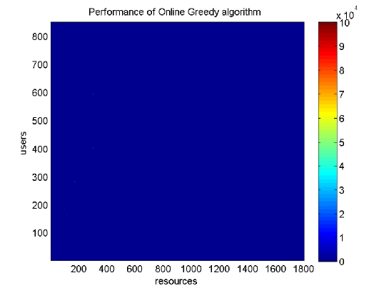
Figure 2: Cost vs Online Greedy

Figure 3: Cost vs Online Randomized

The weights of edges are initialized to zero. The availabilities of edges are initialized to the capacity of the producers connected. For greedy algorithm, the program chooses the available edge with the least cost. For the randomized algorithm, the program first sorts the available edges in increasing order. Then picks an edge suggested by the srand() and rand() function such that the cost of this edge is less than $\beta$ times the best available edge.

The weight of the edge returned - $weight(e)$, is increased by the value of demand and the availability $avail(e)$ is decreased by the same value. If there are any edge failures at the current demand the program generates a new internal demand and sets $avail(e)=weight(e)=0$ for the edge that failed. The program writes the total cost along with the $weight(e),\forall e\in E$ to the output file. STL map data-structures with double data-types are used for edge and node properties. STL 2-D vectors with double data-types are used for tracking the weights allocated on the edges for each consumer.

For finding the optimal offline solution in the case of edge failures additional constraints are added to LP at each instance of edge failure, such that the currently allocated weights are not disturbed. This is done for each of the edge failures with the demand of the consumers at each stage being equal to their sum of demands until the edge failed.

7.1 Analysis of Simulation Results

In Fig. 1 as the number of users increases with the same number of resources, the cost of the optimal offline also increases. The number of incoming edges to any producer increases as the consumers increase. This increases the competition for the resources available at the producers. The optimal offline algorithm has to select costlier edges due to limited availability of edges, as the number of demands increase and this increases the overall cost. This is inline with Fig 4 in [33] where it is referred to the latency (which is the overall time required to complete I/O requests).

Greedy algorithm Fig. 2 closely follows the optimal offline algorithm at each step of the input. greedy which produces output that has a cost comparable to the optimal solution and does not deviate much apart from the cases where higher demands arrive later as described in paragraph 2 in section 6.1.

Randomized algorithm does better than Greedy algorithm in cases where higher demands arrive later in the sequence. In this case, greedy algorithm fails badly as it does not have any cheaper edges left towards the end and has to select costlier edges for higher demands. However, Randomized algorithmFig. 3 does not cope well for graphs with higher number of nodes. Randomized algorithm pays the penalty of selecting a suboptimal edge to get an overall cost improvement; however due to large size of the demands it is not able to recover from this penalty and this causes a cascading effect. In Fig.3 the randomized online algorithm shows the highest standard deviation because of the random nature of the selections.

8 Conclusion

This paper concludes that it is possible to produce a competitive online algorithm for this problem using randomization. The competitiveness of this algorithm suffers for higher number of nodes and edges in the graph. This paper believes that it is possible to produce a competitive version of this algorithm by setting the suboptimal penalty to zero at the beginning of the algorithm and iteratively increasing it depending on the effect on the cost of the output.

9 Appendix

The results found this paper are based on the simulation experiments. It will be interesting to measure the performance of these online algorithms for real-world I/O demands. And, how it scales with the size of input.

Work on solving other versions of this problem where the distances $d_{ij}$s of edges may change over time is currently in progress.

10 Glossary

Definition 1

Dynamic graphs: Graphs that have a finite set of nodes and edges but where, the edges or nodes may become unavailable and available over time.

Definition 2

Derandomization: Process of removing randomness from an algorithm to make it more deterministic.

Definition 3

Assignment problem: Given a bipartite graph with tasks and resource on either side and a cost associated with allocating a task to a resource, the assignment problem is used to find the optimal allocation of the resources to the tasks (to minimize a Objective function)

Definition 4

Linear programming: A method used to solve large scale optimization problems with set constraints and objective function (minimize or maximize a quantity)

Definition 5

Combinatorial optimization: A certain class of optimization problems that involves minimization of a Objective function where there are multiple choices available at each step.

References

- [1] Kuhn HW, The Hungarian method for the assignment problem, Naval Research Logistics, Quarterly 2, 1955, 83–97.
- [2] Toroslu IH, ¨Uc¸ Oluk G, Incremental assignment problem, Information Sciences, 177, 6 (March 2007), 1523–1529.
- [3] B. Fuchs, W. Hochstattler, and W. Kern, Online matching on a line, Theoretical Computer Science 332 (1-3), 2005.
- [4] Adam Meyerson, Akash Nanavati, Laura Poplawski, Randomized online algorithms for minimum metric bipartite matching, Proceedings of the seventeenth annual ACM-SIAM symposium on Discrete algorithms, 954 - 959, 2006.
- [5] S. Khuller, S. Mitchell, and V. Vazirani, On-line algorithms for weighted bipartite matching and stable marriages, Theory of Computer Science 127(2), 1994.
- [6] Garg N, Kumar A, Better algorithms for minimizing average flow-time on related machines, Automata, Languages and Programming, Pt. 1, Lecture Notes in Computer Science, 4051, 181-190, 2006.
- [7] Ahuja RK, Orlin JB, Stein C, et al., Improved algorithms for bipartite network flow, SIAM Journal on Computing, 23, 5, 906-933, Oct 1994.
- [8] Goldberg AV, Plotkin SA, Shmoys DB, et al., Using interior-point methods for fast parallel algorithms for bipartite matching and related problems, SIAM Journal on Computing, 21, 1, 140-150, Feb 1992.
- [9] Correa JR, Wagner MR, LP-based online scheduling: From single to parallel machines, Integer programming and combinatorial optimization, proceedings, lecture notes in computer science, 3509, 196-209, 2005.
- [10] Amir Y, Awerbuch B, Barak A, Borgstrom RS, Keren A, An opportunity cost approach for job assignment in a scalable computing cluster, IEEE transactions on parallel and distributed systems 11, 7, 760-768, Jul 2000.
- [11] Spivey MZ, Powell WB, The dynamic assignment problem, Transportation Science 38, 4, November 2004, 399–419.
- [12] Monika R. Henzinger, Valerie King, Randomized fully dynamic graph algorithms with polylogarithmic time per operation, Journal of the ACM (JACM) archive, 46, 4, 502 - 516, July 1999.
- [13] David Alberts, Giuseppe Cattaneo, Giuseppe F. Italiano, An empirical study of dynamic graph algorithms, Journal of Experimental Algorithmics (JEA) archive, 2, article 5, 1997.
- [14] Aleksander Madry, Faster approximation schemes for fractional multicommodity flow problems via dynamic graph algorithms, Annual ACM Symposium on Theory of Computing archive, 2, Session 2A, 121-130, 2010.
- [15] Waldspurger CA, Hogg T, Huberman BA, et al., Spawn - A Distributed Computational Economy, IEEE Transactions on Software Engineering, 18 , no. 2, 103-117, Feb 1992 .
- [16] Baruah SK, Cohen NK, Plaxton CG, Varvel DA, Proportionate progress- A notion of fairness in resource allocation, Algorithmica, 15, 6, 600-625, Jun 1996 .
- [17] Azar Y, Broder AZ, Karlin AR, Upfal E, Balanced allocations, SIAM Journal of Computing, 29,1, 180-200, Sep 1999 .
- [18] S. Ben-David, A. Borodin, R. Karp, G. Tardos, A. Wigderson, On the Power of Randomization in On-line Algorithms, Algorithmica, vol. 11, no. 1, pp. 2-14, 1994.
- [19] Bar-Noy A, Bellare M, Halldorsson MM, Shachnai H, Tamir T, On chromatic sums and distributed resource allocation, Information and Computation 140, 2, 183-202, Feb 1 1998.
- [20] Kuchcinski K, Constraints-driven scheduling and resource assignment ACM transactions on design automation of electronic systems, 8, 3, 355-383, Jul 2003.
- [21] Aydin ME, Fogarty TC, A distributed evolutionary simulated annealing algorithm for combinatorial optimization problems Journal of Heuristics, 10, 3, 269-292, May 2004.
- [22] Buyya R, Yeo CS, Venugopal S, Broberg J, Brandic I, Cloud computing and emerging IT platforms: Vision, hype, and reality for delivering computing as the 5th utility, Future Generation Computer Systems-The International Journal of Grid Computing-Theory Methods And Applications, 25, 6, 599-616, Jun 2009.
- [23] Berman P, Charikar M, Karpinski M, On-line load balancing for related machines, Journal of Algorithms, 35, 1, 108-121, Apr 2000.
- [24] Phillips S, Westbrook J, On-line load balancing and network flow Algorithmica, 21, 3, 245-261, Jul 1998.
- [25] Tomislav Rudec, Alfonzo Baumgartner, Robert Manger, A fast implementation of the optimal off-line algorithm for solving the k-server problem, Math. Commun., 14, No. 1, pp. 119-134 (2009).
- [26] Irene Fink, Sven O. Krumke, Stephan Westphal, New lower bounds for online k-server routing problems, Information Processing Letters 109 (2009) 563–567.
- [27] Mark S. Manasse, Lyle A. McGeoch, Daniel D. Sleator, Competitive algorithms for server problems, Journal of Algorithms, 11 , Issue 2 (June 1990), 208 - 230.
- [28] Steven S. Seiden, A General Decomposition Theorem for the k-Server Problem, Information and Computation 174, 193–202 (2002).
- [29] Vincenzo Bonifaci, Leen Stougie, Online k-Server Routing Problems, Theory Comput Syst (2009) 45, 470–485.
- [30] Yair Bartal, Manor Mendel, Randomized k-server algorithms for growth-rate bounded graphs, Journal of Algorithms 55 (2005) 192–202.
- [31] Bar-Noy A, Freund A, Naor JS, On-line load balancing in a hierarchical server topology, SIAM Journal on Computing, 31, 2, 527-549, Oct 2001.
- [32] Dynamic Storage Provisioning, VMware, Nov 18, 2009.
- [33] Scalable Storage Performance, VMware, Jun 5, 2008.
- [34] lpsolve, Open source (Mixed-Integer) Linear Programming system, Multi-platform, pure ANSI C / POSIX source code, Lex / Yacc based parsing, Version 5.1.0.0 dated 1 May 2004, Michel Berkelaar, Kjell Eikland, Peter Notebaert, GNU LGPL (Lesser General Public Licence).