A Brief Introduction to Band Structure in Three Dimensions

Abstract

Without our ability to model and manipulate the band structure of semiconducting materials, the modern digital computer would be impractically large, hot, and expensive. In 8.06, we studied the effect of spatially periodic potentials on the spectrum of a charged particle in one dimension. We would like to understand how to extend these methods to model actual crystalline materials. Along the way, we will explore the construction of periodic potentials in three dimensions, and we use this framework to relate the single-particle Hamiltonian to the potential contribution from each atom. We then construct a crude model system analogous to the semiconductor silicon, and demonstrate the appearance of level splitting and band gaps as the strength of the potential is varied, in accordance with our intuition from the one-dimensional case. We discuss refinements of the model to include many-particle effects, and finally we show how a careful choice of the potential function leads to good agreement with the correct band diagram for silicon.

I Introduction

Many world-changing results from solid state physics, like the development of the silicon transistor, take advantage of the band structure of crystalline materials to give engineers detailed control over material behavior. Because crystals are ultimately many-particle systems with many degrees of freedom, the models that are used to describe these materials make a wide range of approximations in order to obtain mathematically and computationally tractable results about band structure. The most detailed models can predict not only the number and spacing of bands and the density of available states in the material, quantities useful for understanding the behavior of electrons near the Fermi surface at nonzero temperature, but also the effects of mechanical strain, defects, and impurities on the crystal’s electronic properties. Semiconductor engineers fit these models to empirical data to obtain very nuanced control over the behavior of devices.

In 8.06, we explored the behavior of single electrons in one-dimensional periodic potentials. This toy model allowed us to invoke several of the most important techniques for learning about band structure, including the nearly-free electron model, which explained how tiny interactions between otherwise free valence electrons can open up band gaps, and the tight-binding model, which showed that even closely-held core electrons undergo level splitting to form narrow bands.

In this work, we will show how these techniques generalize from one dimension to three dimensions, demonstrating the appearance of level splitting and band gaps as a periodic potential is gradually “switched on”. We will also show how an approximation to the correct band structure of the semiconductor silicon can be obtained within this model by adjusting the potential function.

In order to apply the nearly-free electron model, we will need a mathematical framework for the three-dimensional lattice. We can then take a periodic potential on this lattice over to the Fourier domain, recovering the reciprocal lattice. This will tell us how the Brillouin zone generalizes to three dimensions. After reviewing Bloch’s theorem, we will put all of these pieces together to find and solve the Hamiltonian for a particle moving in a three-dimensional periodic potential, and consider briefly how this approach can be extended to the many-particle case.

II Lattice Formalism

II.1 Bravais Lattice

Consider the potential energy of an electron located at a point $\vec{x}$ within an infinite grid of positively-charged ions, all carrying the same charge. We can write this as

$$V(\vec{x})=\sum_{i}U(\vec{x}-\vec{x}_{i})$$ (1)

where $x_{i}$ is the position of the $i^{\mathrm{th}}$ atom, and $U(\vec{x})$ is the potential due to a single ion at the origin. In one dimension, we write the positions of the atoms as

$$\vec{x}_{n}=na\hat{x}=n\vec{a}_{1}$$ (2)

for integer $n$, where $a$ is the lattice spacing, and we have defined $\vec{a}_{1}\equiv a\hat{x}$. The region of 1-D space bounded by $(0,a)$ is a unit cell.

Notice that there is no particular reason to require that $U(\vec{x})$ be the potential due to a single ion. One could construct a 1-D crystal where small, identical clusters of atoms form a repeating pattern with period $a$, with each cluster containing several atoms spaced by less than $a$.

In three dimensions, the situation is more interesting, since we have some freedom to define the directions along which the crystal is periodic (they don’t necessarily have to be perpendicular). Even for oblique directions of periodicity, we can write

$$\vec{x}_{n,m,\ell}=n\vec{a}_{1}+m\vec{a}_{2}+\ell\vec{a}_{3}$$ (3)

to give the positions of a regular grid of points. Families of points describable in these terms are called Bravais lattices. Common Bravais lattices include the cubic lattice system (simple, body-centered, and face-centered) and the hexagonal lattice. The cubic lattice system is shown in Figure 1(a), (b), and (c), with circles indicating the locations of atoms in the simple, body-, and face-centered cubic configurations, respectively. You should take a moment to convince yourself that shifting the origin by one step along any of the indicated directions of periodicity $\vec{a}_{1,2,3}$ leaves the lattice unchanged.

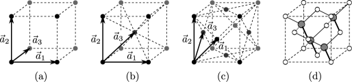
Figure 1: Cubic Bravais lattice system: (a) simple cubic, (b) body-centered cubic, (c) face-centered cubic. The vectors $\vec{a}_{1,2,3}$ represent directions of periodicity. The unit cells contain 1, 2, and 4 points, respectively. (d) Diamond cubic variation, with additional atoms highlighted. The lines illustrate the tetrahedral symmetry about each atom. Atoms in (d) connected by a thick line are associated with the same lattice point.

As in the 1-D case, it should be stressed that the potential $U(\vec{x})$ can describe a cluster containing more than one ion. For instance, diamond, silicon, germanium, and the allotrope $\alpha$-tin adopt a crystal structure that positions two atoms at each point of a face-centered cubic (FCC) lattice. This structure, known as “diamond cubic”, is shown in Figure 1(d).

II.2 Bloch’s Theorem

If a Hamiltonian commutes with a set of unitary, mutually commuting translation operators $\hat{T}_{\vec{a}}$, then the eigenstates of $\mathcal{H}$ can be chosen to be (simultaneously) eigenstates of all the $\hat{T}_{\vec{a}}$. This follows because hermitian and unitary operators are normal operators, and a set of normal operators commutes if and only if it is simultaneously diagonalizable (an extention of our 8.05 result for commuting hermitian operators). Now any two translation operators of the form $\hat{T}_{\vec{a}}=\exp(-i\hat{\vec{p}}\cdot\vec{a}/\hbar)$ commute, since the individual components of $\hat{\vec{p}}$ commute. Furthermore, since the translation operators are unitary, their eigenvalues have unit magnitude.

Suppose that $\mathcal{H}$ can be written as the sum of a kinetic term $\hat{\vec{p}}\,^{2}/2m$ and a potential term which satisfies $V(\vec{x})=V(\vec{x}+\vec{a})$ for some set of $\vec{a}$. Then $[\mathcal{H},\hat{T}_{\vec{a}}]=0$, and we can find an eigenbasis for $\mathcal{H}$ which satisfies

$$\hat{T}_{\vec{a}}|\psi\rangle=e^{i\theta_{\vec{a}}}|\psi\rangle$$ (4)

for $\vec{a}$ in our set.

We know that composing two translation operators $\hat{T}_{\vec{a}}$ and $\hat{T}_{\vec{b}}$ gives $\hat{T}_{\vec{a}+\vec{b}}$. To maintain consistency with (4), $\theta_{\vec{a}}$ must be linear in $\vec{a}$. We will take

$$\theta_{\vec{a}}\equiv-\kappa\cdot\vec{a}$$ (5)

This gives

$$\langle\vec{x}|\hat{T}_{\vec{a}}|\psi\rangle =e^{-i\kappa\cdot\vec{a}}\langle\vec{x}|\psi\rangle$$

$$\psi(\vec{x}-\vec{a}) =e^{-i\kappa\cdot\vec{a}}\psi(\vec{x})$$

So we see that the eigenstates of $\mathcal{H}$ can be written in the spatial basis as

$$\psi(\vec{x})=e^{i\vec{\kappa}\cdot\vec{x}}u(\vec{x})$$ (6)

where $u(\vec{x})=u(\vec{x}+\vec{a})$ for all $\vec{a}$ in our set.

II.3 Reciprocal Lattice

When we apply Bloch’s theorem to the potential (1), we find that the wavefunction can be written in terms of a function $u(\vec{x})$ which has the same periodicity as the lattice:

$$u(\vec{x})=u(\vec{x}+n\vec{a}_{1}+m\vec{a}_{2}+\ell\vec{a}_{3})\;\forall\;n,m,\ell\in\mathbb{Z}$$ (7)

It is productive to ask whether the Fourier transform of such a function (that is, its representation in the momentum basis) has any helpful properties. Starting with

$$u(\vec{x})=u(\vec{x}+\vec{a})$$

for some $\vec{a}$, and writing each side in terms of the inverse transform of $\widetilde{u}(\vec{k})$, we find

$$\int d^{3}\vec{k}e^{i\vec{k}\cdot\vec{x}}\widetilde{u}(\vec{k})=\int d^{3}\vec{k}e^{i\vec{k}\cdot\vec{x}}e^{i\vec{a}\cdot\vec{k}}\widetilde{u}(\vec{k})$$

Collecting terms and taking the inverse transform gives

$$0=(1-e^{i\vec{a}\cdot\vec{k}})\widetilde{u}(\vec{k})$$

from which it follows that

$$\forall\vec{k},\text{ either }\vec{a}\cdot\vec{k}=2\pi N\text{ for some $N\in\mathbb{Z}$, or }\widetilde{u}(\vec{k})=0.$$

This result shows that if a function is periodic in $\vec{a}$, then its transform must be zero everywhere except where $\vec{a}\cdot\vec{k}$ is a multiple of $2\pi$. This can be summarized by saying that periodic functions have discrete transforms.

In three dimensions, we have three linearly independent directions of periodicity, and hence three discreteness constraints on the $\vec{k}$ where $\widetilde{u}(\vec{k})$ is allowed to be nonzero. Writing $\vec{a}\cdot\vec{k}$ as $a^{\mathsf{T}}\vec{k}$, we can combine the three constraints into one matrix expression:

$$\left[\begin{matrix}a_{1}^{\mathsf{T}}\\ a_{2}^{\mathsf{T}}\\ a_{3}^{\mathsf{T}}\end{matrix}\right]\vec{k} =2\pi\left[\begin{matrix}N\\ M\\ L\end{matrix}\right]$$

$$\rightarrow\vec{k} =2\pi\left[\begin{matrix}a_{1}^{\mathsf{T}}\\ a_{2}^{\mathsf{T}}\\ a_{3}^{\mathsf{T}}\end{matrix}\right]^{-1}\left[\begin{matrix}N\\ M\\ L\end{matrix}\right]$$

If we define $\vec{g}_{1,2,3}$ to be $2\pi$ times the three columns of the inverse matrix, then we have an expression for a new Bravais lattice:

$$\vec{k}=N\vec{g}_{1}+M\vec{g}_{2}+L\vec{g}_{3}$$ (8)

Each $\vec{k}$ vector allowed by this lattice corresponds to a complex exponential $e^{i\vec{k}\cdot\vec{x}}$ in real space which is periodic in $\vec{a}_{1,2,3}$. This structure is called the reciprocal (or dual) lattice, and the space it occupies has many names: it is alternatively called reciprocal space, dual space, $\vec{k}$-space, transform space, or (loosely) momentum space. From now on, we will refer to the original Bravais lattice as the real space lattice. Curiously, if the real space lattice is face-centered cubic, the reciprocal lattice turns out to be body-centered cubic, and vice versa.

The preceding argument established that the Fourier transform of a periodic function is nonzero only on the reciprocal lattice. If we write the potential (1) as a convolution product,

$$V(\vec{x})=U(\vec{x})*\sum_{n,m,\ell}\delta(\vec{x}-n\vec{a}_{1}-m\vec{a}_{2}-\ell\vec{a}_{3})$$

we can take the Fourier transform of the two factors separately to obtain

$$\widetilde{V}(\vec{k})=\widetilde{U}(\vec{k})\sum_{n,m,\ell}e^{-i\vec{k}\cdot(n\vec{a}_{1}+m\vec{a}_{2}+\ell\vec{a}_{3})}$$

When we carry out the summation, we get a new sum over the reciprocal lattice, which we can again write in matrix form:

$$(2\pi)^{3}\!\!\!\sum_{N,M,L}\!\! \delta(\vec{k}\cdot\vec{a}_{1}\!-\!2\pi N)\delta(\vec{k}\cdot\vec{a}_{2}\!-\!2\pi M)\delta(\vec{k}\cdot\vec{a}_{3}\!-\!2\pi L)$$

$$=(2\pi)^{3}\sum_{N,M,L}\delta\left(\left[\begin{matrix}a_{1}^{\mathsf{T}}\\ a_{2}^{\mathsf{T}}\\ a_{3}^{\mathsf{T}}\end{matrix}\right]\vec{k}-2\pi\left[\begin{matrix}N\\ M\\ L\end{matrix}\right]\right)$$

Finally, we can show by $u$-substitution that this is just

$$\frac{(2\pi)^{3}}{\mathrm{det}\left|a_{1}a_{2}a_{3}\right|}\sum_{G}\delta(\vec{k}-\vec{G})$$

where $\sum_{G}$ is over the reciprocal lattice. So

$$\widetilde{V}(\vec{k}) =\widetilde{U}(\vec{k})\frac{(2\pi)^{3}}{\mathrm{det}\left|a_{1}a_{2}a_{3}\right|}\sum_{G}\delta(\vec{k}-\vec{G})$$

$$=\frac{(2\pi)^{3}}{\Omega}\sum_{G}U_{G}\,\delta(\vec{k}-\vec{G})$$ (9)

where we have defined $U_{G}\equiv\widetilde{U}(\vec{G})$ and $\Omega\equiv\mathrm{det}\left|a_{1}a_{2}a_{3}\right|$.

II.4 First Brillioun Zone

Our study of Bloch’s theorem led us to wavefunctions of the form $\psi(\vec{x})=e^{i\vec{\kappa}\cdot\vec{x}}u(\vec{x})$, with $u(\vec{x})$ periodic in real space. But we just observed that every $e^{i\vec{G}\cdot\vec{x}}$ with $\vec{G}$ on the reciprocal lattice is periodic in real space. Thus if we write $\psi^{\prime}(\vec{x})=e^{i(\vec{\kappa}-\vec{G})\cdot\vec{x}}(e^{i\vec{G}\cdot\vec{x}}u(\vec{x}))=e^{i\vec{\kappa}^{\prime}\cdot\vec{x}}u^{\prime}(\vec{x})$, we obtain an equally valid expression for the exact same wavefunction. In this sense, $\vec{\kappa}$ is not really a free parameter of the system, but can be restricted without loss of generality to lie in a small region of the reciprocal space. Conventionally, we choose this region to contain all vectors $\vec{\kappa}$ which are closer to $\vec{G}=0$ than to any other reciprocal lattice point. If we start with a $\vec{\kappa}$ closer to some other reciprocal lattice point $\vec{G}\neq 0$, we can subtract $\vec{G}$ from it to get an equivalent point closest to $0$. The region of space closer to $0$ than to any other reciprocal lattice point is called the first Brillouin zone. In one dimension it was given by the interval $(-\frac{\pi}{a},\frac{\pi}{a})$, since the boundaries between regions in one dimension are simply points. In three dimensions, these boundaries are planes, and the first Brillouin zone has a rather beautiful shape formed by the intersections of boundary planes. The first Brillouin zone for an FCC real space lattice is shown in Figure 2. This polyhedron bounds the region of reciprocal space where we will focus our attention.

The job of a band structure diagram is to summarize all the interesting things going on in $\vec{k}$-space. Since it is difficult to capture all the features of a volume on a flat piece of paper, these diagrams typically take a little tour around the first Brillouin zone, following a (somewhat) standardized trajectory. You will notice that a number of particularly symmetric points in the figure have been named with capital Roman and Greek letters. These letters will appear along the horizontal axis of band structure diagrams, and it is understood that motion along the horizontal axis corresponds to progress along a trajectory between these points of symmetry in $\vec{k}$-space. For instance, the segment of the graph labeled $\Gamma$–$X$ corresponds to the straight line in $\vec{k}$-space from $\vec{k}=0$ to $\vec{k}=(2\pi/a)\hat{x}$.

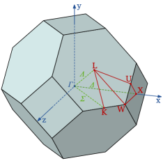
Figure 2: First Brillouin zone for a face-centered cubic real space lattice. Represents the volume in $\vec{k}$-space closer to $\vec{0}$ than to any other reciprocal lattice vector, and includes all the Bloch wave vectors $\vec{\kappa}$ necessary to describe the band structure of the crystal.

III Nearly-Free Electron Model

We would like to write down and solve the Hamiltonian for a single particle moving in a periodic potential. While it is not true in general that the dynamics of a many-electron system can be described in terms of one set of single-particle states, single-particle wavefunctions are nevertheless a useful tool for approximating the correct many-particle system.

Working in the plane wave basis, we will find an expression for the matrix elements of the Bloch Hamiltonian in terms of the Fourier transform of the potential. We neglect electron-electron interactions. Later on, we will show how to interpret this approximation as an application of the variational principle.

III.1 Basis

Our orthogonal basis and normalization convention are

$$\langle\vec{x}|\vec{x}^{\prime}\rangle =\delta(\vec{x}-\vec{x}^{\prime})$$

$$|\vec{k}\rangle =\int d^{3}\vec{x}e^{i\vec{k}\cdot\vec{x}}|\vec{x}\rangle$$ (10)

$$\langle\vec{k}|\vec{k}^{\prime}\rangle =\int d^{3}\vec{x}\int d^{3}\vec{x}^{\prime}\langle\vec{x}|e^{-i\vec{k}\cdot\vec{x}}e^{i\vec{k}^{\prime}\cdot\vec{x}^{\prime}}|\vec{x}^{\prime}\rangle$$

$$=(2\pi)^{3}\delta(\vec{k}-\vec{k}^{\prime})$$ (11)

III.2 Hamiltonian

We begin with the Hamiltonian for a particle in an arbitrary potential.

$$\mathcal{H}=\frac{\hat{\vec{p}}\,^{2}}{2m}+V(\hat{\vec{x}})$$ (12)

Using the fact that $\left[\mathcal{H},\hat{T}_{\vec{a}}\right]=0$ for any translation $\vec{a}$ in the real space lattice and applying Bloch’s theorem, we can write the eigenstates $|\psi\rangle$ as

$$|\psi\rangle=e^{i\vec{\kappa}\cdot\hat{\vec{x}}}|u_{\vec{\kappa}}\rangle$$ (13)

where $u_{\vec{\kappa}}(\vec{x})$ has the same periodicity as the real space lattice, and the Schrödinger equation is written as

$$\mathcal{H}_{\mathrm{eff}}|u_{\vec{\kappa}}\rangle =E|u_{\vec{\kappa}}\rangle$$ (14)

$$\mathcal{H}_{\mathrm{eff}} =\frac{1}{2m}(\hat{\vec{p}}+\hbar\vec{\kappa})^{2}+V(\hat{\vec{x}})$$ (15)

Using the plane wave basis for $|u_{\vec{\kappa}}\rangle$, we find matrix elements

$$\langle\vec{k}|\mathcal{H}_{\mathrm{eff}}|\vec{k}^{\prime}\rangle=\frac{\hbar^{2}}{2m}(\vec{k}+\vec{\kappa})^{2}\langle\vec{k}|\vec{k}^{\prime}\rangle+\langle\vec{k}|V(\hat{\vec{x}})|\vec{k}^{\prime}\rangle$$ (16)

We can write $V(\hat{\vec{x}})$ in terms of $\widetilde{V}(\vec{x})$ with the help of (9):

$$V(\hat{\vec{x}}) =\frac{1}{(2\pi)^{3}}\int d^{3}\vec{k}V(\vec{k})e^{i\vec{k}\cdot\hat{\vec{x}}}$$

$$=\frac{1}{\Omega}\sum_{G}U_{G}\int d^{3}\vec{k}\delta(\vec{k}-\vec{G})e^{i\vec{k}\cdot\hat{\vec{x}}}$$

Using the sifting property of the delta function,

$$V(\hat{\vec{x}})=\frac{1}{\Omega}\sum_{G}U_{G}e^{i\vec{G}\cdot\hat{\vec{x}}}$$

We can now find matrix elements for our potential using the definition of $|\vec{k}\rangle$:

$$\langle\vec{k}|V(\hat{\vec{x}})|\vec{k}^{\prime}\rangle =\frac{1}{\Omega}\sum_{G}U_{G}\!\!\int\!d^{3}\vec{x}\!\int d^{3}\vec{x}^{\prime}\langle\vec{x}|e^{-i\vec{k}\cdot\vec{x}}e^{i\vec{G}\cdot\hat{\vec{x}}}e^{i\vec{k}^{\prime}\cdot\vec{x}^{\prime}}|\vec{x}^{\prime}\rangle$$

$$=\frac{1}{\Omega}\sum_{G}U_{G}\!\!\int\!d^{3}\vec{x}e^{i\vec{x}\cdot(\vec{G}-\vec{k}+k^{\prime})}$$

Taking the integral, we have

$$\langle\vec{k}|V(\hat{\vec{x}})|\vec{k}^{\prime}\rangle=\frac{1}{\Omega}(2\pi)^{3}\sum_{G}U_{G}\delta(\vec{G}-\vec{k}+k^{\prime})$$ (17)

Computations in a continuous basis like $|\vec{k}\rangle$ are problematic because they are difficult to approximate numerically. We would much rather work in a vector space with a discrete basis, so that our linear operators become ordinary matrices. Fortunately, the structure of (17) permits us to divide the continuous basis into a set of discrete subspaces, with the assurance that there will be no coupling between subspaces. In matrix terminology, our Hamiltonian is block diagonal. Using this fact, we can easily restrict the action of the Hamiltonian to a given subspace and solve numerically.

From (17), we can see that the Hamiltonian (15) couples states $|\vec{k}\rangle$ and $|\vec{k}^{\prime}\rangle$ if they differ by a reciprocal lattice vector. Otherwise, the off-diagonal matrix elements vanish. Thus, to every $\vec{k}$ in the first Brillouin zone there corresponds a family of states $|\vec{k}+\vec{G}\rangle$ which are (potentially) coupled by the potential. Without losing any physics, we can restrict the Hamiltonian to act in one of these discrete orthonormal subspaces by constructing (and normalizing) matrix elements

$$\frac{\langle\vec{k}+\vec{G}|V(\hat{\vec{x}})|\vec{k}+\vec{G}^{\prime}\rangle}{\sqrt{\langle\vec{k}+\vec{G}^{\prime}|\vec{k}+\vec{G}^{\prime}\rangle\langle\vec{k}+\vec{G}|\vec{k}+\vec{G}\rangle}} =\frac{\frac{1}{\Omega}(2\pi)^{3}U_{G-G^{\prime}}\delta(0)}{\sqrt{(2\pi)^{3}\delta(0)(2\pi)^{3}\delta(0)}}$$

$$=\frac{1}{\Omega}U_{G-G^{\prime}}$$ (18)

We can build one of these matrices for each $\vec{k}$ we are interested in, add $\hbar^{2}(\vec{k}+\vec{G})^{2}/2m$ to the diagonal, and we will have the full Hamiltonian for the corresponding subspace.

Now that we have matrix elements, why don’t we apply perturbation theory? If the potential is small compared to $\hbar^{2}(\vec{k}+\vec{\kappa})^{2}/2m$, we can view it as a perturbation on the Hamiltonian for a free particle. In order to obtain corrections to the free particle energies and wavefunctions, we must first look for the “good” states, that is, the basis in which the perturbation is diagonal within every degenerate subspace of the unperturbed Hamiltonian. We know that the degenerate subspaces of the unperturbed (free) Hamiltonian correspond to spheres of constant $|\vec{k}|$ in momentum space. The question is whether the matrix element of $V(\hat{\vec{x}})$ between two states on the same sphere is nonzero. Since a sphere has chords of every length in $(0,2r]$, we can see by (18) that any vector $\vec{G}$ in the reciprocal lattice which is short enough to fit inside the sphere (that is, with $0<|\vec{G}|\leq 2|\vec{k}|$) couples together degenerate states. Certain special potentials, for instance those which are periodic in $x$ but constant in $y$ and $z$, permit us to choose a sine and cosine basis that diagonalizes $V(\hat{\vec{x}})$. For more general potentials, finding a good basis is bothersome. At this point, the easiest thing to do is to throw the problem at a computer. We have to make a few more decisions – most importantly, what our potential function $U(\vec{x})$ is, and how many states $|\vec{k}+\vec{G}\rangle$ to include in the truncated (finite) matrix form of $\mathcal{H}_{\text{eff}}$ – but given these, finding the single-particle energies and wavefunctions is a simple matter of computing each matrix element numerically using (18), and then invoking a subroutine to find the eigenvalues and eigenvectors of this matrix. Fast and accurate subroutines to perform this function are present in every standard linear algebra system. In the popular LAPACK library (Linear Algebra PACKage), for instance, there is a subroutine called zheevd that does what we want. To generate a band structure diagram, we will need to compute and plot these eigenvalues for each $\vec{k}$ we encounter on our tour of the first Brillouin zone.

IV Model System

Using the framework we have developed, we can now choose a particular system and plot some band diagrams to verify our work and improve our intuition into the phenomenology of band structure.

IV.1 Potential

As it turns out, a great deal of research Chelikowsky and Cohen (1976); Kresse and Furthmüller (1996); Tafipolsky and Schmid (2006); Bachelet et al. (1982); Pickett (1989) has gone into the choice of the potential function, since much of the actual many-particle physics can be incorporated by a suitable choice of $U(\vec{x})$. For instance, once we obtain wavefunctions for a crystal filled with non-interacting electrons, we can calculate the effect of e^-–e^- repulsion (classical) and correlation (the quantum “exchange force”). Treating these as an adjustment to the potential, the system can re-solved to obtain a set of wavefunctions that are sensitive to many-particle effects. These can in turn be used to make a better estimate of repulsion and correlation effects. The iterations stop when the wavefunction-dependent potential and the potential-dependent wavefunctions are mutually consistent. This is the Hartree-Fock method. The approximation here lies in the assumption that the many-particle ground state can be written as an antisymmetrized product of single-particle wavefunctions. In general, it is a linear combination of many such products. This makes Hartree-Fock a variational technique, since we are effectively minimizing the energy of a trial multi-particle wavefunction. The minimization is over all possible sets of single-particle states. Since the expectation value of the Hamiltonian on any state is an upper bound on the ground state, the Hartree-Fock method gives an upper bound on the energy of the crystal system.

For simplicity, we will use a Coulomb potential of the form

$$U(\vec{x})=-\frac{Z_{\text{eff}}q^{2}}{|\vec{r}|}$$ (19)

Since our goal is to model the diamond-cubic silicon crystal, we will have to add another Coulombic potential at an offset to represent the two-ions-per-lattice-site structure. Even this gross simplification (we haven’t considered e^-–e^- interactions, spin, etc.) is sufficient to capture some of the flavor of the correct band diagram. In any event, we’ll need the Fourier transform of this potential, so we’d better go ahead and compute it.

As it turns out, the Fourier integral for the function $-Z_{\text{eff}}q^{2}/r$ doesn’t converge. The transform of the related “Yukawa” potential $-Z_{\text{eff}}q^{2}e^{-mr}/r$ is

$$\widetilde{U}(\vec{k})=-Z_{\text{eff}}q^{2}\frac{4\pi}{k^{2}+m^{2}}$$ (20)

In the limit as $m\rightarrow 0$, we recover the transform of the Coulomb potential everywhere except at $\vec{k}=0$.

$$\widetilde{U}(\vec{k})=-Z_{\text{eff}}q^{2}\frac{4\pi}{k^{2}}$$ (21)

Since $U_{0}$ only appears on the diagonal of the Hamiltonian, ignoring the divergence at $\vec{k}=0$ corresponds to neglecting a constant energy shift.

IV.2 Results

Computed band structure diagrams for the diamond cubic crystal (Coulombic potential) are presented in Figure 3 for four different values of $Z_{\text{eff}}$. The labels along the horizontal axis correspond to $\vec{k}$-space points in the first Brillouin zone (Figure 2). Note especially that

• For a free electron, we expect $E=p^{2}/2m\propto k^{2}$. In fact, when $Z_{\text{eff}}=0$, we find parabolic dispersion around the point $\vec{k}=\Gamma=0$.

• Along the path $L$–$\Gamma$, we recover much the same “folded parabola” structure we saw in one dimension, with branches of the band diagram reflecting off the wall of the Brillouin zone (in this case, at $L$).

• For small $Z_{\text{eff}}$, the effects of the perturbation should be most visible near crossings and degenerate branches of the band diagram, where level repulsion is strongest. This effect is observed as expected. Note that even though the Coulomb potential gives nonzero Fourier components for every nonzero $\vec{k}$, not all degeneracies are broken. Part of the reason is due to zeros imposed by the two-atom-per-FCC-site diamond cubic structure.

• For a tightly bound electron (high $Z_{\text{eff}}$), we expect to find more or less isolated bands corresponding to the orbitals of isolated atoms. Since band spreading corresponds to tunneling in the tight binding picture, these bands describe localized states.

In Figure 4, we show how this simple model can incorporate the more complicated situation of many-particle interactions in an ad-hoc way. By selecting a few matrix elements essentially by hand, a very close correspondence can be obtained with results from more advanced literature Chelikowsky and Cohen (1976). In the literature, these matrix elements would be calculated, if not from first principles, then from fitting with experimental data such as x-ray reflectivity curves.

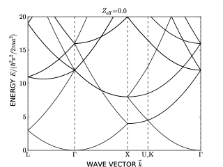
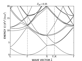
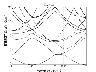
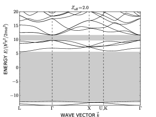
Figure 3: Level splitting and band gap formation in a diamond cubic crystal as the strength of the Coulombic potential is varied upwards from zero. From top left to bottom right, $Z_{\text{eff}}=0,0.25,0.5,2.0$. Energy gaps are shown in gray. Letters along the horizontal axis represent points in the first Brillouin zone (Figure 2).

$n^{2}$	$\hat{V}_{k,k+G}$
0	-9.50
12	-2.42
32	-0.80
44	-0.82
64	-0.88
76	-0.00

(a) Selected matrix elements $\hat{V}_{k,k+G}$ for a non-Coulombic potential, where $|G|=n\pi/a$. Units are electron volts. Remaining matrix elements are unchanged.

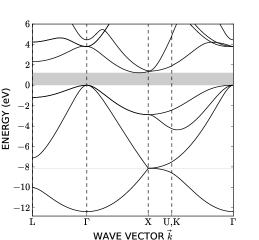
(a) Computed diamond cubic crystal band structure using the non-Coulombic potential described in 1(a).

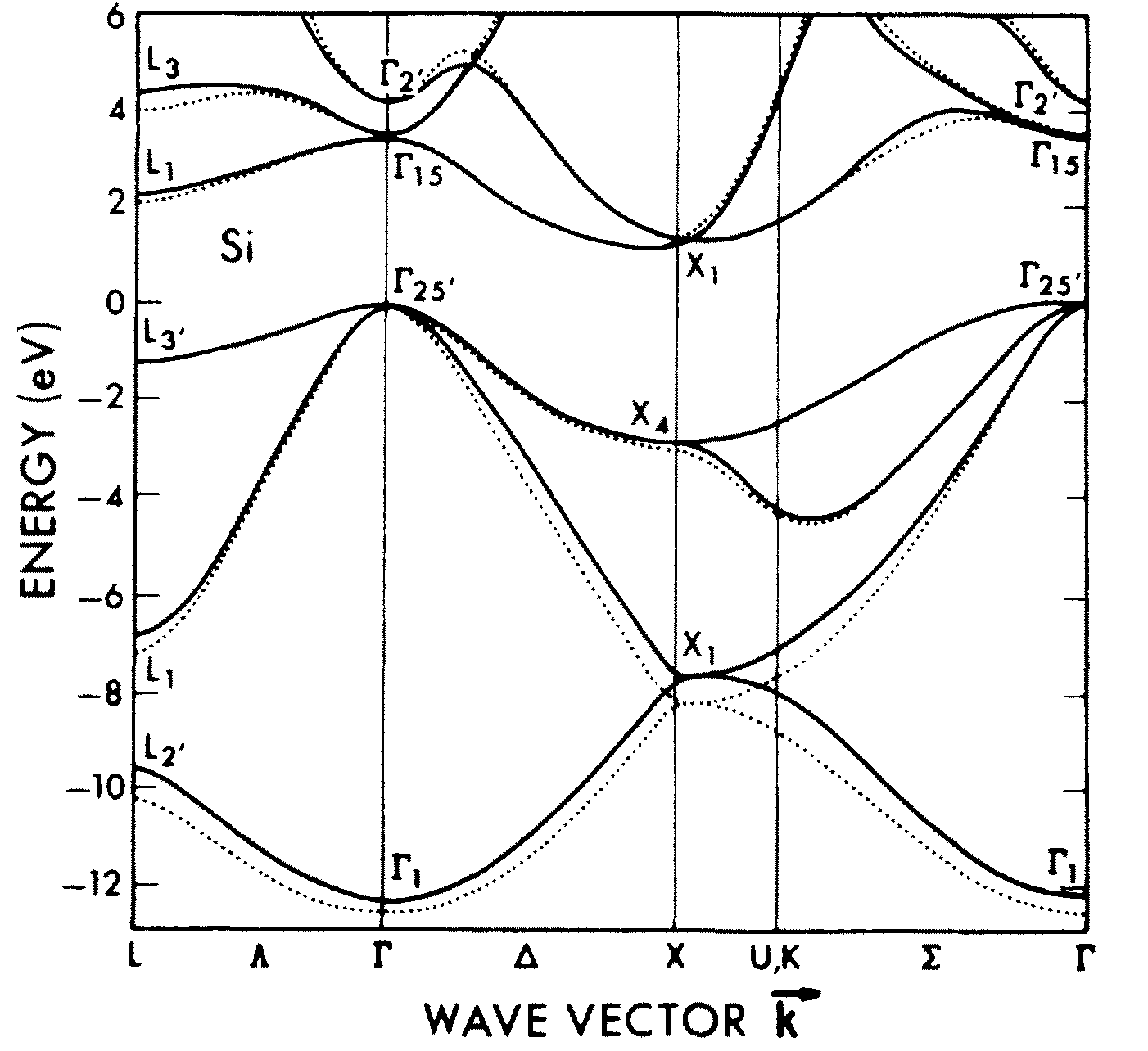
(b) Band structure for Si. Solid and dashed lines correspond to different techniques for incorporating e^-–e^- interations. Reproduced with permission from Chelikowsky and Cohen (1976). Copyright 1976 by The American Physical Society.

Figure 4: By modifying the potential, good agreement can be obtained with the band structure for Si shown in Figure 1 of Chelikowsky and Cohen (1976).

V Discussion

As we have seen, it is possible to get a lot of mileage out of the single-particle system. By adopting more sophisticated approaches to the potential due to e^-–e^- interactions, Chelikowsky and Cohen (1976) and many others have obtained models for band structure in real semiconductors with good accuracy and substantial predictive power. The single-particle framework we have developed is simplistic insofar as it ignores the effects of spin-orbit coupling, electron correlation, strains, electric and magnetic fields, impurities, and finite-temperature effects. It is nonetheless powerful enough to make contact with the more advanced literature when supplied with an ad-hoc choice of potential, and it remains beautiful in its simplicity.

Acknowledgements

The author is grateful to Nan Gu for conversations on finding matrix elements in the plane wave basis, and to Yan Zhu and Francesco D’Eramo for review and advice.

References

- Chelikowsky and Cohen (1976) J. R. Chelikowsky and M. L. Cohen, Phys. Rev. B 14, 556 (1976).
- Kresse and Furthmüller (1996) G. Kresse and J. Furthmüller, Phys. Rev. B 54, 11169 (1996).
- Tafipolsky and Schmid (2006) M. Tafipolsky and R. Schmid, The Journal of Chemical Physics 124, 174102 (pages 9) (2006).
- Bachelet et al. (1982) G. B. Bachelet, D. R. Hamann, and M. Schlüter, Phys. Rev. B 26, 4199 (1982).
- Pickett (1989) W. E. Pickett, Computer Physics reports 9, 115 (1989), ISSN 0167-7977.
- Cohen and Chelikowsky (1989) M. Cohen and J. Chelikowsky, Electronic structure and optical properties of semiconductors, Springer series in solid-state sciences (Springer-Verlag, 1989), ISBN 9780387188188.
- Blöchl (1994) P. E. Blöchl, Phys. Rev. B 50, 17953 (1994).
- Briggs et al. (1996) E. L. Briggs, D. J. Sullivan, and J. Bernholc, Phys. Rev. B 54, 14362 (1996).
- Ashcroft and Mermin (1976) N. W. Ashcroft and D. N. Mermin, Solid State Physics (Thomson Learning, Toronto, 1976), 1st ed., ISBN 0030839939.
- Kittel (2005) C. Kittel, Introduction to Solid State Physics (Wiley, New York, 2005), 8th ed., ISBN 0471111813.
- Hellmann (1935) H. Hellmann, The Journal of Chemical Physics 3, 61 (1935).
- Luttinger and Kohn (1955) J. M. Luttinger and W. Kohn, Phys. Rev. 97, 869 (1955).
- Hoddeson et al. (1992) L. Hoddeson, E. Braun, J. Teichmann, and S. Weart, Out of the crystal maze : chapters from the history of solid-state physics (Oxford University Press, New York , Oxford, 1992).
- Yu and Cardona (2005) P. Y. Yu and M. Cardona, Fundamentals of Semiconductors - Physics and Materials Properties (Springer, 2005), 3rd ed.
- Chelikowsky and Cohen (1974) J. R. Chelikowsky and M. L. Cohen, Phys. Rev. B 10, 5095 (1974).