Comparing the Topological and Electrical Structure of the North American Electric Power Infrastructure

Abstract

The topological (graph) structure of complex networks often provides valuable information about the performance and vulnerability of the network. However, there are multiple ways to represent a given network as a graph. Electric power transmission and distribution networks have a topological structure that is straightforward to represent and analyze as a graph. However, simple graph models neglect the comprehensive connections between components that result from Ohm’s and Kirchhoff’s laws. This paper describes the structure of the three North American electric power interconnections, from the perspective of both topological and electrical connectivity. We compare the simple topology of these networks with that of random Erdos:1959 , preferential-attachment Barabasi:1999 and small-world Watts:1998 networks of equivalent sizes and find that power grids differ substantially from these abstract models in degree distribution, clustering, diameter and assortativity, and thus conclude that these topological forms may be misleading as models of power systems. To study the electrical connectivity of power systems, we propose a new method for representing electrical structure using electrical distances rather than geographic connections. Comparisons of these two representations of the North American power networks reveal notable differences between the electrical and topological structure of electric power networks.

I Introduction

Recent research in complex networks Boccaletti:2006 has elucidated strong links between network structure and performance. Scale-free networks, which are characterized by strongly heterogeneous (power-law) node connectivity (degree), are uniquely robust to random failures but vulnerable to directed attacks Barabasi:1999 ; Albert:2000 . Graphs with exponential degree distributions, such as the random graph Erdos:1959 and small-world networks Watts:1998 are more equally vulnerable to random failures and directed attacks. Scale-free networks also tend to lose synchronization when attacked at hub nodes Wang:2002 , which is not the case for random graphs. And, for controllable networks, scale-free networks can be synchronized by controlling a small number of highly connected nodes Li:2004 , or even a single node Chen:2007 . On the other hand, ref. Atay:2006 shows that many classes of networks fail to synchronize, arguing that degree distribution alone is not sufficient to characterize the performance of a network. References Wu:1995 ; Wu:2005 describe how network structure influences consensus (a form of synchronization), and how different ways of representing a system a graph may affect the conclusions that one draws about performance. Others De-Lellis:2008 ; De-Lellis:2010a show that it is possible to maintain synchronization in evolving network topologies.

Given that network structure can dramatically influence performance, and given the size, complexity and importance of electric power systems, it is not surprising that power grids are the subject of substantial study from a complex networks perspective Dorfler:2010 . The fact that data from many countries show a power-law in power system blackout sizes Dobson:2007 , leads naturally to the conjecture that this might result from complexity in network structure. Watts and Strogatz Watts:1998 measure characteristic path length and clustering in power grids, and find similarities to the small-world network model. A number of studies measure the degree distribution of various power grids with some reporting exponential Amaral:2000 ; Albert:2004 ; Crucitti:2004 and others reporting power-law/scale-free degree distributions Barabasi:1999 ; Chassin:2005 . That studies of different power grids in different countries or regions yield different topological structures is not necessarily surprising. More surprising is that different analyses of identical grids (the transmission system in the Western U.S.) have yielded different structural results Albert:2004 ; Chassin:2005 . In particular, this discrepancy stems from the model used in Chassin:2005 which circumvents the exponential cut-off reported in Amaral:2000 by adding synthetic distribution nodes. This paper clarifies this uncertainty by showing that, at least for the IEEE 300 bus network and the US Eastern Interconnect, an exponential degree distribution is a better fit to the data than a power-law distribution. In addition to reporting an exponential degree distribution, ref. Albert:2004 also reports a power-law in the topological betweenness of nodes in power grids, which is proposed as a potential explanation for the power-law blackout frequencies. Reference Holmgren:2006 compares the Western US power grid and the Nordic grid using the topological attack/failure model in Albert:2000 , reports that the Nordic grid has a more heavy-tailed degree distribution structure than the Western grid, and provides some recommendations for increasing the robustness of power grids. Reference Sole:2008 studies the European power grid and finds a positive correlation between topological robustness measures and real non-topological reliability measures. Reference Wang:2010 uses results from a topological analysis to design a method for generating synthetic power grids.

While they provide some insight into network structure, these topological studies largely neglect Ohm’s and Kirchhoff’s laws, which govern flows in electric circuits. In some cases pure topological models can lead to provocative, yet erroneous, conclusions about network vulnerability Wang:2009 ; Hines:2010b ; Wang:2010a . To study electrical structure, refs. Hines:2008 ; Hines:2010a describe a measure of Electrical Centrality for power grids. Bompard et al. Bompard:2009 ; Arianos:2009 combine topological models with linearized power system models and propose new measures that can be useful in identifying critical components. Also using a power-flow model, ref. Blumsack:2007a identifies relationships between Wheatstone structures within power grids, reliability and efficiency.

I.1 Goals and outline of this paper

This paper aims to fill a number of gaps in the existing research on the structure of electric power systems by identifying similarities and differences among the topological and electrical structure of power grids and synthetic networks. The data used for this study include several IEEE test cases, a 41,228 bus model of the US Eastern Interconnect (EI), a 11,432 bus model of the US Western Interconnect (WI), and a 4,513 bus model of the US Texas Interconnect (TI). These models are substantially more detailed, and accurate, than models that have been used in past structural studies of the North American power grid, including previous work by the authors Hines:2010a .

Section II provides a topological analysis of the two networks, showing how power grids differ substantially from random Erdos:1959 , small world Watts:1998 , and preferential attachment Barabasi:1999 graphs. Section III proposes a new method for studying power grids as complex networks, based primarily on electrical, rather than topological, structure. Section IV discusses some implications of these results for future studies of power grid performance.

II The topological structure of power grids

The existing literature shows some disagreement over the topological structure of power networks. Some report a power-law degree distribution Chassin:2005 ; Crucitti:2004 whereas others argue that an exponential fit is superior Amaral:2000 ; Albert:2004 . Several report that power grids have a small-world structure Watts:1998 ; Holmgren:2006 ; Ming:2006 ; Rosato:2007 ; Fu:2010 , from limited quantities of data. Some report that while the degree distribution is exponential (such as is the case with random graphs), power systems share properties with scale-free networks Albert:2004 ; Rosas-Casals:2007 ; Hines:2008 . This section aims to clarify this and other uncertainties regarding the structure of power grids using a larger, more accurate model of the North American power grid than has been used in past studies. To determine the extent to which power networks are similar to or differ from common abstract network models, we compare the topology of the three US interconnections (West, East, and Texas) to similarly-sized small-world, scale-free and random graphs. This comparison builds on that in Wang:2010 by including a more comprehensive statistical description of not only power grids topology but also their counterpart canonical graphs and by utilizing a larger, more accurate representation of the North American power grid. Also, whereas ref. Wang:2010 focused on the generation of random test networks, our goal is to precisely describe the differences between topological and electrical structure.

To perform these comparisons, we represent each test network as an undirected, unweighted graph with $n$ vertices/nodes and $m$ links/edges. For the power grid models all buses, whether generator, load, or pass-through, are treated equally. In this representation, links can represent two or more parallel transformers or transmission lines, which means that $m$ may be slightly smaller than the number of branches in the power system model. The set of all vertices and links in each graph, $G$, is $\{N,M\}$. The adjacency matrix for graph $G_{X}$ is $\mathbf{A}_{X}$, with elements $a_{ij}$.

The following sub-sections describe the power grid data, the synthetic network models, and the metrics that are used for comparison purposes.

II.1 Power grid data

The data used in this study include several standard test power systems (available from PSTCA:2007 ), and a large model of the North American power grid composed by the US Eastern Interconnect (EI), US Western Interconnect (WI) and US Texas (ERCOT) Interconnect (TI). The Eastern Interconnect (EI) data come from a North American Electric Reliability Corporation (NERC) planning model for 2012. The Western and Texas data come from the FERC form 715 filings from 2005.

The IEEE 300 bus test system has 411 branches, and average degree ($<k>=2m/n$) of 2.73. Two of the branches are parallel links, so the graph size is: $|G_{300}|=\{300,409\}$. After removing isolate buses and parallel branches from the EI data we obtain a graph ($G_{EI}$) with 41,228 vertices, 52,075 links and an average degree $<k>=2.53$. After applying the same process to $G_{WI}$ we obtain a graph with 11,432 vertices, 13,734 links and an average degree $<k>=2.40$. For the Texas Interconnection $|G_{TI}|=\{4513,5532\}$ and $<k>=2.45$.

II.2 Synthetic networks

In order to compare power grids to common graph structures, we synthesized similarly sized graphs using the small-world Watts:1998 , preferential attachment (scale-free) Barabasi:1999 , and random Erdos:1959 graph models, each of which is described below.

The early work on small-world networks Watts:1998 argues that power networks have the properties of a small-world system. Others also report this to be true Holmgren:2006 ; Ming:2006 ; Rosato:2007 ; Fu:2010 . To test whether this is indeed the case we generate a regular lattice with $n$ nodes and approximately $m$ links. Nodes and links are initially laid out to form a ring lattice, by forming links to neighboring nodes, such that each node $a$ is connected $a\leftrightarrow a-1$ ($\forall a>1$). A second link is then created from node $a$ to node $a-2$ (for $a>2$) with probability $\Pr(a\leftrightarrow a-2)=m/n-1$, giving approximately $m$ links in total. After generating the regular lattice in this manner, random re-wiring proceeds for each node with probability $p$ as in Watts:1998 . We adjust $p$ to obtain a network with the same diameter as the corresponding power grid.

Similarly, several Chassin:2005 ; Crucitti:2004 argue that power grids have a scale-free structure, as evidenced by a power-law in the degree distribution. As with the small-world network we synthesize scale-free networks to match the size of each power network. To create a preferential attachment/scale-free (PA) graph with roughly $n$ nodes and $m$ links we modify the algorithm described in Barabasi:1999 to allow for a fractional average degree $<k>$. For each new node $a$ we initially add one link between $a$ and an existing node $b$ using the standard roulette wheel method. Specifically, node $b$ is selected randomly from the probability distribution $\Pr(a\leftrightarrow b)=k_{b}/\sum_{c=1}^{n}k_{c}$, where $k_{c}$ is the degree at node $c$. After adding this initial link a second is added with probability $m/n-1$. Thus the addition of each new node results in an average of $1+(m/n-1)=m/n$ new links, producing a preferential attachment graph with $n$ nodes and roughly $m$ links.

Finally, we synthesize random graphs by randomly linking node pairs until there are exactly $m$ links in the system.

II.3 Measures of graph structure

If one of the above abstract models is a good model for power networks, then statistical measures for the synthetic graphs should be similar to those that come from the power networks. There are many useful statistical measures for graphs. Among the most useful are degree distribution Barabasi:1999 , characteristic path length Watts:1998 , graph diameter Albert:2002 , clustering coefficient Watts:1998 and degree assortativity Barabasi:1999 . These measures provide a useful set of statistics for comparing power grids with other graph structures.

The probability mass function (pmf) for node connectivity, or degree distribution, describes the diversity of connectivity in a graph. While random graphs have an exponential (single scale) degree distribution, many real networks have a power-law degree distribution. These scale-free networks tend to have highly connected hubs, which can make the network vulnerable to directed attack Albert:2000 . The degree of node $i$ in a graph with adjacency matrix $A$ is:

$$k_{i}=\sum_{j=1}^{n}a_{ij}$$ (1)

and the degree distribution is $\Pr(k=x)=n_{k}/n$, where $n_{k}$ is the number of nodes with degree $k$. The complementary cumulative distribution function (ccdf) of degree in a scale-free network will follow a power-law function:

$$\Pr(k\geq x)=\left(\frac{x}{x_{\min}}\right)^{-\alpha+1}$$ (2)

where $x_{\min}$ is a minimum value for the power-law tail of the degree distribution. If the degree distribution is exponential, a minimum value Weibull distribution provides a better fit to the data:

$$\Pr(k\geq x)=e^{-\left(\frac{x-x_{\min}}{\lambda}\right)^{\beta}.}$$ (3)

While the size of a network can be measured by the number of nodes, $n$ does not give much information about distances within the network, which are often an indicator of network performance. Two measures of network distance are commonly employed: diameter ($d_{\max}$) and characteristic path length ($L$). If $\mathbf{D}$ is a distance matrix, in which the off-diagonal elements $d_{ij}$ give the minimum number of links that one would need to traverse to get from node $i$ to node $j$, then the diameter of the network is:

$$d_{\max}=\max_{ij}d_{ij}.$$ (4)

The characteristic path length ($L$) is the average of all $d_{ij}$:

$$L=\frac{1}{n(n-1)}\sum_{\begin{subarray}{c}\forall i,j\\ i\neq j\end{subarray}}d_{ij}$$ (5)

Additionally, Section III compares several networks using average nodal distance ($<d_{i}>$) from each node $i$ to other nodes in the network:

$$<d_{i}>=\sum_{j=1}^{n}\frac{d_{ij}}{n-1}$$ (6)

The set of distance metrics described above are referred to as topological distances within the next sections of this paper.

The manner in which a type of network increases in diameter ($L$ or $d_{\max}$) is a useful indicator of structure. In small-world networks and random graphs, $L$ increases roughly with $\ln n$ Watts:1998 , which gives these networks their characteristically small distances between vertices. In a circular lattice $L$ increases linearly with $n$, and in a regular 2-dimensional grid $L$ will increase with $\sqrt{n}$. Small-world networks differ from random graphs in that nodes in small-world graphs are highly clustered, as they are in regular lattice or grid structures Watts:1998 . Therefore if power networks were small-world in structure, we would expect to see high clustering and small distances. Section II.4 describes an asymptotic analysis of $L$ for several power grids, which indicates that power grids fall somewhere between small-world and regular network structures. In this paper clustering is measured with the clustering coefficient described in Watts:1998 :

$$C=\frac{1}{n}\sum_{i=1}^{n}c_{i}$$ (7)

where the clustering of node $i$ ($c_{i}$) is

$$c_{i}=\frac{e_{i}}{(k_{i}(k_{i}-1))/2}$$ (8)

and $e_{i}$ is the number of links within the cluster of nodes including node $i$ and its immediate neighbors $N_{i}$:

$$e_{i}=\sum_{\forall j,k\in\{N_{i}\cup i\}}a_{jk}/2$$ (9)

Finally we compare the degree assortativity in the test networks. Degree assortativity ($r$) in a network is defined in Newman:2002 as the extent to which nodes connect to nodes with similar degree. Formally, assortativity is the correlation in degree for the nodes on opposite ends of each link Newman:2003a :

$$r=\frac{m^{-1}\sum_{i=1}^{m}j_{i}k_{i}-\left[m^{-1}\sum_{i=1}^{m}\frac{1}{2}(j_{i}+k_{i})\right]^{2}}{m^{-1}\sum_{i=1}^{m}\frac{1}{2}(j_{i}^{2}+k_{i}^{2})-\left[m^{-1}\sum_{i=1}^{m}\frac{1}{2}(j_{i}+k_{i})\right]^{2}}$$ (10)

where $m$ is the number of links in the network and $j_{i}$/$k_{i}$ are the degrees of the endpoints of link $i$.

II.4 Topological results

Our analysis of the IEEE 300 bus and the North American power grid models clearly indicates that power networks are neither small world, nor scale-free in structure. Two hypothesis tests regarding degree distribution provide evidence for this conclusion. Hypothesis 1 is that the power networks have the same degree distribution as the same-sized synthetic network ($\Pr(k)\sim\Pr(k:\mbox{EI})$). Hypothesis 2 is that various networks have a power-law degree distribution ($\Pr(k)\sim k^{-\alpha}$). We use a Kolmogorov-Smirnov t-test to evaluate each hypothesis. For hypothesis 2, we determine the power-law distribution fit parameters ($\alpha$ and $x_{\max}$) using the method described in Clauset:2009 . Table 1 shows results from these tests, as well as other measures of network structure.

Table 1: Comparison between power grid models and synthetic networks

Network	Power network				Random				Small world				Preferential attachment
	IEEE 300	EI	WI	TI					$p=0.08$	$p=0.0882$	$p=0.18$	$p=0.22$
Nodes	300	41228	11432	4513	300	41228	11432	4513	300	41228	11432	4513	300	41228	11432	4513
Links	409	52075	13734	5532	409	52075	13734	5532	402	52209	13737	5527	409	52032	13719	5521
$<k>$	2.73	2.53	2.40	2.45	2.73	2.53	2.40	2.45	2.68	2.52	2.40	2.45	2.73	2.52	2.40	2.45
$\max(k)$	11	29	22	18	7	12	11	11	6	6	6	6	32	419	185	125
$C$	0.11	0.068	0.073	0.031	0.008	0.00008	0.00015	0.0001	0.26	0.26	0.16	0.15	0.008	0.00054	0.002	0.004
$L$	9.9	31.9	26.1	14.9	5.7	11.2	10.3	9.02	9.6	34.2	22.9	16.9	4.4	7.1	6.8	6.1
$d_{\max}$	24	94	61	37	12	27	24	20	24	101	59	41	9	17	17	15
$r$	-0.22	-0.10	-0.08	-0.09	0.044	0.004	-0.01	-0.03	0.034	0.12	0.052	0.03	-0.19	-0.03	-0.05	-0.09
Hyp. 1	-	-	-	-	not reject	reject**	reject**	reject**	reject**	reject**	reject**	reject**	reject**	reject**	reject**	reject**
Hyp. 2	mar-
ginal	reject**	reject**	reject*	reject*	reject**	reject**	reject**	reject**	reject*	reject**	reject**	not reject	not reject	not reject	not reject
est. of $\alpha$	3.5	3.35	3.33	3.44	3.5	3.5	3.5	3.5	3.5	3.29	3.42	3.25	2.49	2.8	2.92	2.55

* Significant at the 0.01 confidence level.

** Significant at the 0.001 confidence level.

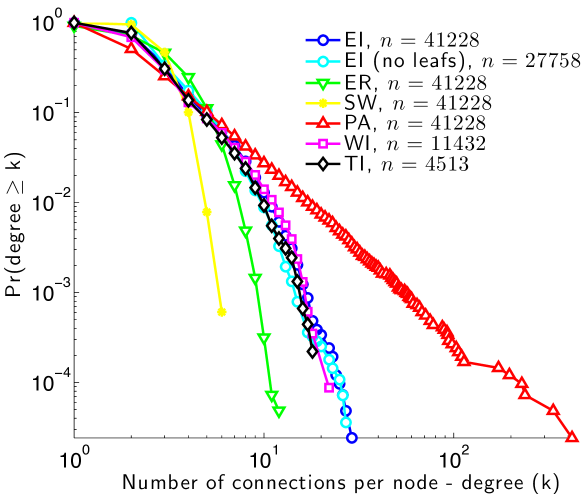
Figure 1: Cumulative degree distributions of the Eastern (EI), Western (WI) and Texas (TI) interconnections, along with degree distributions for synthetic networks—random (Erdős–R nyi, ER), small-world (SW) and preferential-attachment (PA)—sized to match EI: $|G_{EI}|=\{41228,52075\}$. Power networks have a heavy-tailed, but not power-law (scale-free) degree distribution.

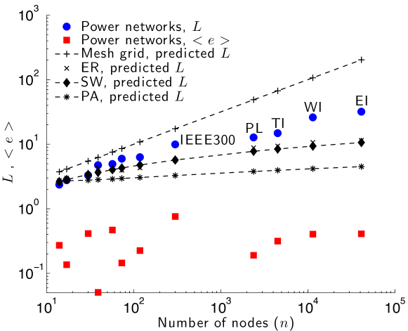
Figure 2: Characteristic path length ($L$) and average electrical distance ($\left\langle e\right\rangle$) of the power networks as a function of graph size, $n$. $L$ increases faster than $\ln n$ in the power networks, which indicates that the small-world model does not fit particularly well. PL is the test system “case2383wp” from Zimmerman:2011 . The smaller networks are standard IEEE test cases, also available from Zimmerman:2011 .

Tests of hypothesis 1 indicate that the degree distributions of the power networks do not match those of the synthetic networks in all but one case: the IEEE 300 network compared to a random graph. In Fig. 1, which shows the degree distributions for the large graphs, it is clear that high-degree nodes are more frequent than would be found in random graphs or small-world networks, but far less frequent than would be found in a similarly sized scale-free network. Hypothesis 1 can be rejected with high confidence.

The tests of hypothesis 2 show, with high confidence, that none of the North American power network degree distributions follow a power-law ($P<0.001$). The power-law exponents found ($\alpha=3.33$ to $\alpha=3.5$) are steeper than what would generally be considered notable power-law distributions Clauset:2009 . As expected the scale-free network fits well with a power-law degree distribution. These results lead us to conclude, with confidence, that power networks are not scale-free in topological structure.

The conjecture that power networks are small-world in structure requires some additional analysis. While the clustering coefficients of the power grids are less that those of the small-world graphs, $C$ is an order of magnitude higher in power grids than in random networks (table 1). To test whether the small-world model is a good model for power grids, we introduce a third hypothesis. Hypothesis 3 is that the characteristic path lengths of power grids increase with an upper bound of $L\leq\ln n$, which is argued in Watts:1998 and Boccaletti:2006 to be the limit for distances in small-world networks. Figure 2 compares the characteristic path lengths of several power networks with predicted values for $L$ from the small-world, scale-free, and random graph models. Path lengths in large power grids increase substantially faster than $\ln n$, which means that power grids fall somewhere between a regular grid, in which path lengths scale linearly with $n$ or $\sqrt{n}$, and a small-world network. Because $L>\ln n$ for all of the power networks of substantial size ($n>30$) hypothesis 3 can be safely rejected. Therefore, methods that are based on the assumption that power grids belong to the small-world family of networks (e.g., Fu:2010 ) may be misleading.

A number of other results in table 1 and Fig. 1 are notable. The small world networks had much higher clustering than the power networks, largely because the re-wiring probabilities ($p$) were chosen to keep distances similar to those found in the power networks, and were thus very small. That the power networks had a fairly high degree of clustering may be the result of geographic constraints that make very long-distance connections impractical in most cases. Also we find that power networks have a small, negative degree assortativity. In contrast, the small-world model shows a positive degree correlation, and, as expected, the preferential-attachment and random graph models show nearly zero assortativity. The negative assortativity in the power networks was found to result from substation buses with a large number of radial connections (typically distribution feeders). If the degree-1 “leaf nodes” are recursively removed the assortativity becomes very nearly zero. Upon recalculating the assortativity of EI, WI and TI after removing the leaf nodes, we find the following changes in assortativity: EI, from $r=-0.10$ to $-0.02$; WI, from $r=-0.08$ to $-0.01$; and TI, from $r=-0.09$ to $-0.02$.

III The electrical structure of power grids

While a thorough understanding of topological structure can be useful for some problems, such as producing synthetic power grids Wang:2010 , data about topological structure are not sufficient to describe the performance of power networks Hines:2010b . The connections between components in a power grid depend not only on its topology, but also on the the physical properties that govern voltages and currents.

One way to study connectivity between components in an electrical system is to look at the properties of sensitivity matrices. Sensitivity matrices for power systems, such as power transfer distribution factor matrices Bialek:1997 , measure the amount of influence that one component has on another. The complement of a sensitivity matrix is a distance matrix, which measures zero for component pairs that are perfectly connected, and large number for component pairs that have very little influence on one another. To our knowledge, the earliest work on electrical distances in power systems is in Lagonotte:1989 , in which the authors propose a distance metric based on voltage magnitude sensitivities and use this metric to divide a network into voltage control zones. They showed that the logarithmic voltage magnitude sensitivity in a power grid can qualify as a formal distance metric (see Appendix), under some conditions. Electrical distance measures have been applied to a number of reliability and economic power system problems Lu:1995 ; Hang:2000 ; Zhong:2004 .

The concept of “Resistance Distance,” as proposed in Klein:1993 , provides another method for computing electrical distances. Resistance distances give the effective resistance between points in a network of resistors. Here we extend the idea of resistance distance to represent the marginal effect of an active power transaction between buses $a$ and $b$ on voltage phase angle differences. Some transactions in a power system, such as those that occur over short, low impedance lines, have relatively minor effects on a network. Other transactions occur across high impedance paths, and thus result in large phase angle changes in the network. Large phase angle separations can expose instabilities in the system. Reference Dobson:2010b proposes the use of voltage phase angle differences between areas as a measure of stress in power networks. With this in mind we propose a distance metric based on the sensitivity between active power transfers and nodal phase angle differences.

To do so we start with a network of resistors with current injections at each node. Such a network can be described by a conductance matrix $\mathbf{G}$, such that the current injection at node $a$ is:

$$I_{a}=\sum_{b=1}^{n}g_{ab}V_{b}$$ (11)

When there are no connections to ground in the circuit, $\mathbf{G}$ has rank $n-1$, unless a voltage reference is specified. $\mathbf{G}$, thus defined acts as a Laplacian matrix for the resistive network. To get around the singularity of $\mathbf{G}$, we let node $r$ be a voltage reference node, with $V_{r}\triangleq 0$. The sub-matrix of $\mathbf{G}$ associated with the non-reference nodes ($\bar{r}$) is full-rank, therefore we can compute a sub-matrix $\mathbf{G}_{\bar{r}\bar{r}}^{-1}$, such that:

$$\mathbf{V}_{\bar{r}}=\mathbf{G}_{\bar{r}\bar{r}}^{-1}\mathbf{I}_{\bar{r}}.$$ (12)

If the diagonal element of $\mathbf{G}_{\bar{r}\bar{r}}^{-1}$ associated with node $a$ is $g_{a,a}^{-1}$, $g_{a,a}^{-1}$ indicates the change in voltage between nodes $a$ and $r$ as a result of a current injection at node $a$, which must be withdrawn from node $r$. This resistance distance gives the sensitivity between current injections and voltage differences. Therefore the resistance distance between $a$ and $r$ is equal to $g_{a,a}^{-1},\forall a$. To measure the distance between a pair of nodes $a$ and $b$, where $a\neq b\neq r$, one can evaluate:

$$e(a,b)=g_{a,a}^{-1}+g_{b,b}^{-1}-g_{a,b}^{-1}-g_{b,a}^{-1},$$ (13)

which gives the voltage difference between $a$ and $b$ after injecting 1 A at $a$ and withdrawing 1 A from $b$. In matrix form, where $\gamma\triangleq\mbox{diag}(\mathbf{G}_{\bar{r}\bar{r}}^{-1})$, the calculation proceeds efficiently as follows:

$$\mathbf{E}_{\bar{r}\bar{r}} = \mathbf{1}\gamma^{T}+\gamma\mathbf{1}^{T}-\mathbf{G}_{\bar{r}\bar{r}}^{-1}-[\mathbf{G}_{\bar{r}\bar{r}}^{-1}]^{T}$$ (14)

$$\mathbf{E}_{r,\bar{r}} = \gamma^{T}$$ (15)

$$\mathbf{E}_{\bar{r},r} = \gamma$$ (16)

where $\mathbf{E}_{\bar{r},r}$ refers to vector of non-reference elements in the reference column of the distance matrix. Resistance distance, thus defined, is proven to have the properties of a metric space in Klein:1993 .

To obtain sensitivities between power injections and phase angles, this definition requires some modification. To produce a real-valued distance metric, we start with the top half of the power flow Jacobian matrices:

$$\Delta\mathbf{P}=\left[\frac{\partial P}{\partial\theta}\right]\Delta\mathbf{\theta}+\left[\frac{\partial P}{\partial|V|}\right]\Delta|V|$$ (17)

If we assume that voltages are held constant ($\Delta|V|=0$), the matrix $[\partial P/\partial\theta]$ can be used to form a distance matrix. Under the dc power flow assumptions (nominal voltages, no resistive losses and small angle differences), $[\partial P/\partial\theta]$ is a Laplacian matrix that is analogous to $\mathbf{G}$. Even when these assumptions are relaxed, $[\partial P/\partial\theta]$ has most of the properties of a Laplacian. Applying (13) with $\mathbf{G}=[\partial P/\partial\theta]$ (with or without the dc approximations) results in a distance matrix ($\mathbf{E}$) that measures the incremental change in phase angle difference between nodes $a$ and $b$ ($\theta_{a}-\theta_{b}$) given an incremental average power transaction between nodes $a$ and $b$, assuming that voltage magnitudes are held constant. As in Lagonotte:1989 , we empirically found that $\mathbf{E}$, thus defined, satisfies the properties of a distance matrix so long as all series branch reactances are non-negative, as would be the case for nodes connected by a series capacitor (see Appendix).

Using this metric we can define a measure that is roughly analogous to node degree, but for a fully connected network with continuous weights for each node pair. To do so we measure the average distance from each node $a$ to other nodes in the system:

$$<e_{a}>=\sum_{b=1}^{n}\frac{e_{ab}}{n-1}$$ (18)

and invert it to obtain a measure of electrical centrality (modified from Hines:2008 ):

$$c_{a}=\frac{1}{<e_{a}>}.$$ (19)

The lower panel of Fig. 3 illustrates the electrical centrality of buses in the IEEE 300 bus system. In this system there are a group of buses with very high electrical connectivity, whereas the majority of buses have minimal centrality.

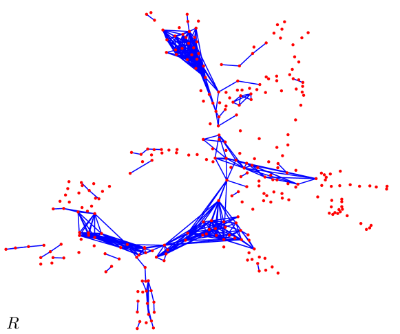
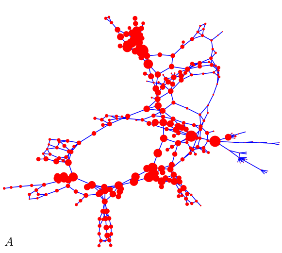
Figure 3: The upper panel shows a graphical representation of the electrical topology of the IEEE 300 bus system ($\mathbf{R}$), formed by replacing the 409 transmission branches with 409 shortest distance electrical links (the 409 smallest $e_{ij}$ such that $i>j$). The lower panel shows the topology ($\mathbf{A}$) of the 300 bus network with nodes drawn with sizes proportional to their electrical centrality (19).

Electrical distances are notably different than topological distances. Figure 4 shows that there is only a very weak correlation between electrical and topological distances ($\rho=0.24$ for $\left\langle e_{a}\right\rangle$ and $\left\langle d_{a}\right\rangle$). Many node pairs that are close topologically are distant in terms of electrical distance. It is notable that the correlation is stronger at the higher (500kV and 765kV) voltage levels where there is less diversity in branch impedances.

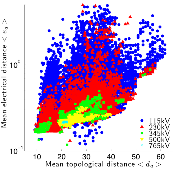
Figure 4: The mean topological and electrical (18) distances of buses, at different voltage levels, within the three North American power networks (EI, WI and TI). The average correlation between topological distance and electrical distance is low ($\rho=0.24$), however the correlation at the higher voltage levels ($\rho_{765}=0.43$, $\rho_{500}=0.65$) is higher.

Figure 5 compares the distribution of electrical and topological distances obtained from the EI, WI and TI models. The data indicate that topological distance distributions ($\mathbf{D}$) have exponential tails, whereas the electrical distance distributions ($\mathbf{E}$) have power-law tails.

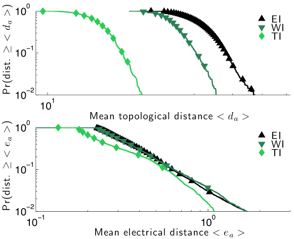
Figure 5: Complementary cumulative probability distributions for electrical and topological distances ($d_{ab}$ and $e_{ab}$) for the US Eastern, Western and Texas Interconnections. For the three distributions of topological distances, hypothesis 2 (see Section II.4) is rejected ($p<0.001$). For the two larger distributions of electrical distances (EI and WI), hypothesis 2 is not rejected and the estimates of $\alpha$ are: $\alpha_{EI}=3.49$ and $\alpha_{WI}=3.36$. For the distribution of electrical distances in TI, hypothesis 2 is rejected ($p<0.001$).

III.1 Representing electrical distances as an unweighted graph

The electrical distance matrix $\mathbf{E}$ describes the amount of connectivity between all node pairs in the system. Because Kirchhoff’s and Ohm’s laws produce comprehensive connectivity among all nodes in the system, the graph is weighted and fully connected (i.e., the network is an undirected graph with $n(n-1)$ weighted links). In order to compare this network with undirected, unweighted networks, we used the electrical distance matrix to produce an unweighted graph representation of the electrical structure of a power network. To do so, we kept the original $n$ nodes, but replaced the $m$ links with the $m$ smallest entries in the upper (or lower since $\mathbf{E}$ is symmetric) triangle of $\mathbf{E}$. Thus we created a graph of size $\{n,m\}$ with links representing strong electrical connections rather than direct physical connections. The adjacency matrix of this new graph ($\mathbf{R}$) is defined as follows:

$$\mathbf{R}:\,\begin{cases}r_{ab}=1&\forall e_{ab}<t\\ r_{ab}=0&\forall e_{ab}\geqslant t\end{cases}$$ (20)

where $t$ is a threshold adjusted to produce exactly $m$ links in the network. The upper panel of Fig. 3 shows the resulting electrical structure graph ($\mathbf{R}$) for the IEEE 300 bus test case. Comparison of the topological graph ($\mathbf{A}$ in Fig. 3) to the electrical one ($\mathbf{R}$ in Fig. 3) shows a stark contrast between the electrical and topological structure of the test system. A similar structural difference was found by comparing the topology and electrical structure of North American systems. Table 2 summarizes the calculated metrics for the Eastern Interconnection $\mathbf{R}$ matrix. Electrically speaking, a few nodes have a very high connectivity, whereas the vast majority of vertices in $\mathbf{R}$ have no connections. In this way, power systems share some properties with the scale-free network model; a few nodes have disproportionate influence on a large portion of the network. However, this is not to say that power systems will have all of the properties of scale-free networks (such as being highly vulnerable to directed attacks), since the response of power systems to disturbances depends on a wide variety of factors that are not captured in electrical distances.

The clustering coefficient of $\mathbf{R}$ is also high relative to the value obtained from the equivalent topological network. Both path lengths ($L$) and diameter ($d_{\max}$) are smaller in the electrical graph, indicating strong electrical connectedness within the core. The WI and TI electrical networks are highly disassortative ($r<0)$, whereas the EI system is electrically assortative ($r=0.33$).

Table 2: Topologically equivalent metrics for the reduced electrical distance matrices ($\mathbf{R}$).*

Network	EI ($\mathbf{R}$)	EI ($\mathbf{A}$)	WI ($\mathbf{R}$)	WI ($\mathbf{A}$)	TI ($\mathbf{R}$)	TI ($\mathbf{A}$)
Nodes**	41228 (56)	41228	11432 (8017)	11432	4513 (2769)	4513
Links	52075	52075	13734	13734	5532	5532
$<k>$	2.53	2.53	2.40	2.40	2.45	2.45
$\max(k)$	41171	29	3413	22	762	18
$C$	0.9996	0.068	0.9982	0.073	0.49	0.031
$L$	1.999	31.9	1.998	26.1	2.79	14.9
$d_{max}$	2	94	3	61	13	37
$r$	0.33	-0.10	-0.96	-0.08	-0.29	-0.09

* Metrics are calculated for the giant component.

** Numbers in parenthesis account for isolated nodes.

III.2 Electrical distance to load

The distance metric described by (12)-(14) gives sensitivities between arbitrary node pairs in a power network. We can refine this metric to focus on electrical distances from an arbitrary node to load nodes. This "electrical distance to load" measure describes the sensitivity of consumption nodes to perturbations at other locations in the network. In this section we determine the electrical distance to load of approximately 5600 buses within the US mid-Atlantic (PJM) portion of the EI model. From the electrical distance matrix, $\mathbf{E}$, we plot (Fig. 6) the amount of the total system load that is reachable at various electrical distances. Comparing this to a similar graph for topological distances illustrates the difference between the two. Topologically there are a few nodes that are within 1 link ($d_{ab}\leq 1$, or 5.3% of the topological diameter, $d_{\max}$) of about 2 GW of load, which is 1% of the total system load of 146.8 GW (lower panel of Fig. 6). Electrically, there are a few nodes that are within $e_{ab}\leq 0.011$ (0.5% of the electrical diameter, $e_{\max}$) of 40 GW (27%) of load. This indicates that a small number of nodes have a very high electrical influence on the system as a whole. Typically, these are high voltage buses (500kV and larger) that show very high electrical centrality.

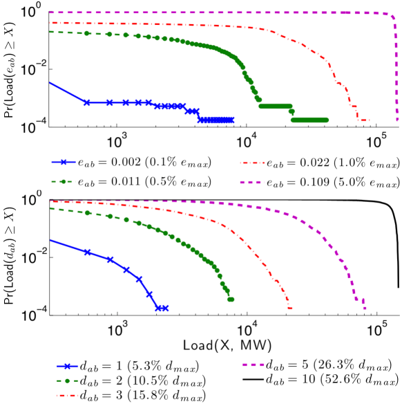
Figure 6: Electrical distances to loads for the PJM portion of the US Eastern Interconnect. The horizontal axis shows load, in MW. The vertical axis for the top panel shows the probability of a randomly selected node reaching $X$ MW of load within electrical distance $e_{ab}$. The lower panel shows the same result for topological distances. Comparing the purple line in the top figure (5% of $e_{max}$) with the blue line in the bottom figure (~5% of $d_{max}$) we see that it is possible to reach large amounts of load by traversing over short electrical distances, relative to the topological distances that one would need to cover to reach the same amount of load.

IV Conclusions

Power grids have been an appealing topic for network analysis in recent years, but the existing body of literature has produced some mixed results, particularly related to measuring the structure of power networks and connections between structure and performance. We have assessed the topological structure of the North American electric power network, and have compared it with a structural analysis based on a measure of “electrical distance," which measures network sensitivities. Electrical distance is more closely related to the physical laws governing behavior in electrical networks than topological distance or connectivity. In the appendix we show the conditions under which the proposed distance measure qualifies as a formal distance metric. Simpler impedance-based measures of electrical distance used elsewhere in the literature do not always meet the criteria for a proper distance metric.

Our analysis of the topological structure of the Eastern, Western and Texas Interconnects clearly suggests an exponential degree distribution rather than a power-law. We thus reject the conjecture that the observed power-law distribution in blackout sizes arises due to a power-law in the grid topology. Further, we observe significant differences between power-grid topologies and the topology of synthetic small-world networks. Distances between nodes increase much faster than the log of network size, and clustering is not as high as is found in true small-world networks. On a topological basis, we thus conclude that power grids are neither scale-free nor small-world in topological structure.

When we measure network structure based on electrical distance, however, we find a power-law distribution in electrical distances for all three Interconnects in the North American power network. It may be that this power-law distribution contributes to the empirically observed power-law distribution in large blackout sizes. Future work will seek to characterize the nature of this relationship. Also, we find that the correlation between electrical and topological distance is weak, though it increases for higher-voltage lines. When we look at the electrical distances between buses and loads in power networks, we find that a small number of nodes are tightly electrically connected to large percentages of load in the system, despite being relatively distant topologically. Since our electrical distance measure captures network sensitivities rather than physical connectivity, the observed heterogeneous structure suggests that perturbations (such as those caused by a volitional attack or changes in generator pricing) may have non-local effects more often than would be expected from the grid’s topological structure. Our work suggests that future endeavors to relate structure and performance in electrical networks should focus on characterizing network sensitivities rather than focusing narrowly on topological connectivity. Furthermore, this work suggests that circuit theory can be a useful tool in characterizing the connectivity and thus performance of complex networks.

Appendix. Conditions under which electrical distance qualifies as a formal distance measure

To qualify as a distance metric, a metric space $d(x,y)$ must map pairs of elements in a set in a way that describes the dissimilarity among any element ($x,y,z$), and must have the properties of non-negativity ($d(x,y)\geq 0$), symmetry ($d(x,y)=d(y,x)$), identity ($d(x,y)=0\Leftrightarrow x=y$) and the triangle inequality ($d(x,z)\leq d(x,y)+d(y,z)$) Rudin:1964 .

Equations (13)-(14) describe our measure of electrical distance $e(a,b)$, given a sensitivity matrix $\mathbf{G}$. Here we discuss the conditions under which $e(a,b)$ qualifies as a proper distance metric in some metric space. Following Rudin:1964 ; Klein:1993 , a distance metric $e(x,y)$ on an arbitrary metric space gives a measure of dissimilarity between arbitrary objects $x$ and $y$, and satisfies the following properties for all elements $a,b,c$:

• Symmetry: $e(a,b)=e(b,a)$

• Identity: $e(a,b)=0\Longleftrightarrow a=b$

• Non-Negativity: $e(a,b)\geq 0$

• Triangle Inequality: $e(a,b)+e(b,c)\geq e(a,c)$.

The discussion in this appendix will focus on the last of these properties, the triangle inequality. Lagonotte (Lagonotte:1989 ) found that an electrical distance measure related to voltages generally, but not always, obeyed the triangle inequality. We demonstrate a similar finding here for an analogous distance measure which is based upon real power sensitivities. Building on Lagonotte:1989 , we also characterize the conditions under which the triangle inequality will fail to hold for this electrical distance measure.

Recall, from the discussion surrounding (14), that the sensitivity matrix G is replaced with $[\partial\mathbf{P}/\partial\mathbf{\mathbf{\theta}}]$ from the power flow Jacobian. In the dc power flow model Stott:2009 , this sensitivity is simply equal to the system susceptance matrix B. For an arbitrary, connected three-node network, following (14), the electrical distance matrix E can be written as:

$$\left[\begin{array}[]{ccc}0&\frac{x_{12}(x_{13}+x_{23})}{x_{12}+x_{13}+x_{23}}&\frac{x_{13}(x_{12}+x_{23})}{x_{12}+x_{13}+x_{23}}\\ \frac{x_{12}(x_{13}+x_{23})}{x_{12}+x_{13}+x_{23}}&0&\frac{x_{23}(x_{12}+x_{13})}{x_{12}+x_{13}+x_{23}}\\ \frac{x_{13}(x_{12}+x_{23})}{x_{12}+x_{13}+x_{23}}&\frac{x_{23}(x_{12}+x_{13})}{x_{12}+x_{13}+x_{23}}&0\end{array}\right]$$ (21)

Applying the triangle inequality to (21), for each of the three triplets, leads to the following sufficient condition on the three reactances:

$$(x_{12}x_{23}\geq 0 \cap (x_{12}+x_{23}+x_{13})>0)\cup$$ (22)

$$(x_{12}x_{23}<0 \cap (x_{12}+x_{23}+x_{13})<0)$$

which is clearly satisfied for a strictly positive set of reactances. Figure 7 shows the volume in $x_{12},x_{13},x_{23}$ space where violations of the triangle inequality are observed, for all combinations of $x_{ab}\in[-1,1]$. Areas of the surface where

$$e(a,b)+e(b,c)-e(a,c)<0$$ (23)

were shaded, showing combinations of $x_{12},x_{13},x_{23}$ that yielded triangle inequality violations. Accordingly, if one or more of the branch reactances is less than zero, a violation may occur.

The extension of these analytical results to the ac power flow case remains for future work. However, in order to explore the triangle inequality conditions for a real power system we drew a random sample of $10^{6}$ node triplets from the Eastern Interconnect $\mathbf{E}$ matrix and tested against (23). This empirical evaluation showed that the triangle inequality holds for $99.81\%$ of the node triplets.

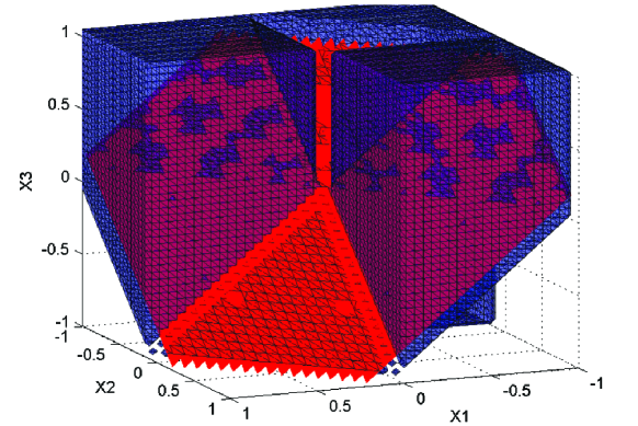
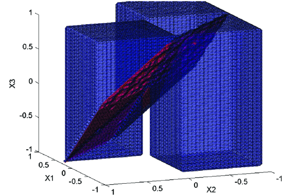
Figure 7: Illustration of the conditions under which three reactances ($x_{12},x_{23},x_{13})$ connecting a three-bus network satisfy the triangle inequality. Combinations that result in a triangle inequality violation are shaded. The two panels show the conditions from different perspectives. The red plane ($0=x1+x2+x3$) separates vertically the volumes corresponding to failure and success.

References

- (1) P. Erdös and A. Rényi, “On random graphs,” Publ. Math. Debrecen, vol. 6, pp. 290–297, 1959.
- (2) A. Barabási and R. Albert, “Emergence of scaling in random networks,” Science, vol. 286, no. 5439, pp. 509–512, 1999.
- (3) D. J. Watts and S. H. Strogatz, “Collective dynamics of ’small-world’ networks,” Nature, vol. 393, no. 6684, pp. 440–442, 1998.
- (4) S. Boccaletti, V. Latora, Y. Moreno, M. Chavez, and D. Hwang, “Complex networks: Structure and dynamics,” Physics reports, vol. 424, no. 4-5, pp. 175–308, 2006.
- (5) R. Albert, H. Jeong, and A. Barabási, “Error and attack tolerance of complex networks,” Nature, vol. 406, no. 6794, pp. 378–382, 2000.
- (6) X. Wang and G. Chen, “Synchronization in scale-free dynamical networks: robustness and fragility,” IEEE Transactions on Circuits and Systems I: Fundamental Theory and Applications, vol. 49, no. 1, pp. 54–62, 2002.
- (7) X. Li, X. Wang, and G. Chen, “Pinning a complex dynamical network to its equilibrium,” IEEE Transactions on Circuits and Systems I: Regular Papers, vol. 51, no. 10, pp. 2074–2087, 2004.
- (8) T. Chen, X. Liu, and W. Lu, “Pinning complex networks by a single controller,” IEEE Transactions on Circuits and Systems I: Regular Papers, vol. 54, no. 6, pp. 1317–1326, 2007.
- (9) F. Atay, T. Biyikoglu, and J. Jost, “Synchronization of networks with prescribed degree distributions,” IEEE Transactions on Circuits and Systems I: Regular Papers, vol. 53, no. 1, pp. 92–98, 2006.
- (10) C. Wu and L. Chua, “Synchronization in an array of linearly coupled dynamical systems,” IEEE Transactions on Circuits and Systems I: Fundamental Theory and Applications, vol. 42, no. 8, pp. 430–447, 1995.
- (11) C. Wu, “Synchronization in networks of nonlinear dynamical systems coupled via a directed graph,” Nonlinearity, vol. 18, p. 1057, 2005.
- (12) P. De Lellis, M. di Bernardo, and F. Garofalo, “Synchronization of complex networks through local adaptive coupling,” Chaos: An Interdisciplinary Journal of Nonlinear Science, vol. 18, no. 3, p. 037110, 2008.
- (13) P. De Lellis, M. di Bernardo, F. Garofalo, and M. Porfiri, “Evolution of complex networks via edge snapping,” IEEE Transactions on Circuits and Systems I: Regular Papers, vol. 57, no. 8, pp. 2132–2143, 2010.
- (14) F. Dorfler and F. Bullo, “Synchronization and transient stability in power networks and non-uniform kuramoto oscillators,” in American Control Conference (ACC), Baltimore, MD, USA. IEEE, 2010, pp. 930–937.
- (15) I. Dobson, B. Carreras, V. Lynch, and D. Newman, “Complex systems analysis of series of blackouts: Cascading failure, critical points, and self-organization,” Chaos: An Interdisciplinary Journal of Nonlinear Science, vol. 17, no. 2, p. 026103, 2007.
- (16) L. Amaral, A. Scala, M. Barthélémy, and H. Stanley, “Classes of small-world networks,” Proceedings of the National Academy of Sciences of the United States of America, vol. 97, no. 21, pp. 11 149–11 152, 2000.
- (17) R. Albert, I. Albert, and G. Nakarado, “Structural vulnerability of the north american power grid,” Physical Review E, vol. 69, no. 2, 2004.
- (18) P. Crucitti, V. Latora, and M. Marchiori, “A topological analysis of the italian electric power grid,” Physica A: Statistical Mechanics and its Applications, vol. 338, no. 1-2, pp. 92–97, 2004.
- (19) D. Chassin and C. Posse, “Evaluating north american electric grid reliaiblity using the barabasi-albert network model,” Physica A: Statistical Mechanics and its Applications, vol. 355, no. 2-4, pp. 667–677, 2005.
- (20) Å. Holmgren, “Using graph models to analyze the vulnerability of electric power networks,” Risk Analysis, vol. 26, no. 4, pp. 955–969, 2006.
- (21) R. Solé, M. Rosas-Casals, B. Corominas-Murtra, and S. Valverde, “Robustness of the european power grids under intentional attack,” Physical Review E, vol. 77, no. 2, p. 026102, 2008.
- (22) Z. Wang, A. Scaglione, and R. Thomas, “Generating statistically correct random topologies for testing smart grid communication and control networks,” IEEE Transactions on Smart Grid, vol. 1, no. 1, pp. 28–39, 2010.
- (23) J. Wang and L. Rong, “Cascade-based attack vulnerability on the us power grid,” Safety Science, 2009.
- (24) P. Hines, E. Cotilla-Sanchez, and S. Blumsack, “Do topological models provide good information about vulnerability in electric power networks?” Chaos: An Interdisciplinary Journal of Nonlinear Science, vol. 20, no. 3, p. 033122, 2010.
- (25) Z. Wang, A. Scaglione, and R. Thomas, “Electrical centrality measures for electric power grid vulnerability analysis,” in Proceedings of the 49th IEEE Conference on Decision and Control, Atlanta, Georgia. IEEE, 2010, pp. 5792–5797.
- (26) P. Hines and S. Blumsack, “A centrality measure for electrical networks,” in Proceedings of the 41st Hawaii International Conference on System Sciences, 2008.
- (27) P. Hines, S. Blumsack, E. Cotilla-Sanchez, and C. Barrows, “The topological and electrical structure of power grids,” in Proceedings of the 43rd Hawaii International Conference on System Sciences, 2010.
- (28) E. Bompard, R. Napoli, and F. Xue, “Analysis of structural vulnerabilities in power transmission grids,” International Journal of Critical Infrastructure Protection, vol. 2, no. 1-2, pp. 5–12, 2009.
- (29) S. Arianos, E. Bompard, A. Carbone, and F. Xue, “Power grids vulnerability: a complex network approach,” Chaos: An Interdisciplinary Journal of Nonlinear Science, vol. 19, no. 1, p. 013119, 2009.
- (30) S. Blumsack, L. Lave, and M. Ilic, “A quantitative analysis of the relationship between congestion and reliability in electric power networks,” Energy Journal, vol. 28, pp. 101–128, 2007.
- (31) D. Ming and H. Ping-ping, “Small-world topological model based vulnerability assessment algorithm for large-scale power grid,” Automation of Electric Power Systems, vol. 8, 2006.
- (32) V. Rosato, S. Bologna, and F. Tiriticco, “Topological properties of high-voltage electrical transmission networks,” Electric power systems research, vol. 77, no. 2, pp. 99–105, 2007.
- (33) L. Fu, W. Zhang, S. Xiao, Y. Li, and S. Guo, “Vulnerability assessment for power grid based on small-world topological model,” in Power and Energy Engineering Conference (APPEEC), 2010 Asia-Pacific, 2010.
- (34) M. Rosas-Casals, S. Valverde, and R. Solé, “Topological vulnerability of the european power grid under errors and attacks,” International Journal of Bifurcation and Chaos, vol. 17, no. 7, pp. 2465–2475, 2007.
- (35) PSTCA. (2007) Power Systems Test Case Archive, University of Washington, Electrical Engineering. [Online]. Available: http://www.ee.washington.edu/research/pstca/
- (36) R. Albert and A. Barabási, “Statistical mechanics of complex networks,” Reviews of modern physics, vol. 74, no. 1, p. 47, 2002.
- (37) M. Newman, “Assortative mixing in networks,” Physical Review Letters, vol. 89, no. 20, p. 208701, 2002.
- (38) ——, “Mixing patterns in networks,” Physical Review E, vol. 67, no. 2, p. 026126, 2003.
- (39) A. Clauset, C. Shalizi, and M. Newman, “Power-law distributions in empirical data,” SIAM Review, vol. 51, no. 4, pp. 661–703, 2009.
- (40) R. D. Zimmerman, C. E. Murillo-Sánchez, and R. J. Thomas, “MATPOWER: Steady-state operations, planning and analysis tools for power systems research and education,” IEEE Transactions on Power Systems, vol. 26, no. 1, pp. 12–19, 2011.
- (41) J. Bialek, “Topological generation and load distribution factors for supplement charge allocation in transmission open access,” IEEE Transactions on Power Systems, vol. 12, no. 3, pp. 1185–1193, 1997.
- (42) P. Lagonotte, J. Sabonnadiere, J. Leost, and J. Paul, “Structural analysis of the electrical system: application to secondary voltage control in france,” IEEE Transactions on Power Systems, vol. 4, no. 2, pp. 479–486, 1989.
- (43) Q. Lu and S. Brammer, “A new formulation of generator penalty factors,” IEEE Transactions on Power Systems, vol. 10, no. 2, pp. 990–994, 1995.
- (44) L. Hang, A. Bose, and V. Venkatasubramanian, “A fast voltage security assessment method using adaptive bounding,” IEEE Transactions on Power Systems, vol. 15, no. 3, pp. 1137–1141, 2000.
- (45) J. Zhong, E. Nobile, A. Bose, and K. Bhattacharya, “Localized reactive power markets using the concept of voltage control areas,” IEEE Transactions on Power Systems, vol. 19, no. 3, pp. 1555–1561, 2004.
- (46) D. Klein and M. Randic, “Resistance distance,” Journal of Mathematical Chemistry, vol. 12, pp. 81–95, 1993.
- (47) I. Dobson, M. Parashar, and C. Carter, “Combining phasor measurements to monitor cutset angles,” in Proc. of the 43rd Hawaii International Conference on System Sciences, Kauai, HI, 2010.
- (48) W. Rudin, Principles of mathematical analysis. McGraw-Hill New York, 1964, vol. 1976.
- (49) B. Stott, J. Jardim, and O. Alsac, “DC power flow revisited,” IEEE Transactions on Power Systems, vol. 24, no. 3, pp. 1290–1300, 2009.