Limb darkening in spherical stellar atmospheres

Abstract

Context. Stellar limb darkening, $I(\mu=\cos\theta)$, is an important constraint for microlensing, eclipsing binary, planetary transit, and interferometric observations, but is generally treated as a parameterized curve, such as a linear-plus-square-root law. Many analyses assume limb-darkening coefficients computed from model stellar atmospheres. However, previous studies, using $I(\mu)$ from plane-parallel models, have found that fits to the flux-normalized curves pass through a fixed point, a common $\mu$ location on the stellar disk, for all values of $T_{\mathrm{eff}}$, $\log g$ and wavelength.

Aims. We study this fixed $\mu$-point to determine if it is a property of the model stellar atmospheres or a property of the limb-darkening laws. Furthermore, we use this limb-darkening law as a tool to probe properties of stellar atmospheres for comparison to limb-darkening observations.

Methods. Intensities computed with plane-parallel and spherically-symmetric Atlas models (characterized by the three fundamental parameters $L_{\star}$, $M_{\star}$ and $R_{\star}$) are used to reexamine the existence of the fixed $\mu$-point for the parametrized curves.

Results. We find that the intensities from our spherical models do not have a fixed point, although the curves do have a minimum spread at a $\mu$-value similar to the parametrized curves. We also find that the parametrized curves have two fixed points, $\mu_{1}$ and $\mu_{2}$, although $\mu_{2}$ is so close to the edge of the disk that it is missed using plane-parallel atmospheres. We also find that the spherically-symmetric models appear to agree better with published microlensing observations relative to plane-parallel models.

Conclusions. The intensity fixed point results from the choice of the parametrization used to represent the limb darkening and from the correlation of the coefficients of the parametrization, which is a consequence of their dependence on the angular moments of the intensity. For spherical atmospheres, the coefficients depend on the three fundamental parameters of the atmospheres, meaning that limb-darkening laws contain information about stellar atmospheres. This suggests that limb-darkening parameterizations fit with spherically-symmetric model atmospheres are powerful tools for comparing to observations of red giant stars.

1 Introduction

The variation of the specific intensity over a star’s disk, commonly called limb darkening or center-to-limb variation, is an important function of the physical structure of a stellar atmosphere. Because it is difficult to observe limb darkening for stars other than the Sun, it is common to represent limb darkening by analytic expressions whose coefficients are determined by matching the $I_{\lambda}(\mu)$ from model stellar atmospheres. Here $\mu=\cos\theta$, where $\theta$ is the angle between the vertical direction at that point on the stellar disk and the direction toward the distant observer. The most basic form of the law is the linear version, depending on $\mu$ to the first power, such as

$$\frac{I_{\lambda}(\mu)}{I_{\lambda}(\mu=1)}=\mu,$$ (1)

or, more generally,

$$\frac{I_{\lambda}(\mu)}{I_{\lambda}(\mu=1)}=1-u(1-\mu).$$ (2)

Limb-darkening laws have subsequently become more complex by including terms with $\mu$, or its alternative $r=\sin\theta$, raised to higher integer powers as well as both $\sqrt{\mu}$ and $\log(\mu)$ terms (Claret, 2000; Howarth, 2010). In addition to minimizing the fit to the model’s $I_{\lambda}(\mu)$, the laws have also introduced various constraints, such as enforcing flux conservation at each observed wavelength. The intricacies of limb-darkening laws have increased as model stellar atmospheres have advanced.

Heyrovský (2000, 2003, 2007), motivated by the potential of gravitational microlensing to provide particularly detailed measurements of stellar limb darkening, investigated the optimum method of extracting limb darkening from the data. One curious feature that emerged from these studies is the existence of a fixed $\mu$ location on the stellar disk where the fits to the normalized model intensities have nearly the same value independent of wavelength or the model’s $T_{\mathrm{eff}}$ or $\log g$. This is true for both the principal-component analysis developed by Heyrovský (2003) and the more traditional linear limb-darkening law used by others.

Heyrovský (2003) used models computed with the Atlas12 code (Kurucz, 1996) to construct his fitting procedure. These models use detailed opacity sampling to include many tens of millions of spectral lines in the radiative transfer, but they still assumed plane-parallel geometry, even though Heyrovský (2003) targeted red giants with $T_{\mathrm{eff}}\leq 4000$ K and $\log g\leq 1.0$. These stellar parameters are exactly those where the assumption of plane-parallel geometry should break down. In the study by Claret & Hauschildt (2003), which did use the spherical models of Hauschildt et al. (1999), the focus was on models with $\log g\geq 3.5$, for which spherical extension is minimal. A broader study of limb darkening and the fixed $\mu$-point using spherically extended model atmospheres is clearly needed.

2 SAtlas model atmospheres

Lester & Neilson (2008) have developed the SAtlas code, a spherically extended version of Atlas. This code shares with Atlas the properties of static pressure structure, LTE populations and massive line blanketing represented by either opacity distribution functions or opacity sampling (the faster opacity distribution function version is used here). The spherical program differs from the plane-parallel Atlas by allowing the gravity to vary with radial position, and by computing the radiative transfer along rays through the atmosphere in the direction of the distant observer using the Rybicki (1971) version of the Feautrier (1964) method, which accounts for the radial variation of the angle between the vertical and the direction of the ray. The structure of the atmosphere is computed using a total of 81 rays whose angular spacing is determined by two factors. The first is the distribution of rays chosen to represent the “core” of the atmosphere, the region where the lower boundary condition for radiative transfer is the diffusion approximation. Lester & Neilson (2008) found that different distributions of the core rays had no effect on the structure of the atmosphere, and so elected to use equal spacings in $\mu$. The remainder of the rays are tangent to the atmospheric levels at the stellar radius perpendicular to the central ray toward the observer. These rays are projections of the radial spacing of the atmospheric levels, which is logarithmic in the Rosseland mean optical depth. Because this distribution of rays is set by calculating the structure of the atmosphere, it is not necessarily optimal for studying limb darkening. Therefore, after computing the structure of the atmosphere, the surface intensities are derived from the structure rays by cubic spline interpolation for any desired number of rays with any desired distribution over the disk. As Heyrovský (2007) has demonstrated, cubic spline provides an excellent interpolation method. We have created our surface intensities at 1000 points equally spaced over $0\leq\mu\leq 1$.

3 Fixed point of stellar limb-darkening laws

Heyrovský (2000) found the fixed point in the limb-darkening profiles of both the Sun and in plane-parallel Atlas models of red giants. Fields et al. (2003) found a similar fixed point in their analysis of a K3 giant using spherical Phoenix models, although they excluded the limb from their intensity analysis because the low intensity near the limb contributed almost nothing to the observations they were analyzing. Their truncation point ranged from $r=0.998$ for $\log g=3.5$, corresponding to $\mu=0.063$, to $r=0.88$ for $\log g=0.0$, corresponding to $\mu=0.475$. However, the truncation eliminated that part of the surface brightness that deviates most strongly from the plane-parallel model. Fields et al. (2003) stated that the fixed point is a generic feature of any single-parameter limb-darkening law that conserves flux. For example, if the limb darkening is represented as $f(\mu)\equiv I(\mu)/F=2[1+Ax(\mu)]$, the fixed point is $\mu_{\mathrm{fixed}}=f^{-1}[2\int_{0}^{1}f(\mu^{\prime})\mu^{\prime}\mathrm{d}\mu^{\prime}]$. Although they also state that the fixed point is not required by the two-parameter law they employed, they found a fixed point in the microlensing observations they were modeling using such a law.

To explore the parametrization more closely, we begin with the same two-parameter normalized limb-darkening function used by Fields et al. (2003),

$$\frac{I(\mu)}{2\mathcal{H}}=1-A\left(1-\frac{3}{2}\mu\right)-B\left(1-\frac{5}{4}\sqrt{\mu}\right),$$ (3)

where $\mathcal{H}$ in the Eddington flux, defined as

$$\mathcal{H}\equiv\frac{1}{2}\int_{-1}^{1}I(\mu)\mu\mathrm{d}\mu=\int_{0}^{1}I(\mu)\mu\mathrm{d}\mu.$$ (4)

A fixed point requires, for any two arbitrary models, that the intensity profiles satisfy

$$I_{1}(\mu_{0})=I_{2}(\mu_{0}),$$ (5)

or in terms of Eq. 3

$$1-A_{1}\left(1-\frac{3}{2}\mu_{0}\right)-B_{1}\left(1-\frac{5}{4}\sqrt{\mu_{0}}\right)=$$

$$\mbox{\hskip 42.67912pt}1-A_{2}\left(1-\frac{3}{2}\mu_{0}\right)-B_{2}\left(1-\frac{5}{4}\sqrt{\mu_{0}}\right).$$ (6)

For this to be true, $A$ and $B$ must be linearly dependent, $A=\alpha B+\beta$ or $A_{1}-A_{2}=\alpha(B_{1}-B_{2})$. Substituting this relation into Eq. 3 yields an equation for the fixed-point

$$\frac{3}{2}\alpha\mu_{0}+\frac{5}{4}\sqrt{\mu_{0}}-1-\alpha=0.$$ (7)

We need to verify that $A=f(B)$ and to understand the properties of the parameter $\alpha$.

Applying a general least-squares method to Eq. 3,

$$\chi^{2}=\sum_{i}^{N}\left[\frac{I(\mu_{i})}{2\mathcal{H}}-1+A\left(1-\frac{3}{2}\mu_{i}\right)+B\left(1-\frac{5}{4}\sqrt{\mu_{i}}\right)\right]^{2},$$ (8)

we determine the coefficients $A$ and $B$ from the constraint equations

$$\frac{\partial\chi^{2}}{\partial A} = \sum_{i}^{N}\left[\frac{I(\mu_{i})}{2\mathcal{H}}-1+A\left(1-\frac{3}{2}\mu_{i}\right)+B\left(1-\frac{5}{4}\sqrt{\mu_{i}}\right)\right]$$ (9)

$$\times\left(1-\frac{3}{2}\mu_{i}\right)=0$$

and

$$\frac{\partial\chi^{2}}{\partial B} = \sum_{i}^{N}\left[\frac{I(\mu_{i})}{2\mathcal{H}}-1+A\left(1-\frac{3}{2}\mu_{i}\right)+B\left(1-\frac{5}{4}\sqrt{\mu_{i}}\right)\right]$$ (10)

$$\times\left(1-\frac{5}{4}\sqrt{\mu_{i}}\right)=0.$$

Multiplying Eq. 9 and Eq. 10 by $\Delta\mu$ and then converting the summation to integration, $\int_{0}^{1}\mathrm{d}\mu$, we create the equations that determine $A$ and $B$,

$$\frac{J}{2\mathcal{H}}+\frac{1}{4}A+\frac{1}{6}B-1=0$$ (11)

and

$$-\frac{5}{4}\left[\frac{1}{2\mathcal{H}}\int_{0}^{1}I(\mu)\sqrt{\mu}\mathrm{d}\mu\right]+\frac{J}{2\mathcal{H}}+\frac{1}{6}A+\frac{11}{96}B-\frac{1}{6}=0,$$ (12)

where $J$ is the usual mean intensity. It is also useful to define an angular pseudo-moment of the intensity,

$$\mathcal{P}\equiv\int_{0}^{1}I(\mu)\sqrt{\mu}\mathrm{d}\mu,$$ (13)

which allows Eq. 12 to be written as

$$-\frac{5}{4}\left[\frac{\mathcal{P}}{2\mathcal{H}}\right]+\frac{J}{2\mathcal{H}}+\frac{1}{6}A+\frac{11}{96}B-\frac{1}{6}=0.$$ (14)

Both $J$ and $\mathcal{P}$ are determined by the properties of the model stellar atmosphere or the star whose observations are being fit by a limb-darkening law. Equation 11 and Eq. 12 clearly show that the coefficients $A$ and $B$ are uniquely determined by $J$ and $\mathcal{P}$. However, for $A$ and $B$ to be linearly dependent, that is $A=\alpha B+\beta$, $J$ and $\mathcal{P}$ must also be linearly related.

The relation of $J$ to $\mathcal{P}$ can be understood by following the discussion of the diffusion approximation in Mihalas (1978). This begins by representing the source function by a power series, which leads to the intensity being given by $I_{\nu}(\tau_{\nu},\mu)=\sum_{n=0}^{\infty}\mu^{n}\left[\mathrm{d}^{n}B_{\nu}(T)/\mathrm{d}\tau_{\nu}^{n}\right]$ (Mihalas 1978, Eq. 2-88). Using this expansion in the definitions of $J$ and $\mathcal{P}$, and keeping just the first-order term, gives the familiar results that $J_{\nu}\approx B_{\nu}$ and $K_{\nu}\approx B_{\nu}/3$ plus the additional result that $\mathcal{P}_{\nu}\approx 2B_{\nu}/3$. Eliminating $B_{\nu}$ between the $J_{\nu}$ and $\mathcal{P}_{\nu}$ expressions gives

$$\mathcal{P}_{\nu}=2J_{\nu}/3,$$ (15)

confirming the desired correlation. Of course, as the atmosphere thins out toward space the diffusion approximation becomes less accurate, but, as will be seen, the basic correlation of $\mathcal{P}$ and $J$ is still there.

Using Eq. 15 we can combine Eq. 11 and Eq. 12 to find that

$$A=-0.694B.$$ (16)

In terms of the notation used earlier, $\alpha=-0.694$ and $\beta=0$, or equivalently $\Delta A=-0.694\Delta B$. Using this value for $\alpha$ in Eq. 7 leads to the equation for the fixed point,

$$1.084\mu_{0}^{2}-0.925\mu_{0}+0.094=0.$$ (17)

This quadratic equation yields two fixed points, not one. The solutions are $\mu_{1}=0.736$, corresponding to $\theta_{1}=42.61^{\degr}$ and $r_{1}=0.677$, and $\mu_{2}=0.118$, corresponding to $\theta_{2}=83.22^{\degr}$ and $r_{2}=0.993$.

The results above used the diffusion approximation to establish the relationship between $J$ and $\mathcal{P}$. To generalize these results, we define a new variable, $\eta$, as

$$\eta\equiv\frac{\int I\sqrt{\mu}\mathrm{d}\mu}{J}=\frac{\mathcal{P}}{J}.$$ (18)

Note that $\eta$ is a generalization of the relation in Eq. 15. Using the definition of $\eta$, we replace the variable $\mathcal{P}$ in Eq. 14 by $\eta J$, and then Eq. 11 is used to eliminate the $J/2\mathcal{H}$ terms. The resulting equation is rearranged to the form $A=f(B)$, which is a linear equation of the same form as the previous equation for $A$, namely $A=\alpha B+\beta$. Comparing the two equations for $A$ we identify

$$\alpha=-\frac{(5\eta/4-1)/6+11/96}{(5\eta/4-1)/4+1/6}.$$ (19)

Equation 19 enables us to explore how $\alpha$ changes with $\eta$. In addition, because Eq 7 is a function of $\alpha$ only, we are also able to determine the dependence of the two fixed points, $\mu_{1}$ and $\mu_{2}$, on $\eta$. These dependencies are shown in Fig. 1. Because the value of $\eta$ can be set to values other than 2/3, the assumption of the diffusion approximation is no longer being used.

Figure 1: Top panel: dependence of the slope of the function $A=\alpha B+\beta$ on the variable $\eta=J^{-1}\int I\sqrt{\mu}\mathrm{d}\mu$. Bottom panel: variation of the fixed points with $\eta$.

Figure 1 shows that, except for $\eta\approx 0.267$, the value of $\alpha$ is in the narrow range $-0.72\lesssim\alpha\lesssim-0.68$, which leads to the fixed points being $0.72\lesssim\mu_{1}\lesssim 0.74$ and $0.08\lesssim\mu_{2}\lesssim 0.14$. The divergence of $\alpha$ to $\pm\infty$ as $\eta$ approaches $\approx 0.267$ is due to the denominator of Eq. 19 approaching zero as $\eta\rightarrow 4/15$. However, $\eta$ can never equal $4/15$. This is a consequence of the following inequalities, which are true because $\mu\leq 1$:

$$J=\int I\mathrm{d}\mu\geq\int I\sqrt{\mu}\mathrm{d}\mu\geq\int I\mu^{2}\mathrm{d}\mu=K.$$ (20)

Dividing through by $J$ this becomes

$$1\geq\eta\geq\frac{K}{J}.$$ (21)

Deep in the atmosphere, where the diffusion approximation holds, $K/J=1/3$. Moving toward the surface the atmosphere becomes more transparent and the radiation becomes less isotropic, with the consequence that $K/J>1/3$. As a result,

$$\eta\geq 1/3>4/15=0.267,$$ (22)

and the divergence cannot occur. Equation 19 can be used to set bounds on $\alpha$ by using the lower bound on $\eta$ from Eq. 22 and the upper bound on $\eta$ from Eq. 21. The result is $-5/6\leq\alpha\leq-15/22$. Using this range of $\alpha$ in Eq. 7, we find that the ranges for the fixed points are $0.708\leq\mu_{1}\leq 0.741$ and $0.025\leq\mu_{2}\leq 0.130$, which are consistent the values for $\mu_{1}$ and $\mu_{2}$ found previously. This indicates that the fixed points exist in the limb-darkening relations and are stable to differences in the intensity profile of the stellar atmosphere. It also suggests that the fixed points are not a result of a particular dominant opacity source. The only requirement is that $\eta>1/3$.

We verify this analytic result by computing a grid of Atlas plane-parallel model stellar atmospheres with $3000\ \mathrm{K}\leq T_{\mathrm{eff}}\leq 8000\ \mathrm{K}$ and $-2\leq\log g\leq 3$. For this grid of models, the mean value of $\eta$ in the $V-$band is $\bar{\eta}_{\mathrm{pp}}=0.716\pm 0.004$ which leads to $\alpha_{\mathrm{pp}}=0.691\pm 0.001$, $\mu_{1}=0.7375\pm 0.0002$ and $\mu_{2}=0.1200\pm 0.0003$. This is very similar to what is found assuming the diffusion approximation. The difference between the model $V-$band $\eta$ and the value of $\eta$ from the diffusion approximation is due to the fact that plane-parallel models do not enforce the diffusion approximation at all depths in the atmosphere. To determine the dependence on wavelength, we used the plane-parallel grid of atmospheres to determine the mean value and 1-$\sigma$ standard deviation of $\eta$, $\alpha$ and the two fixed points $\mu_{1}$ and $\mu_{2}$, with the results shown in Fig. 2. The values of the fixed points clearly do not vary significantly as a function of wavelength nor as a function of effective temperature and gravity. Furthermore, it must be noted that the value of $\eta$ approaches $2/3$ as $\lambda\rightarrow\infty$.

Figure 2: Wavelength dependence of the mean values of (a) the ratio of the pseudo-moment to the mean intensity, $\eta$, (b) the value of $\alpha$ that defines the fixed points, (c) the first and (d) second fixed point for the grid of plane-parallel Atlas model atmospheres. The error bars represent 1-$\sigma$ deviation from the mean.

These results can be generalized to show that the fixed point occurs in other limb-darkening laws, such as a quadratic law where $I/2\mathcal{H}=1-A(1-\mu)-B(1-2\mu^{2})$. Repeating the derivation above, the pseudo-moment, $\mathcal{P}$, is replaced by $K$, a higher angular moment of the intensity. Because the diffusion approximation analysis also yields a linear relation between $J$ and $K$, $J=3K$, we again find that $A=f(B)$. For a more general law, such as $I/2\mathcal{H}=1-A(1-\mu)-B[1-\frac{1}{2}(n+2)\mu^{n}]$, we would find a similar connection between the coefficients $A$ and $B$. We would even find fixed points for any law that is a combination of a linear term and any function that can be represented by a power-law series, such as $e^{\mu}$, similar to the limb-darkening law tested by Claret & Hauschildt (2003). Therefore, we conclude that the fixed points are a general property of this family of limb-darkening laws.

4 Limb darkening and SAtlas model atmospheres

To conduct a broader survey of limb darkening, we have computed several larger cubes of solar-composition model atmospheres, increasing the range of luminosity, mass and radius as well as using microturbulent velocities of 0, 2 and 4 km/s. The luminosities, masses and radii of these models cover a significant portion of the Hertzsprung-Russell diagram where stars have extended atmospheres, as shown in Fig. 3, which also shows the evolutionary tracks of Girardi et al. (2000) for comparison.

Figure 3: Models computed with the SAtlas code plotted over the stellar evolution tracks from Girardi et al. (2000).

Figure 4: Left panel: Limb darkening, characterized by the normalized surface intensity, $I(\mu)/2\mathcal{H}$, computed for the cube of 2102 model atmospheres for $v_{\mathrm{turb}}=2$ km/s for the $BVRI$ and $H$-bands. Right panel: Fit to these same intensities using the limb-darkening law $I(\mu)/2\mathcal{H}=1-A(1-\frac{3}{2}\mu)-B(1-\frac{5}{4}\sqrt{\mu})$ for the same wavebands.

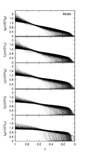
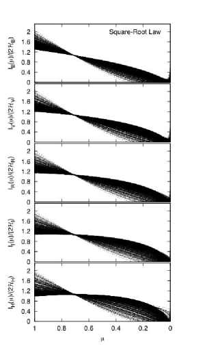
The number of models in each cube is large. For example, there were 2101 models in the cube with $v_{\mathrm{turb}}=2$ km/s and the cubes for the other values of $v_{\mathrm{turb}}$ have similar numbers of models. For each model in each cube we computed the intensity at 1000 equally spaced $\mu$ points at all wavelengths from the far ultraviolet to the far infrared; the results are shown in the left column of Fig. 4 for the $B,V,R,I$ and $H$-bands. These intensity curves have similar behavior as the Phoenix model atmosphere intensity curves that Orosz & Hauschildt (2000) studied. We also fit each of the model limb-darkening curves with the linear-plus-square-root limb darkening law given by Eq. 3, and this is shown in the right column of Fig. 4. Note that the $A$ and $B$ coefficients of this parametrization have been shown in Eq. 11 and Eq. 12 to be functions of $J$ and $\mathcal{P}$, not the structure of the intensity profile. The results for the $v_{\mathrm{turb}}=0$ and $4$ km/s cubes of models are very similar. This is not surprising; in the Atlas codes, the turbulent pressure is $P_{\rm{turb}}=\rho v_{\rm{turb}}^{2}$, indicating that the turbulent velocity has a similar effect on the temperature structure of a stellar atmosphere as the gravity, that is a change of turbulent velocity is equivalent to a change of gravity, similar to the discussion from Gustafsson et al. (2008) for the MARCS code. In terms of the best-fit relations, a change of turbulent velocity causes a small change for the coefficients in the same manner as a change in gravity for the same effective temperature and mass. Therefore, we can just explore the grid of models atmospheres for only one value of $v_{\rm{turb}}$. The cubes of models used in this survey cover a much wider range of atmospheric parameters than was used in the only previous investigation using spherical model stellar atmospheres (Claret & Hauschildt, 2003), which also truncated the profiles at the limb to achieve better fits.

The model intensities in the left column of Fig. 4 are always positive, but the intensities in some of the parametrized fits in the right column become slightly negative toward the limb. This does not happen for plane-parallel model atmospheres because the slope of the intensity profile ($\partial I/\partial\mu$ or $\partial I/\partial r$) has a constant sign. For example, using $\mu$ as the independent variable the slope of the intensity profile is always positive, varying from zero at the center of the disk to $\infty$ as $\mu\rightarrow 0$. For spherical atmospheres, the center-to-limb variation changes sign because of a slight inflection, which is apparent in the curves of the left column of Fig. 4. The more complex intensity profile and the use of an equal-weighting $\chi^{2}$-fit (i.e. the same number of $\mu$-points near the center as near the limb) leads to some slightly negative intensities in some best-fit relations.

Figure 4 shows that the actual limb darkening computed from the spherical models is more complex than the parametrized representation, and it is obvious that the analysis of specific observations that contain intensity information should be cautious about using the parametrized fits. Although fits to plane-parallel models appear to be very good, the models are less realistic physically than the spherical models. Therefore, using what seems like a well-fitting law may introduce hidden errors that could compromise the conclusions of the analysis. The quantities derived from observations of binary eclipses and planetary transits may be more uncertain than had been thought (see, for example, Knutson et al., 2007; Southworth et al., 2007; Southworth, 2008).

Using the same grid of spherical Atlas models used in Fig. 4, we computed the mean values and 1-$\sigma$ standard deviations of $\eta$, $\alpha$ and the fixed points as a function of wavelength. The results are shown in Fig. 5, which can be compared with the plane-parallel results shown in Fig. 2. There are two key differences between the plane-parallel and spherical models. The first is that the mean values of $\eta$ are larger for the spherical models, which leads to the differences between the mean values of $\alpha$ and the two fixed points. The second difference is that the standard deviation for $\eta$ as a function of wavelength is much larger for the spherical models than for the plane-parallel models. This suggests that $\eta$ varies much more as a function of effective temperature, gravity and mass. Clearly, the fixed point is much more constrained in plane-parallel model stellar atmospheres.

Figure 5: Wavelength dependence of the mean values of (a) the ratio of the pseudo-moment to the mean intensity, $\eta$, (b) the value of $\alpha$ that defines the fixed points, (c) the first and (d) second fixed point for the grid of spherically symmetric Atlas model atmospheres. The error bars represent 1-$\sigma$ deviation from the mean.

A specific example of an application of limb darkening to an observation is the analysis by Fields et al. (2003) of microlensing observations. In Fig. 6, we compare the $V$-band limb-darkening relations from our cube of spherical models with the $V$-band limb-darkening relation determined by Fields et al. (2003) from observations. It is clear that the Fields et al. (2003) $V$-band limb-darkening law agrees well with the limb-darkening from the spherical models, but, not as well with the plane-parallel models. Furthermore, although the curves for the model stellar atmospheres narrow to a waste rather than to a point, the location of minimum spread coincides with the location of the observed $\mu$-position in the $V$-band limb-darkening relation within the uncertainty of the observed coefficients. Even though the uncertainty of limb-darkening relations from microlensing observations is large, these results suggest that the Fields et al. (2003) limb-darkening observations are probing the extended the atmosphere of the lensed red giant star.

Figure 6: Comparison of the $V$-band limb-darkening relation determined by Fields et al. (2003) from observations (black dashed curves with errorbars) with the limb-darkening relations computed from SAtlas model stellar atmospheres (red solid curves) and relations computed from Atlas model stellar atmospheres (blue dotted curves), represented using the same linear-plus-square-root law. The insert shows a magnified view of the region of the fixed $\mu$-point.

Figure 7: Red plus symbols represent the limb-darkening coefficients $A$ and $B$ computed from SAtlas model intensity profiles for the $V$, $I$, and $H$-bands, and green open squares represent the coefficients computed with plane-parallel Atlas models. The box in each plot shows the range of the coefficients derived from microlensing observations by Fields et al. (2003).

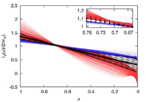
We conclude that the parametrized laws, although more simplified than the computed limb-darkening curves, are useful for understanding how limb darkening depends on the fundamental properties of the stellar atmosphere.

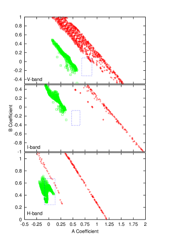
To explore further the information content of the limb darkening, we recall that Eq. 16 showed that the coefficients $A$ and $B$ of the parametrization are linearly correlated. In Fig. 7 we plot the limb-darkening coefficients $A$ and $B$ for the $V$, $I$, and $H$-bands computed with both the plane-parallel Atlas and the spherical SAtlas models. For each wavelength the error box shows the range of $A$ and $B$ found by Fields et al. (2003) from their observations. For the $V$-band, the spherical limb-darkening coefficients overlap with the observed fit, but the plane-parallel coefficients do not, while for $H$-band both plane-parallel and spherical models agree with observations. The microlensing observations at the longer wavelength might not be sensitive enough to probe the low intensity limb of the star, making the star appear consistent with limb-darkening of the plane-parallel model atmospheres. In the $I$-band neither set of models agree with the observations, but the $I$-band data provide a weak constraint. As Fields et al. (2003) noted, the $I$-band time-series microlensing observations were a composite from multiple sites, and removing data from any one site changed the results significantly.

Figure 8: Left: As a function of surface gravity, the top panel shows the value of the primary fixed point, $\mu_{1}$, for the linear plus square root parametrization, for spherical atmospheres of varying effective temperature. The bottom panel shows the dependence of the normalized V-band intensity of the fixed point. Red fiilled circles are $T_{\mathrm{eff}}=3000$ K, green open squares 4000 K, blue open circles 5000 K, magenta downward pointing triangles 6000 K and pale blue upward pointing triangles are 7000 K. The black crosses show the behavior of the fixed point from the grid of plane-parallel model atmospheres for comparison Right: As a function of effective temperature, the top panel shows the fixed point, $\mu_{1}$, and the bottom panel shows the dependence of the V-band intensity of the fixed point. Red triangles represents models with $\log\leavevmode\nobreak\ g=0$, green squares $\log\leavevmode\nobreak\ g=1$, and blue circles are $\log\leavevmode\nobreak\ g=2$. Again, black crosses represent the fixed point from plane-parallel model atmospheres.

In the $V$-band, the limb-darkening coefficients from 15 model atmospheres fall within the observational box. These models have $\log\leavevmode\nobreak\ g=2.25-3$ and $T_{\mathrm{eff}}=3400-3600$ K. For the $H$-band data there are four models within the observational box; these have same range of gravities but are slightly cooler, $T_{\mathrm{eff}}=3000-3100$ K. It is interesting that the models that agree with the observations are those with gravities that are consistent with the results of Fields et al. (2003) and An et al. (2002). This suggests that observations using the limb-darkening parametrization can probe the spherical extension of stellar atmosphere via the fixed point, $\mu_{1}$, and potentially probe the fundamental parameters of stars via the limb-darkening coefficients.

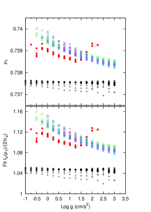
Using a cube of models with a given value of $v_{\mathrm{turb}}$, we examine the dependence of the primary fixed point, $\mu_{1}$, on the effective temperature and surface gravity. Note again that there are three basic parameters characterizing the spherical atmospheres: $L_{\star}$, $M_{\star}$ and $R_{\star}$. This means that values of $T_{\mathrm{eff}}$ and $\log g$ are degenerate, but they are easier to show on a two-dimensional surface. In the top left panel of Fig. 8 we plot the value of the primary fixed point, $\mu_{1}$, as a function of $\log g$. At each value of $\log g$ there are values of $T_{\mathrm{eff}}$ ranging from 3000 to 7000 K, although there can be multiple values because of the parameter degeneracy. In the bottom left panel of Fig. 8 we plot $I_{\mathrm{V}}(\mu_{1})/2\mathcal{H}_{\mathrm{V}}$, the normalized intensity of the fixed point in the $V$-band. For each surface gravity the values of $\mu_{1}$ and the normalized intensity at the fixed point both show a steady progression as $T_{\mathrm{eff}}$ changes, except for $T_{\mathrm{eff}}=3000$ K. We suspect that the behavior for $T_{\mathrm{eff}}=3000$ K is due to a change in the dominant opacity source for our coolest models, possibly water vapor. Models with $T_{\mathrm{eff}}>3000$ K have H^- as the dominant continuous opacity, but in the coolest models there are fewer free electrons available to form H^-, and the formation of H₂ reduces the pool of hydrogen atoms. We also plot the fixed point and intensity at the fixed point from plane-parallel model atmospheres for comparison. It is clear that the fixed point from fits to plane-parallel models varies much less than fits to spherical models.

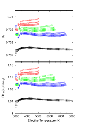
On the right side of Fig. 8 we reverse the parameters and plot the dependence of the primary fixed point and the normalized intensity of the fixed point as a function of $T_{\mathrm{eff}}$. At each value of the effective temperature, the values of $\log g$ are 0, 1 and 2 in cgs units. In the top right panel of Fig. 8 we see that there is essentially no variation of the value of $\mu_{1}$ with $T_{\mathrm{eff}}$ for all three surface gravities until the lowest effective temperature is reached. There is an obvious displacement of the value of $\mu_{1}$ for each gravity and also a spread in $\mu_{1}$ because of parameter degeneracy. However, for $T_{\mathrm{eff}}\leq 3500$ K the value of $\mu_{1}$ drops for all surface gravities. The bottom right panel shows that the normalized $V$-band intensity of the fixed point shows a similar behavior. For $T_{\mathrm{eff}}>3500$ K there is little variation with $T_{\mathrm{eff}}$, but there is an offset and a spread that depends on the surface gravity. Cooler than 3500 K the value of the normalized intensity drops noticeably.

It is clear that the fixed point $\mu_{1}$ and the intensity at the fixed point $I(\mu_{1})/2\mathcal{H}$ are functions of gravity and effective temperature for spherically-symmetric models and are roughly constant for plane-parallel model atmospheres. This indicates that the best-fit coefficients of the limb-darkening law vary mostly because of the geometry of the model atmosphere. A spherical model atmosphere predicts a smaller intensity near the limb of the stellar disk relative to a plane-parallel model with the same effective temperature and gravity. To predict the same emergent flux, the intensity must be larger at the center of the disk, hence the temperature at the base of the atmosphere must also be larger for the spherical model. Therefore, the temperature structure of the atmosphere also varies. However, this is a secondary effect and the geometry of the atmosphere is most important in determining the value of the $\mu_{1}$ and $I(\mu_{1})/2\mathcal{H}$. The geometry of spherical models leads to smaller values of the pseudo-moment and the mean intensity because the intensity is more centrally concentrated. This suggests that $\mu_{1}$ and $I(\mu_{1})/2\mathcal{H}$ depend on the atmospheric extension. We will explore how the fixed point and intensity relate to the extension and fundamental stellar properties in greater detail in a future article.

5 Conclusions

We have explored limb darkening using large cubes of spherical stellar atmospheres spanning the parameters $L_{\star}$, $M_{\star}$ and $R_{\star}$ covering the cool, luminous quadrant of the Hertzsprung-Russell diagrams (Fig. 3). These models have also used three different values of the microturbulent velocity. For each model, the center-to-limb variation of the surface intensity has been calculated at 1000 equally spaced $\mu$ values spanning the range from 1 to 0 for every wavelength used to compute the model structure.

Parametrizing the center-to-limb variation with a flux-conserving linear-plus-square-root limb-darkening law, we confirm the findings of Heyrovský (2000) and Fields et al. (2003) that there is a fixed $\mu_{1}$ point through which all the intensity curves pass. However, when we plot the surface intensities directly, without using a fitting law, there is no fixed point, although the distribution of curves does narrow to a waist close to the same value of $\mu_{1}$ (Fig. 4).

The apparent fixed point is a result of the least-squares fitting procedure where the two parameters of the law are dependent on two properties of the stellar atmosphere, the mean intensity, $J$, and the pseudo-moment, $\int I\sqrt{\mu}\mathrm{d}\mu$. For the temperature range $4000-8000$ K, the mean intensity is correlated with the pseudo-moment, which means that the two coefficients are also correlated, leading to the existence of the fixed point.

The lack of a well-defined fixed point in the surface intensity distribution for spherical model atmospheres suggests that the three fundamental parameters of the atmospheres affect the limb darkening in a way that is not encountered in the two-parameter plane parallel atmospheres.