Characterization of vector diffraction-free beams

Abstract

It is observed that a constant unit vector denoted by $\mathbf{I}$ is needed to characterize a complete orthonormal set of vector diffraction-free beams. The previously found diffraction-free beams are shown to be included as special cases. The $\mathbf{I}$-dependence of the longitudinal component of diffraction-free beams is also discussed.

Any light beams other than plane waves are usually diffractively spreading in propagation. But it was predicted Durnin and then experimentally observed Durnin-ME that there exists a kind of $J_{0}$ “scalar” mode the intensity of which is free of diffraction. With the understanding Davis-P ; Davis-P2 ; Jordan ; Hall of the so-called cylindrical-vector beams Youngworth-B , it was found Bouchal-O that there also exists a kind of cylindrical-vector modes the intensity and vectorial structure of which is free of diffraction. Those two kinds of diffraction-free beams share the same property that all the wavevectors of the constituent plane waves lie on the surface of a cone.

The “scalar” beam is in fact a uniformly polarized beam that is valid only in the paraxial limit Lax-LM . The cylindrical-vector beam is such a beam the direction of whose electric vector is rotationally symmetric about its propagation axis. The problems with which we are concerned here are whether there exist other kinds of diffraction-free beams and whether we can find a precise scheme to distinguish between different diffraction-free beams. Recently, a characteristic denoted by a constant unit vector $\mathbf{I}$ was demonstrated Li to convey the vectorial nature of a light beam. The uniformly polarized beam has a characteristic vector that is perpendicular to the propagation direction. The cylindrical-vector beam has a characteristic vector that is parallel to the propagation direction. The purpose of this paper is to classify the vector diffraction-free beams with the $\mathbf{I}$ and to explore the dependence of their vectorial property on the $\mathbf{I}$. It will be shown that the $\mathbf{I}$ is a continuous index to characterize a complete orthonormal set of vector diffraction-free beams. Different $\mathbf{I}$’s represent different complete orthonormal sets of vector diffraction-free beams.

For simplicity, only monochromatic light beams are considered. We do not solve the vector Helmholtz equation together with the transversality condition. Instead, we directly make use of the transversality condition to write out the integral expression for the diffraction-free beams, because such an approach explicitly demonstrates Li the necessity of introducing the characteristic vector. As we know, the electric vector $\mathbf{f}(\vartheta,\varphi)$ of a monochromatic light beam in the momentum representation can be factorized Akhiezer into a polarization vector $\mathbf{e}(\vartheta,\varphi)$ and a scalar magnitude $f(\vartheta,\varphi)$ as

$$\mathbf{f}(\vartheta,\varphi)=\mathbf{e}(\vartheta,\varphi)f(\vartheta,\varphi),$$ (1)

where $\vartheta$ and $\varphi$ are the polar and azimuthal angles of the wavevector $\mathbf{k}$, respectively, in the spherical polar coordinates. The transversality condition means that the polarization vector $\mathbf{e}$ is perpendicular to the wavevector and can be expanded in terms of a set of base polarization vectors as

$$\mathbf{e}(\vartheta,\varphi;\mathbf{I})=\alpha_{1}\mathbf{e}_{1}(\vartheta,\varphi;\mathbf{I})+\alpha_{2}\mathbf{e}_{2}(\vartheta,\varphi;\mathbf{I}),$$ (2)

where the base vectors $\mathbf{e}_{1}$ and $\mathbf{e}_{2}$ are defined Li by means of a constant unit vector $\mathbf{I}$ as

$$\mathbf{e}_{1}(\vartheta,\varphi;\mathbf{I})=\mathbf{e}_{2}\times\frac{\mathbf{k}}{k},\hskip 5.0pt\mathbf{e}_{2}(\vartheta,\varphi;\mathbf{I})=\frac{\mathbf{k}\times\mathbf{I}}{|\mathbf{k}\times\mathbf{I}|},$$ (3)

$\alpha_{1}$ and $\alpha_{2}$ are complex constants satisfying $|\alpha_{1}|^{2}+|\alpha_{2}|^{2}=1$, and the dependence of $\mathbf{e}$ on the $\mathbf{I}$ is explicitly shown. In addition, the scalar magnitude $f(\vartheta,\varphi)$ for an arbitrary monochromatic beam of wave number $k$ can be expanded in terms of the following complete orthonormal set of scalar functions,

$$f_{k_{z}l}(\vartheta,\varphi)=\frac{\delta(\vartheta-\vartheta_{0})}{i^{l}\sqrt{2\pi k}\sin\vartheta_{0}}e^{il\varphi},\hskip 5.0ptl=0,\pm 1,\pm 2...$$ (4)

where the longitudinal component of the wavevector, $k_{z}=k\cos\vartheta_{0}$, is chosen to be one of the indices. The orthonormality property assumes the form

$$\int f^{\ast}_{k^{\prime}_{z}l^{\prime}}f_{k_{z}l}\sin\vartheta d\vartheta d\varphi=\delta_{l^{\prime}l}\delta(k^{\prime}_{z}-k_{z}),$$ (5)

where $k^{\prime}_{z}=k\cos\vartheta^{\prime}_{0}$. The electric vector of the beam in the position representation that is associated with the momentum-representation electric vector (1) is given by

$$\mathbf{E}(\mathbf{I})=\frac{1}{2\pi}\int\mathbf{f}(\vartheta,\varphi;\mathbf{I})e^{i\mathbf{k}\cdot\mathbf{x}}\sin\vartheta d\vartheta d\varphi.$$ (6)

From the complete orthonormal set of base vectors (3) and the complete orthonormal set of scalar functions (4), one readily writes down the following complete orthonormal set of vector functions,

$$\mathbf{f}_{\sigma,k_{z}l}(\vartheta,\varphi;\mathbf{I})=\mathbf{e}_{\sigma}(\vartheta,\varphi;\mathbf{I})f_{k_{z}l}(\vartheta,\varphi),$$ (7)

where $\sigma=1,2$. They satisfy the relation

$$\int\mathbf{f}^{\ast}_{\sigma^{\prime},k^{\prime}_{z}l^{\prime}}\cdot\mathbf{f}_{\sigma,k_{z}l}\sin\vartheta d\vartheta d\varphi=\delta_{\sigma^{\prime}\sigma}\delta_{l^{\prime}l}\delta(k^{\prime}_{z}-k_{z}).$$ (8)

Now we are in a position to show that the beams associated with the electric vector (7) in the momentum representation are diffraction-free. Substituting Eqs. (7) and (4) into Eq. (6) and performing the integration over $\vartheta$, one finds

$$\mathbf{E}_{\sigma,k_{z}l}(\mathbf{I})=\frac{e^{ik_{z}z}}{2\pi i^{l}}\int\mathbf{e}_{\sigma}(\vartheta_{0},\varphi;\mathbf{I})e^{il\varphi}e^{i\kappa\rho\cos(\phi-\varphi)}d\varphi,$$ (9)

where $\kappa=k\sin\vartheta_{0}$ is the transverse component of the wavevector, the position vector $\mathbf{x}$ is expressed as $\mathbf{x}=\mathbf{e}_{x}\rho\cos\phi+\mathbf{e}_{y}\rho\sin\phi+\mathbf{e}_{z}z$ in the circular cylindrical coordinates, and an irrelevant factor $1/\sqrt{2\pi k}$ is omitted. The beams represented by Eq. (9) are indeed diffraction-free, because only the propagation factor $\exp(ik_{z}z)$ depends on the $z$ coordinate. Eqs. (7) and (4) show that all the wavevectors in these diffraction-free beams lie on the surface of a cone, the cone angle of which is $\vartheta_{0}$.

The index $\sigma$ in Eq. (7) as well as Eq. (9) expresses the restriction imposed by the transversality condition. Although it requires that the base vectors $\mathbf{e}_{\sigma}$ be perpendicular to the wavevector, the transversality condition itself is not able to prescribe Li the exact relations of $\mathbf{e}_{\sigma}$ with the wavevector. Those relations are determined here by the unit vector $\mathbf{I}$ in Eqs. (3). This shows that one needs to use $\sigma$ as well as $\mathbf{I}$ together to characterize the vectorial nature of a vector diffraction-free beam. Since every specified $\mathbf{I}$ defines a complete orthonormal set of vector diffraction-free beams as is explicitly indicated in Eq. (9), the $\mathbf{I}$ turns out to be an index to characterize such a complete orthonormal set. It is noted that the $\mathbf{I}$ is always perpendicular to $\mathbf{E}_{2,k_{z}l}$.

Next, let us show how the previously found diffraction-free beams can be obtained from Eq. (9). To this end, we let $\mathbf{I}$ lie in the $xoz$ plane,

$$\mathbf{I}=\mathbf{e}_{x}\sin\Theta+\mathbf{e}_{z}\cos\Theta,$$ (10)

paying our attention only to the effect of its polar angle $\Theta$. This is because the angular-spectrum function (4) is rotationally symmetric about the $z$ axis. Rotation of $\mathbf{I}$ about the $z$ axis amounts to a rotation of the diffraction-free beam in the same way. In the first place, we assume that the $\mathbf{I}$ is perpendicular to the $z$ axis, $\Theta=\frac{\pi}{2}$. In this case, one finds from Eq. (3)

$$\mathbf{e}_{1}= \mathbf{e}_{x}(1-\sin^{2}\vartheta\cos^{2}\varphi)^{1/2}$$

$$-\frac{\mathbf{e}_{y}\sin\vartheta\sin\varphi+\mathbf{e}_{z}\cos\vartheta}{(1-\sin^{2}\vartheta\cos^{2}\varphi)^{1/2}}\sin\vartheta\cos\varphi,$$ (11a)

$$\mathbf{e}_{2}= \frac{\mathbf{e}_{y}\cos\vartheta-\mathbf{e}_{z}\sin\vartheta\sin\varphi}{(1-\sin^{2}\vartheta\cos^{2}\varphi)^{1/2}}.$$ (11b)

Both of them have longitudinal components. Here $\sin\vartheta$ corresponds to the small number $f$ discussed in Ref. Lax-LM when the wavevector cone is very close to the $z$ axis. To the zeroth-order paraxial approximation, one has $\mathbf{e}_{1}\approx\mathbf{e}_{x}$ and $\mathbf{e}_{2}\approx\mathbf{e}_{y}$. Substituting them into Eq. (9), one obtains

$$\mathbf{E}_{1,k_{z}l}=\mathbf{e}_{x}J_{l}e^{il\phi}e^{ik_{z}z},\hskip 5.0pt\mathbf{E}_{2,k_{z}l}=\mathbf{e}_{y}J_{l}e^{il\phi}e^{ik_{z}z},$$ (12)

where $J_{l}=J_{l}(\kappa\rho)$ is the $l$th-order Bessel function of the first kind. The case of $l=0$ leads to the uniformly polarized $J_{0}$ diffraction-free beam found in Refs. Durnin ; Durnin-ME . In the second place, we assume that the $\mathbf{I}$ is parallel to the $z$ axis, $\Theta=0$. In this case, one has $\mathbf{e}_{1}=-\mathbf{e}_{\kappa}\cos\vartheta+\mathbf{e}_{z}\sin\vartheta$ and $\mathbf{e}_{2}=-\mathbf{e}_{\varphi}$. Upon substituting into Eq. (9), one gets

$$\mathbf{E}_{1,k_{z}l}= \frac{i}{2}[(\mathbf{e}_{\rho}+i\mathbf{e}_{\phi})J_{l-1}-(\mathbf{e}_{\rho}-i\mathbf{e}_{\phi})J_{l+1}]$$

$$\times\cos\vartheta_{0}e^{il\phi}e^{ik_{z}z}+\mathbf{e}_{z}J_{l}\sin\vartheta_{0}e^{il\phi}e^{ik_{z}z},$$ (13a)

$$\mathbf{E}_{2,k_{z}l}= \frac{1}{2}[(\mathbf{e}_{\rho}+i\mathbf{e}_{\phi})J_{l-1}+(\mathbf{e}_{\rho}-i\mathbf{e}_{\phi})J_{l+1}]$$

$$\times e^{il\phi}e^{ik_{z}z}.$$ (13b)

Here $\mathbf{E}_{1,k_{z}l}$ and $\mathbf{E}_{2,k_{z}l}$ are exactly the vector solutions $\mathbf{N}_{n}$ and $\mathbf{M}_{n}$, respectively, found in Ref. Bouchal-O . In fact, the authors of Ref. Bouchal-O also made use of a constant vector. Unfortunately, they just assumed that vector to be the unit vector in the $z$ direction.

In Eq. (9), we chose the linearly-polarized base vectors $\mathbf{e}_{\sigma}$ for the vector diffraction-free beams. If we choose the circularly-polarized base vectors, $\mathbf{e}_{\pm}=\frac{1}{\sqrt{2}}(\mathbf{e}_{1}\pm i\mathbf{e}_{2})$, and let the $\mathbf{I}$ lie along the $z$ axis, we will arrive at a complete orthonormal set of vector diffraction-free beams that was found in Ref. Enk-N .

At last, let us have a look at the effect of $\mathbf{I}$ on the vectorial property of the diffraction-free beams by examining the $\mathbf{I}$-dependence of their longitudinal components. For this purpose, we take $l=2$ as an example. With the $\mathbf{I}$ being given by Eq. (10), we have for the $z$ components of $\mathbf{e}_{1}$ and $\mathbf{e}_{2}$, respectively,

$$e_{1}^{z} =\frac{\sin^{2}\vartheta\cos\Theta-\sin\vartheta\cos\vartheta\cos\varphi\sin\Theta}{[1-(\sin\vartheta\cos\varphi\sin\Theta+\cos\vartheta\cos\Theta)^{2}]^{1/2}},$$ (14a)

$$e_{2}^{z} =-\frac{\sin\vartheta\sin\varphi\sin\Theta}{[1-(\sin\vartheta\cos\varphi\sin\Theta+\cos\vartheta\cos\Theta)^{2}]^{1/2}}.$$ (14b)

The $z$ components of $\mathbf{E}_{\sigma,k_{z}2}$ are thus given by

$$E^{z}_{\sigma,k_{z}2}=-\frac{e^{ik_{z}z}}{2\pi}\int e_{\sigma 0}^{z}e^{2i\varphi}e^{i\kappa\rho\cos(\phi-\varphi)}d\varphi,$$ (15)

where $e_{\sigma 0}^{z}=e_{\sigma}^{z}|_{\vartheta=\vartheta_{0}}$. The intensity of longitudinal component is defined as

$$I^{z}_{\sigma,k_{z}2}=|E^{z}_{\sigma,k_{z}2}|^{2}.$$

Furthermore, in order to show the non-paraxial feature of the diffraction beam, the cone angle of the wavevector cone is chosen to be $\vartheta_{0}=60^{\circ}$.

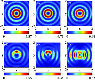
Figure 1: Distributions of $I^{z}_{1,k_{z}2}$ at a cross section for (a) $\Theta=0$, (b) $\Theta=\frac{\pi}{10}$, (c) $\Theta=\frac{\pi}{5}$, (d) $\Theta=\frac{3\pi}{10}$, (e) $\Theta=\frac{2\pi}{5}$, (f) $\Theta=\frac{\pi}{2}$. The units of $x$ and $y$ are in wavelengths.

In Fig. 1 are displayed the distributions of $I^{z}_{1,k_{z}2}$ at a cross section for different values of $\Theta$, where the units of $x$ and $y$ are in wavelengths. In order to illustrate the relative strength of longitudinal component, $I^{z}_{1,k_{z}2}$ is normalized in each part by the maximum of the corresponding beam’s intensity, $\max\{|\mathbf{E}_{1,k_{z}2}|^{2}\}$. It is seen that with the increase of $\Theta$, the longitudinal component of $\mathbf{E}_{1,k_{z}2}$ goes weaker. Only when the $\mathbf{I}$ is parallel to the $z$ axis, is the intensity of longitudinal component axially symmetric.

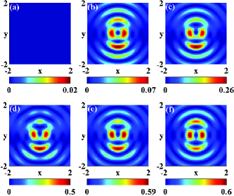
Figure 2: Distributions of $I^{z}_{2,k_{z}2}$ at a cross section for the same values of $\Theta$ as in Fig. 1. The units of $x$ and $y$ are in wavelengths.

For comparison, in Fig. 2 are displayed the distributions of $I^{z}_{2,k_{z}2}$ at a cross section for the same values of $\Theta$ as in Fig. 1, where the units of $x$ and $y$ are in wavelengths, and the $I^{z}_{2,k_{z}2}$ in each part is normalized as well by the maximum of the corresponding beam’s intensity, $\max\{|\mathbf{E}_{2,k_{z}2}|^{2}\}$. It is shown that with the increase of $\Theta$, the longitudinal component of $\mathbf{E}_{2,k_{z}2}$ goes stronger. When the $\mathbf{I}$ is parallel to the $z$ axis, the longitudinal component totally vanishes, in agreement with the fact that the $\mathbf{I}$ is perpendicular to $\mathbf{E}_{2,k_{z}l}$.

It seems to be an accepted criterion Martinez that whether a light beam can be viewed as a paraxial beam depends on whether its longitudinal component can be neglected in comparison with its transverse component. This should be valid when the characteristic vector $\mathbf{I}$ is perpendicular to the propagation direction, because all the diffraction-free beams in this case have negligible longitudinal components when the wavevector cone is close to the $z$ axis, as is shown in Eqs. (12). But we have noticed that when the $\mathbf{I}$ is parallel to the propagation direction, the beam associated with $\mathbf{E}_{2,k_{z}l}$ does not have longitudinal component, regardless of the cone angle of wavevector cone. Because large cone angles correspond to non-paraxial diffraction-free beams, the aforementioned criterion for a beam to be paraxial is not strictly valid. Such a criterion needs further exploration.

This work was supported in part by the National Natural Science Foundation of China (60877055 and 60806041) and the Shanghai Leading Academic Discipline Project (S30105).

References

(1) J. Durnin, J. Opt. Soc. Am. A 4, 651 (1987).
(2) J. Durnin, J. J. Miceli, Jr., and J. H. Eberly, Phys. Rev. Lett.
58, 1499 (1987).
(3) L. W. Davis and G. Patsakos, Opt. Lett. 6, 22 (1981).
(4) L. W. Davis and G. Patsakos, Phys. Rev. A 26, 3702 (1982).
(5) R. H. Jordan and D. G. Hall, Opt. Lett. 19, 427 (1994).
(6) D. G. Hall, Opt. Lett. 21, 9 (1996).
(7) K. S. Youngworth and T. G. Brown, Opt. Express. 7, 77
(2000).
(8) Z. Bouchal and M. Olivík, J. Mod. Opt. 42, 1555 (1995).
(9) M. Lax, W. H. Lousisell, and W. B. McKnight, Phy. Rev. A 11,
1365 (1975).
(10) C.-F. Li, Phys. Rev. A 78, 063831 (2008).
(11) A. I. Akhiezer and V. B. Berestetskii, Quantum electrodynamics
(Interscience Publishers, New York, 1965).
(12) S. J. Van Enk and G. Nienhuis, J. Mod. Opt. 41, 963 (1994).
(13) R. Martínez-Herrero, P. M. Mejías, and G. Piquero,
Characterization of Partially Polarized Light Fields (Springer-Verlag, Berlin, 2009).