Base-Station Selections for QoS Provisioning
Over Distributed Multi-User MIMO Links
in Wireless Networks

Abstract

We propose the QoS-aware BS-selection and the corresponding resource-allocation schemes for downlink multi-user transmissions over the distributed multiple-input-multiple-output (MIMO) links, where multiple location-independent base-stations (BS), controlled by a central server, cooperatively transmit data to multiple mobile users. Our proposed schemes aim at minimizing the BS usages and reducing the interfering range of the distributed MIMO transmissions, while satisfying diverse statistical delay-QoS requirements for all users, which are characterized by the delay-bound violation probability and the effective capacity technique. Specifically, we propose two BS-usage minimization frameworks to develop the QoS-aware BS-selection schemes and the corresponding wireless resource-allocation algorithms across multiple mobile users. The first framework applies the joint block-diagonalization (BD) and probabilistic transmission (PT) to implement multiple access over multiple mobile users, while the second one employs time-division multiple access (TDMA) approach to control multiple users’ links. We then derive the optimal BS-selection schemes for these two frameworks, respectively. In addition, we further discuss the PT-only based BS-selection scheme. Also conducted is a set of simulation evaluations to comparatively study the average BS-usage and interfering range of our proposed schemes and to analyze the impact of QoS constraints on the BS selections for distributed MIMO transmissions.

I Introduction

To increase the coverage of broadband wireless networks, distributed multiple-input-multiple-output (MIMO) techniques, where multiple location-independent base stations (BS) cooperatively transmit data to mobile users, have attracted more and more research attentions [2, 4, 3]. In particular, the distributed MIMO techniques can effectively organize multiple location-independent BS’s to form the distributed MIMO links connecting with mobile users Like the conventional centralized MIMO system [5, 7, 6], the distributed MIMO system can significantly enhance the capability of the broadband wireless networks in terms of the quality-of-service (QoS) provisioning as compared to the single antenna system. However, the distributed nature for cooperative multi-BS transmissions also imposes many new challenges in wide-band wireless communications, which are not encountered in the centralized MIMO systems. First, the cooperative distributed transmissions cause the severe difficulty for synchronization among multiple location-independent BS transmitters. Second, as the number of cooperative BS’s increases, the computational complexity for MIMO signal processing and coding also grow rapidly. Third, because the coordinated BS’s are located at different geographical positions, the cooperative communications in fact enlarge the interfering areas for the used spectrum, thus drastically degrading the frequency-reuse efficiency in the spatial domain. Finally, many wide-band transmissions are sensitive to the delay, and thus we need to design QoS-aware distributed MIMO techniques, such that the scarce wireless resources can be more efficiently utilized.

Towards the above issues, many research works on distributed MIMO transmissions have been proposed recently. The feasibility of transmit beamforming with efficient synchronization techniques over distributed MIMO link has been demonstrated through experimental tests [3], suggesting that complicated MIMO signal processing techniques are promising to implement in realistic systems. For the centralized MIMO system, the antenna selection [6, 7] is an effective technique to reduce the complexity, which clearly can be also extended to distributed MIMO systems for the BS selection. It can be expected that the BS-selection techniques can significantly decrease the processing complexity, while still achieving high throughput gain over the single BS transmission. Also, it is desirable to minimize the number of selected BS’s through BS-selection techniques, which can effectively decrease the interfering range and thus improve the frequency-reuse efficiency of the entire wireless network. Most previous research works for BS/antennas selections mainly focused on the scenarios of selecting a subset of BS’s/antennas with the fixed cardinality [6, 7, 4]. However, it is evident that based on the wireless-channel status, BS-subset selections with dynamically adjusted cardinality can further decrease the BS usage. More importantly, how to efficiently support diverse delay-QoS requirements through BS-selection in distributed MIMO systems sill remains a widely cited open problem.

To overcome the aforementioned problems, we propose the QoS-aware BS-selection schemes for the distributed wireless MIMO links, which aim at minimizing the BS usages and reducing the interfering range, while satisfying diverse statistical delay-QoS constraints. In particular, we develop two BS-usage minimization frameworks for distributed multi-suer MIMO transmissions. The first framework uses the joint block-diagonalization (BD) and probabilistic transmission (PT) for multiple access of multi-user over distributed MIMO links, while the second framework employs time-division multiple access (TDMA) techniques. We derive the optimal QoS-aware BS-selection and the corresponding resource allocation schemes for these two frameworks, respectively. We also discuss the PT-only based BS-selection scheme. Simulations are conducted for comparative analyses among the above BS-selection schemes.

The rest of this paper is organized as follows. Section II describes the system model for distributed MIMO transmissions. Section III introduces the statistical QoS guarantees and the concept of effective capacity. Section IV develops the joint BD and PT (BD-PT) optimization frameworks for QoS-aware BS-selections over multi-user distributed MIMO links and derives the corresponding optimal solution. Section V derives TDMA-based QoS-aware BS-selection scheme. Section VI conducts simulations to perform comparative analyses for our proposed schemes. The paper concludes with Section VII.

Notations: The operator $|\cdot|$ used on a real or complex number generates the absolute value; the operator $|\cdot|$ used for a set represents the cardinality of this set. We use boldface to denote matrices and vectors. For an $X\times Y$ matrix $\mathbf{A}$, we denote by $\mathbf{A}(i,j)$ the element on the $i$th row and $j$th column; $\|\mathbf{A}\|_{F}$ denotes the Frobenius norm of $\mathbf{A}$, where $\|\mathbf{A}\|_{F}\triangleq\sqrt{\sum_{i=1}^{X}\sum_{j=1}^{Y}|\mathbf{A}(i,j)|^{2}}$. The operators $(\cdot)^{\tau}$ and $(\cdot)^{{\dagger}}$ generate the transpose and conjugate transpose, respectively. The operator $1_{(\cdot)}$ is the indication function. If the statement in the subscript is true, we have $1_{(\cdot)}=1$; otherwise, $1_{(\cdot)}=0$.

II System Model

II-A System Architecture

We concentrate on the wireless distributed MIMO system for downlink transmissions depicted in Fig. 1, which consists of $K_{\mathrm{bs}}$ distributed BS’s, $K_{\mathrm{mu}}$ mobile users, and one central server. The $m$th BS has $M_{m}$ transmit antennas for $m=1,2,\ldots,K_{\mathrm{bs}}$ and the $n$th mobile user has $N_{n}$ receive antennas for $n=1,2,\ldots,K_{\mathrm{mu}}$. All distributed BS’s are connected to the central server through high-speed optical connections. The data to be delivered to the $n$th mobile user, $n=1,2,\ldots,K_{\mathrm{mu}}$, arrives at the central server with a constant rate, which is denoted by $\overline{C}_{n}$. Then, the central server dynamically controls these distributed BS’s to cooperatively transmit data to the corresponding mobile users under the specified delay-QoS requirements.

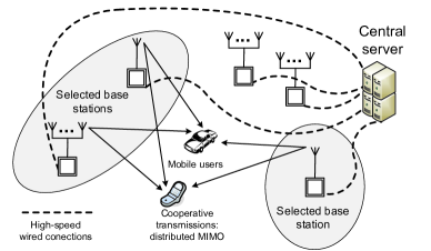
Figure 1: System model for wireless downlink distributed MIMO transmissions.

For multi-user downlink transmissions, the distributed BS’s and the mobile users form the broadcast MIMO link for data transmissions. The wireless fading channels between the $m$th BS and the $n$th mobile user is modeled by an $N_{n}\times M_{m}$ matrix $\mathbf{H}_{n,m}$, where $\mathbf{H}_{n,m}(i,j)$ is the complex channel gain between the $i$th receive antenna of $n$th mobile user and the $j$th transmit antenna of the $m$th BS. All elements of $\mathbf{H}_{n,m}$ are independent and circularly symmetric complex Gaussian random variables with zero mean and the variance equal to $\overline{h}_{n,m}$, implying that $\mathbf{H}$ has continuous cumulative distribution function (CDF). Also, the instantaneous aggregate power gain of the MIMO link between the $n$th mobile user and the $m$th BS, denoted by $\gamma_{n,m}$, is defined by

$$\gamma_{n,m}\triangleq\frac{1}{M_{m}}\left\|\mathbf{H}_{n,m}\right\|_{F}^{2}$$ (1)

Since the Frobenius norm of the channel matrix can effectively characterize the channel quality in terms of achieving high throughput [6], the aggregate power gain given in Eq. (1) will play an important role in our BS selection design. We further define $\mathbf{H}_{n}\triangleq[\mathbf{H}_{n,1}~{}\mathbf{H}_{n,2}~{}\cdots~{}\mathbf{H}_{n,K_{\mathrm{bs}}}]$ as the CSI for the $n$th mobile user for $n=1,2,\ldots,K_{\mathrm{mu}}$. The matrix $\mathbf{H}_{n}$ follows the independent block-fading model, where $\mathbf{H}_{n}$ does not change within a time period with the fixed length $T$, called a time frame, but varies independently from one frame to the other frame. Furthermore, we define $\mathbf{H}\triangleq[\mathbf{H}_{1}^{\tau}~{}\mathbf{H}_{2}^{\tau}~{}\cdots~{}\mathbf{H}_{K_{\mathrm{bs}}}^{\tau}]^{\tau}$, representing a fading state of the entire distributed MIMO system.

In order to decrease the complexity and suppress the interfering range of the distributed MIMO transmission, the cental server dynamically selects a subset of BS’s to construct the distributed MIMO link. Then, our design target is to minimize the average number of needed BS’s subject to the specified QoS constraints. We suppose that each mobile user can perfectly estimate its CSI at the beginning of every time frame and reliably feed CSI back to the central server through dedicated control channels. Based on CSI $\mathbf{H}$ and QoS requirements, the central server then adaptively selects the subset of BS’s and organizes them to transmit data to mobile users through the distributed MIMO links.

II-B The Delay QoS Requirements

The central data server maintains a queue for the incoming traffic to each mobile user. We mainly focus on the queueing delay in this paper because the wireless channel is the major bottleneck for high-rate wireless transmissions. Since it is usually unrealistic to guarantee the hard delay bound over the highly time-varying wireless channels, we employ the statistical metric, namely, the delay-bound violation probability, to characterize the diverse delay QoS requirements. Specifically, for the $n$th mobile user, the probability of violating a specified delay bound, denoted by $D_{\mathrm{th}}^{(n)}$, cannot exceed a given threshold $\xi_{n}$. That is, the inequality

$$\mbox{Pr}\left\{D_{n}>D_{\mathrm{th}}^{(n)}\right\}\leq\xi_{n},\quad n=1,2,\ldots,N_{\mathrm{mu}},$$ (2)

needs to hold, where $D_{n}$ denotes the queueing delay in the $n$th mobile user’s queueing system.

II-C Performance Metrics and Design Objective

We denote by $L$ the cardinality of the selected BS subset (the number of selected BS’s) for the distributed MIMO transmission in a fading state. Then, we denote the expectation of $L$ by $\overline{L}$ and call it the average BS usage. As mentioned in Section II-A, our major objective is to minimize $\overline{L}$ through dynamic BS selection while guaranteeing the delay QoS constraint specified by Eq. (2). We will also evaluate the average interfering range affected by the distributed MIMO transmission. The instantaneous interfering range, denoted by $A$, is defined as the area of the region where the average received power under the current MIMO transmission is larger than then certain threshold denoted by $\sigma^{2}_{\mathrm{th}}$. The average interfering area is then defined as the expectation $\mathbb{E}_{\mathbf{H}}\{A\}$ over all $\mathbf{H}$. Clearly, minimizing $\overline{L}$ can not only reduce implementation complexity, but also decrease the average interfering range affected by the transmit power.

II-D The Power Control Strategy

The transmit power of our distributed MIMO system varies with the number of selected BS’s. In particular, given the number $L$ of selected BS’s, the total instantaneous transmitted power used for distributed MIMO transmissions is set as a constant equal to $\mathcal{P}_{L}$. Furthermore, $\mathcal{P}_{L}$ linearly increases with $L$ by using the strategy as follows:

$$\mathcal{P}_{L}=\mathcal{P}_{\mathrm{ref}}+\kappa(L-1),\quad L=1,2,\ldots,K_{\mathrm{bs}},$$ (3)

where $\mathcal{P}_{\mathrm{ref}}>0$ is called the reference power and $\kappa\geq 0$ describes the power increasing rate against $L$. Also, we define $\mathcal{P}_{L}\triangleq 0$ for $L=0$. The above power adaptation strategy is simple to implement, while the average transmit power can be effectively decreased through minimizing the average number of used BS’s. In addition, Eq. (3) can upper-bound the instantaneous interferences and the interfering range over the entire network.

III Effective Capacity Approach for Statistical Delay-QoS Guarantees

In this paper, we apply the effective capacity approach [9, 12, 10, 18] to integrate the constraint on delay-bound violation probability given by Eq. (2) into our BS selection design. Consider a stable discrete-time queueing system with the stationary time-varying arrival-rate and departure-rate (service-rate) processes. The asymptotic analyses based on the large deviation principal [9, 8] show that under the sufficient conditions, the probability that the queue-length, denoted by $Q$, exceeding a given bound $Q_{\mathrm{th}}$ can be approximated by

$$\mbox{Pr}\{Q>Q_{\mathrm{th}}\}\approx e^{-\theta Q_{\mathrm{th}}},$$ (4)

where $\theta>0$ is a constant called QoS exponent. It is clear that the larger (smaller) $\theta$ implies the lower (higher) queue-length-bound violation probability.

By using $\theta$, the delay-bound violation probability can be approximated [9] by

$$\mbox{Pr}\{D>D_{\mathrm{th}}\}\approx e^{-\theta\overline{C}D_{\mathrm{th}}}.$$ (5)

for the constant rate $\overline{C}$. When the arrival rate is not time-varying, the approximation in Eq. (5) needs to replace $\overline{C}$ with effective bandwidth [9, 8] function of the arrival rate process, which is defined as the minimum constant service rate required to guarantee QoS exponent $\theta$.

Then, to upper-bound $\mbox{Pr}\{D>D_{\mathrm{th}}\}$ with a threshold $\xi$, using Eq. (5), we get the minimum required QoS exponent $\theta$ as follows:

$$\theta=-\frac{\log(\xi)}{\overline{C}D_{\mathrm{th}}}.$$ (6)

Consider a discrete-time arrival process with constant rate $\overline{C}$ and a discrete-time time-varying stationary departure process, denoted by $R[k]$, where $k$ is the time index. In order to guarantee the desired $\theta$ determined by Eq. (6), the statistical QoS theory [8, 9] shows that the effective capacity $\mathcal{C}(\theta)$ of the service-rate process $R[k]$ needs to satisfy

$$\mathcal{C}(\theta)=\overline{C},$$ (7)

given the QoS exponent $\theta$. The effective capacity function is defined in [9] as the maximum constant arrival rate which can be supported by the service rate to guarantee the specified QoS exponent $\theta$. If the service-rate sequence $R[k]$ is time uncorrelated, the effective capacity can be written [12] as

$$\mathcal{C}(\theta)\triangleq-\frac{1}{\theta}\log\left(\mathbb{E}\left\{e^{-\theta R[k]}\right\}\right),$$ (8)

where $\mathbb{E}\{\cdot\}$ denotes the expectation.

In our distributed MIMO system, the BS selection result is designed as the function determined by the current CSI. Thus, the corresponding transmission rate (service rate) is time independent under the independent block-fading model (see Section II-A). Then, applying Eqs. (6)-(7), the delay QoS constraints given by Eq. (2) can be equivalently converted to:

$$\mathbb{E}_{\mathbf{H}}\left\{e^{-\theta_{n}R_{n}}-e^{-\theta_{n}\overline{C}_{n}}\right\}\leq 0,\quad,n=1,2,\ldots,N_{\mathrm{mu}},$$ (9)

where $\theta_{n}=-\log(\xi_{n})\!\!\left/\!\big{(}\overline{C}_{n}D_{\mathrm{th}}^{(n)}\big{)}\right.$ and $\mathbb{E}_{\mathbf{H}}\{\cdot\}$ denotes the expectation over all $\mathbf{H}$.

IV Joint Block-Diagonalization and Probabilistic Transmission Based Base-Station Selection

As discussed in Section II, based on CSI $\mathbf{H}$ and QoS requirements, the central server will adaptively select the subset of BS’s and organizes them to transmit data to mobile users through the distributed MIMO links. Given the cardinality $L$ of the desired BS subset in a fading state, we denote by $\Omega_{L}$ the set of indices of selected BS’s, where $\Omega_{L}=\{i_{L,1},i_{L,2},\ldots,i_{L,L}\}$ and $i_{L,\ell}\in\{1,2,\ldots,K_{\mathrm{bs}}\}$ for $\ell=1,2,\ldots,L$. Note that once a BS is selected, we use all its transmit antennas for data transmissions. For the specified $L$, we use $\mathcal{U}_{L}=\{n_{U,1},n_{U,2},\ldots,n_{U,U}\}$ to denote the set of active users, picked by the central server, which can receive the data in this fading state, where $U$ is the cardinality of $\mathcal{U}_{L}$. For presentation convenience, we use $\mathfrak{M}_{L}\triangleq(\Omega_{L},\mathcal{U}_{L})$ to represent a specific transmission mode (or mode in short). Moreover, we term the pairs with $U\geq 2$ for $\mathcal{U}_{L}$ as multi-user modes, and term the pairs with $U=1$ as single-user modes.

Given $L$, $\Omega_{L}$ and $\mathcal{U}_{L}$, the channel matrix of the $n$th mobile user for $n\in\mathcal{U}_{L}$, modeled by $\mathbf{H}_{\Omega_{L}}^{(n)}$, is determined by

$$\mathbf{H}_{\Omega_{L}}^{(n)}\triangleq\left[\mathbf{H}_{n,i_{L,1}}~{}\mathbf{H}_{n,i_{L,2}}~{}\cdots~{}\mathbf{H}_{n,i_{L,L}}\right],$$ (10)

where $\mathbf{H}_{\Omega_{L}}^{(n)}$ is an $N_{n}\times\big{(}\sum_{\ell\in\Omega_{L}}M_{i_{L,\ell}}\big{)}$ matrix. Furthermore, we use $\overline{\boldsymbol{\Upsilon}}_{\Omega_{L}}^{(n)}$ to denote the power gain matrix for $\mathbf{H}_{\Omega_{L}}^{(n)}$ under the given $\Omega_{L}$, where

$$\overline{\boldsymbol{\Upsilon}}_{\Omega_{L}}^{(n)}(i,j)=\mathbb{E}_{\mathbf{H}}\left\{\left.\left|\mathbf{H}_{\Omega_{L}}^{(n)}(i,j)\right|^{2}\right|\mbox{fixing}~{}\Omega_{L}\right\}.$$ (11)

The physical-layer signal transmissions can be modeled by

$$\begin{array}[]{l}\mathbf{y}_{\mathfrak{M}_{L}}^{(n)}=\mathbf{H}_{\Omega_{L}}^{(n)}\sum_{i\in\mathcal{U}_{L}}\mathbf{s}_{\mathfrak{M}_{L}}^{(i)}+\boldsymbol{\varsigma}^{(n)},\quad n\in\mathcal{U}_{L},\end{array}$$ (13)

where $\mathbf{s}_{\mathfrak{M}_{L}}^{(i)}$ represents the $i$th user’s input signal vector for the MIMO channel $\mathbf{H}_{\Omega_{L}}^{(i)}$, $\mathbf{y}_{\mathfrak{M}_{L}}^{(n)}$ is the signal vector received by the $n$th user, and $\boldsymbol{\varsigma}^{(n)}$ is the complex additive white Gaussian noise (AWGN) vector with unit power for each element of this vector. In this section, we employ the block-diagonalization (BD) technique [15] to implement multiple access for multi-user modes in our QoS-aware BS-selection framework.

For dynamic BS selections in distributed MIMO transmissions, $L$ and $\mathfrak{M}_{L}$ are both functions of CSI and QoS requirements. Then, we need to answer the following questions: (i) Given $L$, which transmission mode will be used for single-user and multi-user modes, respectively? (ii) When do we use single-user or multi-user modes? (iii) For a specific multi-user mode, how do we quantitatively allocate the wireless resources across multiple mobile users under the BD based transmissions? (iv) Which $L$ will be selected for distributed MIMO transmissions in each fading state to decrease the average BS-usage while satisfying the QoS requirements?

Clearly, we can not examine all combinations of $(\Omega_{L},\mathcal{U}_{L})$ to minimize the BS usage due to the too high complexity. Then, in Section IV-A, we develop the heuristic algorithms to efficiently select $\mathfrak{M}_{L}$ for the specified $L$ in multi-user transmission modes. In Section IV-B, we determine how to select $\mathfrak{M}_{L}$ in single-user transmission mode. Based on schemes developed in Sections IV-A and IV-B, we further answer questions (iii) and (iv) through formulating and solving the joint BD-PT based BS-usage minimization problem in Sections IV-C and IV-D.

IV-A Selection of $\mathfrak{M}_{L}$ in Multi-User Transmission Modes

In each fading state, we pick $K_{\mathrm{bs}}$ multi-user transmission modes as candidates for distributed MIMO transmissions. These $K_{\mathrm{bs}}$ transmission modes corresponds to $L=1,2,\ldots,K_{\mathrm{bs}}$, respectively, representing different levels of BS usages. As mentioned previously, the derivation of global optimal selection strategy in terms of minimizing the average BS usage is intractable, since the complexity of examining all possible $\mathfrak{M}_{L}=(\Omega_{L},\mathcal{U}_{L})$ is too high. Therefore, for a given $L$, we determine $\mathfrak{M}_{L}$ through a two-step method. We first propose the priority BS-selection to determine the BS subset $\Omega_{L}$. Then, based on the selected $\Omega_{l}$, we derive $\mathcal{U}_{L}$ through a joint channel-priority user-selection process.

A.1. Priority BS-Selection to Determine $\Omega_{L}$

Consider any fading state $\mathbf{H}$. The $n$th user’s global maximum achievable transmission rate is attained when all BS’s are used and all the other users do not transmit. In this case, we have $L=K_{\mathrm{bs}}$ and $\mathbf{H}_{\Omega_{L}}^{(n)}\!\!\!=\mathbf{H}_{n}$. Moreover, all BS’s and the $n$th user builds a single-user MIMO channel $\mathbf{H}_{n}$. Then, the maximum achievable rate is equal to the capacity for the MIMO channel $\mathbf{H}_{n}$ with power $\mathcal{P}_{L}$, which is given by [5]

$$R^{(n)}_{\max} \!\!\!\!\!= \!\!\!\!\max_{\boldsymbol{\Xi}^{(n)}:\mathrm{Tr}\left(\boldsymbol{\Xi}^{(n)}\right)=\mathcal{P}_{K_{\mathrm{bs}}}}\!\!\!\left\{\!BT\!\log\left[\det\left(\mathbf{I}+\mathbf{H}_{n}\boldsymbol{\Xi}^{(n)}\mathbf{H}_{n}^{{\dagger}}\right)\right]\right\}$$

where $\det(\cdot)$ generates the determinant of a matrix, $\mathrm{Tr}(\cdot)$ evaluates the trace of a matrix, and $\boldsymbol{\Xi}^{(n)}$ is the covariance matrix of $\mathbf{s}_{\mathfrak{M}_{L}}^{(n)}$. Correspondingly, we get the maximum achievable effective capacity of the $n$th user, denoted by $\mathcal{C}_{\max}^{(n)}$, as follows:

$$\mathcal{C}_{\max}^{(n)}=-\frac{1}{\theta_{n}}\log\left(\mathbb{E}_{\mathbf{H}}\left\{e^{-\theta_{n}R^{(n)}_{\max}}\right\}\right),$$ (14)

for $n=1,2,\ldots,K_{\mathrm{mu}}$. Furthermore, we define the effective-capacity fraction for the $n$th user as the ratio between the traffic loads and the maximum achievable effective capacity. Denoting the effective-capacity fraction by $\widehat{C}_{n}$, we define $\widehat{C}_{n}\triangleq\overline{C}_{n}/\mathcal{C}_{\max}^{(n)}$. Note that $\widehat{C}_{n}$ can be readily obtained off-line based on the statistical information of wireless channels, and thus can be used to design the BS selection algorithm during the data transmission process. For presentation convenience, we sort $\{\widehat{C}_{n}\}_{n=1}^{K_{\mathrm{mu}}}$ in the decreasing order and denote the permuted version by $\{\widehat{C}_{\pi(j)}\}_{h=1}^{K_{\mathrm{mu}}}$, where $\widehat{C}_{\pi(1)}\geq\widehat{C}_{\pi(2)}\geq\cdots\geq\widehat{C}_{\pi(K_{\mathrm{mu}})}$ indicates the order from the higher priority to the lower priority. In the rest of this paper, we use the term of user $\pi(i)$ to denote the user associated with the $i$th largest effective-capacity fraction.

Clearly, for a higher $\widehat{C}_{n}$, the $n$th user needs more wireless resources to meet its QoS requirements. Thus, in order to satisfy the QoS requirements for all users, we assign higher BS-selection priority to the user with larger $\widehat{C}_{n}$. Following this principle, we design the priority BS-selection algorithm to determine $\Omega_{L}$ in each fading state and provide the pseudo code in Fig. 2. In the pseudo code given by Fig. 2, we use temporary variables $\overline{\Psi}$ and $\Psi$ to denote the subsets of BS’s which have been selected and which have not been selected, respectively.

01. Let $\Psi:=\{1,2,\ldots,K_{\mathrm{bs}}\}$, $\overline{\Psi}:=\varnothing$, and $\ell=|\overline{\Psi}|$; ! Initialization 02. $j:=1$.      ! Start selection with User $\pi(1)$ 03. WHILE $(\ell<L)$  ! Iterative selections until $L$ BS’s are selected 04.   $m^{*}=\arg\min_{m\in\Psi}\{\gamma_{\pi(j),m}\}$.     ! User $\pi(j)$ selects the BS with the largest aggregate power gain. 05.   $\overline{\Psi}:=\overline{\Psi}\cup\{m^{*}\}$, $\Psi:=\Psi-\{m^{*}\}$, and $\ell:=\ell+1$.     ! Update $\overline{\Psi}$, $\Psi$, and $\ell$. 06.   IF $j=K_{\mathrm{mu}}$, then $j:=1$; ELSE $j:=j+1$.     ! Let next user with lower priority to select BS. 07. END 08. $\Omega_{L}:=\overline{\Psi}$.    ! Complete the BS selection and get $\Omega_{L}$.

Figure 2: The pseudo codes to determine $\Omega_{L}$ in each fading state by using the priority BS-selection algorithm for the multi-user transmissions.

As shown in Fig. 2, in each fading state the BS-selection procedure starts with the selection for user $\pi(1)$, who has the highest priority. After picking one BS for user $\pi(1)$, we select one different BS for user $\pi(2)$. More generally, after selecting for user $\pi(j)$, we choose one BS for user $\pi(j+1)$ from the BS-subset $\Psi$, which consists of the BS’s that have not been selected. This procedure repeats until $L$ BS’s are selected. For user-$\pi(j)$’s selection, we choose the BS with the maximum aggregate power gain over the subset $\Psi$, where $\gamma_{\pi(j),m}$ denotes the instantaneous aggregate power gain between user $\pi(j)$ and the $m$th BS (see Eq. (1) for its definition). In addition, after user-$\pi(K_{\mathrm{mu}})$’s selection, if the number of selected BS’s is still smaller than $L$, we continue selecting one more BS for user $\pi(1)$, as shown in line 06 in Fig. 2, and repeat this iterative selection procedure until having selected $L$ BS’s. Clearly, users with higher priorities benefitted more from the above algorithm. Also note that the mobile users’ priority order is determined by the effective-capacity fraction, which adapts to the mobile users’ QoS requirements.

A.2. The Principle of the Block Diagonalization Technique

The block-diagonalization (BD) precoding techniques [15] have been widely used for MIMO transmissions because of its low complexity. In this section, we also apply the BD technique for our QoS-aware BS selection framework. For completeness of this paper, the principles of the BD technique are summarized as follows.

Given transmission mode $\mathfrak{M}_{L}=(\Omega_{L},\mathcal{U}_{L})$, the idea of block diagonalization [15] is to use a precoding matrix, denoted by $\boldsymbol{\Gamma}_{\mathfrak{M}_{L}}^{(n)}$, for the $n$th user’s transmitted signal vector, where $n=n_{u}\in\mathcal{U}_{L}$ for some $u$, such that $\mathbf{H}_{\Omega_{L}}^{(i)}\boldsymbol{\Gamma}_{\mathfrak{M}_{L}}^{(n)}=\mathbf{0}$ for all $i$ satisfying $i\neq n$ and $i\in\mathcal{U}_{L}$. By setting $\mathbf{s}_{\mathfrak{M}_{L}}^{(n)}=\boldsymbol{\Gamma}_{\mathfrak{M}_{L}}^{(n)}\widehat{\mathbf{s}}_{\mathfrak{M}_{L}}^{(n)}$, where $\widehat{\mathbf{s}}_{\mathfrak{M}_{L}}^{(n)}$ is the $n$th user’s data vector to be precoded by $\boldsymbol{\Gamma}_{\mathfrak{M}_{L}}^{(n)}$, we can rewrite the received signal $\mathbf{y}_{\mathfrak{M}_{L}}^{(n)}$ as

$$\begin{array}[]{l}\mathbf{y}_{\mathfrak{M}_{L}}^{(n)}=\mathbf{H}_{\Omega_{L}}^{(n)}\sum_{i\in\mathcal{U}_{L}}\boldsymbol{\Gamma}_{\mathfrak{M}_{L}}^{(i)}\widehat{\mathbf{s}}_{\mathfrak{M}_{L}}^{(i)}+\boldsymbol{\varsigma}^{(n)}=\widehat{\boldsymbol{\Gamma}}_{\mathfrak{M}_{L}}^{(n)}\widehat{\mathbf{s}}_{\mathfrak{M}_{L}}^{(n)}+\boldsymbol{\varsigma}^{(n)},\end{array}$$ (16)

where $\widehat{\boldsymbol{\Gamma}}_{\mathfrak{M}_{L}}^{(n)}\triangleq\mathbf{H}_{\Omega_{L}}^{(n)}\boldsymbol{\Gamma}^{(n)}_{\mathfrak{M}_{L}}$. Under this strategy, the $n$th user’s signal will not cause interferences to other active users. Accordingly, the MIMO broadcast transmissions are virtually converted to $U$ orthogonal MIMO channels with channel matrices $\big{\{}\widehat{\boldsymbol{\Gamma}}_{\mathfrak{M}_{L}}^{(n)}\big{\}}_{n\in\mathcal{U}_{L}}$. Thus, the $n$th user’s maximum achievable rate, denoted by $R^{(n)}_{\mathfrak{M}_{L}}\big{(}\mathcal{P}_{L}^{(n)}\big{)}$, is equal to the capacity of the equivalent MIMO channel $\widehat{\boldsymbol{\Gamma}}_{\mathfrak{M}_{L}}^{(n)}$, as follows:

$$~{}R^{(n)}_{\mathfrak{M}_{L}}\!\big{(}\mathcal{P}_{L}^{(n)}\big{)}\!\triangleq\max_{\boldsymbol{\Xi}^{(n)}}\!\left\{\!BT\log\!\left[\det\!\!\left(\!\mathbf{I}+\widehat{\boldsymbol{\Gamma}}_{\mathfrak{M}_{L}}^{(n)}\boldsymbol{\Xi}^{(n)}\!\!\left(\widehat{\boldsymbol{\Gamma}}_{\mathfrak{M}_{L}}^{(n)}\right)^{\!\!{\dagger}}\right)\!\right]\!\right\}$$

subject to $\mathrm{Tr}\big{(}\boldsymbol{\Xi}^{(n)}\big{)}=\mathcal{P}_{L}^{(n)}$ for $n\in\mathcal{U}_{L}$, where $\boldsymbol{\Xi}^{(n)}$ is the covariance matrix of $\widehat{\mathbf{s}}_{\mathfrak{M}_{L}}^{(n)}$ and $\mathcal{P}_{L}^{(n)}$ denotes the power allocated for the $n$th user under mode $\mathfrak{M}_{L}$. Correspondingly, we will set the service rate $R_{n}$ of the $n$th user equal to $R^{(n)}_{\mathfrak{M}_{L}}\big{(}\mathcal{P}_{L}^{(n)}\big{)}$. Note that $\boldsymbol{\Gamma}_{\mathfrak{M}_{L}}^{(n)}$ may not exist, which then results in a service rate equal to 0. Also, we set $R_{n}=R^{(n)}_{\mathfrak{M}_{L}}\big{(}\mathcal{P}_{L}^{(n)}\big{)}=0$ for $n\notin\mathcal{U}_{L}$ or $L=0$. For the procedures to determine the precoding matrix $\boldsymbol{\Gamma}_{\mathfrak{M}_{L}}^{(n)}$ of the $n$th user, where $n=n_{u}\in\mathcal{U}_{L}$ for some $u$, please refer to [15].

A.3. Derivation of Active-User Set $\mathcal{U}_{L}$

Note that given $\Omega_{L}$ we may not be able to accommodate all users, because of the limited number transmit antennas. Although several algorithms for selecting active-user set have been proposed [16, 17], they cannot be applied in the framework of this paper, because the QoS provisioning for mobile users are not addressed those in these algorithms. Next, we determine $\mathcal{U}_{L}$ through a joint channel-priority method for active user selections. The pseudo code of this algorithm is provided in Fig. 3.

01. Let $\Lambda:=\{1,2,\ldots,K_{\mathrm{mu}}\}$, $\overline{\Lambda}:=\varnothing$, and $M_{\Sigma}\triangleq\sum_{\ell\in\Omega}M_{\ell}$. 02. WHILE $(\Lambda\neq\varnothing)$ 03.   For all $n\in\Lambda$ 04.     Temporarily setting $\mathcal{U}_{L}:=\overline{\Lambda}\cup\{n\}$. 05.     Get $\boldsymbol{\Gamma}_{\mathfrak{M}_{L}}^{(n)}$. Then, set $\displaystyle~{}~{}~{}~{}\varpi_{n}$ $\displaystyle\!\!\!\!\!\!\!:=$ $\displaystyle\!\!\!\!\!\!\frac{1}{M_{\Sigma}}\mathbb{E}_{\mathbf{H}}\left\{\left\|\mathbf{H}_{\Omega_{L}}^{(n)}\boldsymbol{\Gamma}_{\mathfrak{M}_{L}}^{(n)}\right\|_{F}^{2}\left|\mbox{Fixing}~{}\boldsymbol{\Gamma}_{\mathfrak{M}_{L}}^{(n)}\right.\right\}$ $\displaystyle\!\!\!\!\!\!\!=$ $\displaystyle\!\!\!\!\!\!\frac{1}{M_{\Sigma}}\overline{\boldsymbol{\Upsilon}}_{\Omega_{L}}^{(n)}\left[\mathrm{conj}\left(\boldsymbol{\Gamma}_{\mathfrak{M}_{L}}^{(n)}\right)\circ\boldsymbol{\Gamma}_{\mathfrak{M}_{L}}^{(n)}\right],$     where $\overline{\boldsymbol{\Upsilon}}_{\Omega_{L}}^{(n)}$ is given by Eq. (11); $(\cdot\circ\cdot)$ generates     element-wise product between two matrices with the same size;     $\mathrm{conj}(\cdot)$ yields the element-wise conjugation. 06.     Set $\displaystyle~{}~{}~{}~{}\widehat{\gamma}_{n}\!:=\!\left\{\!\begin{array}[]{ll}1,&\mbox{if}~{}0<\varpi_{n}\leq\frac{1}{M_{\Sigma}}\left\|\mathbf{H}_{\Omega_{L}}^{(n)}\boldsymbol{\Gamma}_{\mathfrak{M}_{L}}^{(n)}\right\|_{F}^{2};\\ 0,&\mbox{otherwise}.\end{array}\right.$ (20) 07.   END 08.   Select $\widehat{u}$ such that for all $j\in\Lambda$, $j\neq\widehat{u}$, the following condition $\displaystyle~{}~{}~{}(\widehat{\gamma}_{\widehat{u}}>\widehat{\gamma}_{j})~{}\mbox{or}~{}(\widehat{\gamma}_{\widehat{u}}=\widehat{\gamma}_{j}~{}\&~{}\mbox{user}~{}\widehat{u}~{}\mbox{has higher priority than user $j$})$   holds, where the priority order is determined in Section IV-A.1. 09.   IF $\varpi_{\widehat{u}}>0$, $\overline{\Lambda}:=\overline{\Lambda}\cup\{\widehat{u}\}$ and $\Lambda:=\Lambda-\{\widehat{u}\}$; else BREAK. 10. END 11. Set $\mathcal{U}_{L}:=\overline{\Lambda}$.

Figure 3: Pseudo codes of the block-diagonalization based joint channel-priority algorithm to determine the active-user set $\mathcal{U}_{L}$ in each fading state.

In the joint channel-priority algorithm provided by Fig. 3, we iteratively select users one by one into the set $\mathcal{U}_{L}$. In particular, we use variables $\Lambda$ and $\overline{\Lambda}$ to represent the temporary sets of users which have and have not been selected, respectively. As shown in Fig. 3, lines 02 through 10 describe loops for iterative user selection, where we pick one user in each loop until all users are selected (i.e., $\Lambda=\varnothing$) or no more user can be accommodated (examined by line 12). Within each loop, given the existing active-user set $\overline{\Lambda}$ we examine the channel quality of each user after BD. Specifically, we first get the BD precoding matrix of the $n$th user. Then, we derive $\varpi_{n}$, which is average channel-power-gain after BD over all transmit antennas, representing the average channel quality, and also obtain $\|\mathbf{H}_{\Omega_{L}}^{(n)}\boldsymbol{\Gamma}_{\mathfrak{M}_{L}}^{(n)}\|_{F}^{2}/M_{\Sigma}$ line 06, which characterizes the instantaneous channel quality. We further define a variable $\widehat{\gamma}_{n}$, as shown in line 07, where $\widehat{\gamma}_{n}=1$ and $\widehat{\gamma}_{n}=0$ indicate that the channel quality is above and below the average level, respectively. Obtaining $\widehat{\gamma}_{n}$, our selection criteria are as follows. First, we desire to select the user with higher $\widehat{\gamma}_{n}$, implying that this user’s current channel is better compared with its statistical channel qualities, which will more efficiently use the system resources towards this user’s QoS requirement. Second, if two users have the same $\widehat{\gamma}_{n}$, we will select the user with higher priority. Following this criterion, in line 08, we pick the unique user from $\Lambda$ in the current loop, whose index is denoted $\widehat{u}$. However, if $\varpi_{\widehat{u}}=0$, implying the maximum achievable rate equal 0. As a result, no more user can be admitted, including the $\widehat{u}$th user. We will then terminate the loop, as shown in line 09, to finish the selection process.

IV-B BS Selection in Single-User Transmission Modes

For single-user transmission modes, we have $\mathcal{U}_{L}=\{n\}$, $n\in\{1,2,\ldots,K_{\mathrm{mu}}\}$. Thus, at any time instant, there is only one user receiving data from multiple BS’s through a single-user MIMO channel $H_{\Omega_{L}}^{(n)}$. Accordingly, the maximum achievable rate for the $n$th user is equal to the capacity of $H_{\Omega_{L}}^{(n)}$ with power $\mathcal{P}_{L}$, which is denoted by $R_{\Omega_{L}}^{(n)}$. However, even for the single-user case, the complexity of high of choosing $\Omega_{L}$ to maximize the achievable data rate is too high, since we need to examine all $K_{\mathrm{bs}}\choose L$ combinations. Norm-based antenna selections have been demonstrated to be effective in achieving high system throughput with low complexity in centralized MIMO system [6, 7], which can be also extended to BS-selection in distributed MIMO system. Specifically, for the $n$th user with specified $L$ in our framework, we select BS’s with $L$ largest aggregate channel power gain. As a result, in each fading state we have $K_{\mathrm{bs}}K_{\mathrm{mu}}$ single-user modes as candidates for distributed MIMO transmissions. Given the transmission mode with $\Omega_{L}$ and the active user $n$, we will set the service rate $R_{n}$ equal to $R_{\Omega_{L}}^{(n)}$.

IV-C The Optimization Framework for Transmission Mode Selection and Resource Allocation

We have derived candidate $(\Omega_{L},\mathcal{U}_{L})$ in multi-user and single-user transmissions modes, respectively. We still need to answer how to allocate power over different mobile users in multi-user modes and which transmission mode will be eventually used for distributed MIMO transmissions. In this section, we employ the probabilistic transmission to determine finally selecting which transmission mode. Specifically, we use multi-user mode $(\Omega_{L},\mathcal{U}_{L})$ determined through algorithms given in Figs. 2 and 3 with a probability denoted by $\phi_{L}$, $L=0,1,2,\ldots,K_{\mathrm{bs}}$; also, we use single-user mode with BS-subset cardinality $L$ and $\mathcal{U}_{L}$ with a probability denoted by $q_{L,n}$, $L=1,2,\ldots,K_{\mathrm{bs}}$, $n=1,2,\ldots,K_{\mathrm{mu}}$. Note that $\phi_{0}$ is the probability of the case that nothing is transmitted. Clearly, the sum over all $q_{L,n}$ and $\phi_{L}$ must be equal to 1. For multi-user mode, we denote power allocated to the $n$th user in transmission mode $(\Omega_{L},\mathcal{U}_{L})$ by $\mathcal{P}_{L}^{(n)}$, while the total power constraint is given by Eq. (3). For presentation convenience, we further define $\boldsymbol{\phi}\triangleq(\phi_{1},\phi_{2},\ldots,\phi_{K_{\mathrm{mu}}})$ and $\mathbf{q}\triangleq(\mathbf{q}_{1},\mathbf{q}_{2},\ldots,\mathbf{q}_{K_{\mathrm{bs}}})$ with $\mathbf{q}_{L}\triangleq(q_{L,1},q_{L,2},\ldots,q_{L,K_{\mathrm{mu}}})$ to describe the probabilistic transmission policy; we also define $\boldsymbol{\mathcal{P}}\triangleq\big{(}\boldsymbol{\mathcal{P}}_{1},\boldsymbol{\mathcal{P}}_{2},\ldots,\boldsymbol{\mathcal{P}}_{K_{\mathrm{bs}}}\big{)}$ with $\boldsymbol{\mathcal{P}}_{L}\triangleq\big{(}\mathcal{P}_{L}^{(1)},\mathcal{P}_{L}^{(2)},\ldots,\mathcal{P}_{L}^{(K_{\mathrm{mu}})}\big{)}$ to characterize the power allocation policy in multi-user modes. Then, we formulate the following optimization problem $\boldsymbol{A1}$ to derive the efficient transmission-mode selection and the corresponding power allocation policy:

$\boldsymbol{A1}$: Joint BD-PT based BS-usage minimization

$$\min_{(\boldsymbol{\phi},\mathbf{q},\boldsymbol{\mathcal{P}})}\left\{\mathbb{E}_{\mathbf{H}}\left\{\sum_{L=1}^{K_{\mathrm{bs}}}L\left(\phi_{L}+\sum_{n=1}^{K_{\mathrm{mu}}}q_{L,n}\right)\right\}\right\}$$

$$\mbox{s.t.: }\,1).~{}\sum_{L=0}^{K_{\mathrm{bs}}}\phi_{L}+\sum_{L=1}^{K_{\mathrm{bs}}}\sum_{n=1}^{K_{\mathrm{mu}}}q_{L,n}=1,\quad\quad\forall\,\mathbf{H}$$ (21)

$$2).~{}\sum_{n=1}^{K_{\mathrm{mu}}}\mathcal{P}_{L}^{(n)}=\mathcal{P}_{L},\quad\quad\forall\,L,\,\mathbf{H};$$ (22)

$$3).~{}\mathbb{E}_{\mathbf{H}}\!\left\{\sum_{L=0}^{K_{\mathrm{bs}}}\!\left(\!\phi_{L}e^{-\theta_{n}R^{(n)}_{\mathfrak{M}_{L}}\big{(}\mathcal{P}_{L}^{(n)}\big{)}}+q_{L,n}e^{-\theta_{n}R^{(n)}_{\Omega_{L}}}\!\right)\right.$$

$$\quad\quad\quad\quad\quad\quad+\sum_{L=0}^{K_{\mathrm{bs}}}\sum_{j,j\neq n}q_{L,j}\Bigg{\}}-e^{-\theta_{n}\overline{C}_{n}}\leq 0,~{}\forall\,n.\!\!\!\!\!\!\!\!\!\!\!\!$$ (23)

IV-D Derivations of the Optimal Solution of Problem $\boldsymbol{A1}$

D.1. The Properties of $R^{(n)}_{\mathfrak{M}_{L}}\big{(}\mathcal{P}_{L}^{(n)}\big{)}$

Before solving $\boldsymbol{A1}$, we first summarize the properties of $R^{(n)}_{\mathfrak{M}_{L}}\big{(}\mathcal{P}_{L}^{(n)}\big{)}$ determined by Eq. (LABEL:eq-multiple-Rn-definition). Based on results in [5], the $n$th user’s MIMO channel $\widehat{\boldsymbol{\Gamma}}_{\mathfrak{M}_{L}}^{(n)}$ (after BD) can be converted to $Z_{L}^{(n)}$ parallel Gaussian sub-channels, where $Z_{L}^{(n)}$ is the rank of $\widehat{\boldsymbol{\Gamma}}_{\mathfrak{M}_{L}}^{(n)}$. Correspondingly, the $z$th sub-channel’s SNR is equal to $\varepsilon^{(n)}_{L,z}$, where the square root of $\varepsilon^{(n)}_{L,z}$ is the $z$th largest nonzero singular value of $\widehat{\boldsymbol{\Gamma}}_{\mathfrak{M}_{L}}^{(n)}$. The optimal power $\rho^{(n)}_{L,z}$ allocated to the $z$th sub-channel follows the water-filling allocation, which is equal to $\rho^{(n)}_{L,z}=\big{[}\mu_{L}^{(n)}-1/\varepsilon^{(n)}_{L,z}\big{]}^{+}$, where $[\cdot]^{+}\triangleq\max\{\cdot,0\}$ and $\mu_{L}^{(n)}$ is selected such that $\sum_{z=1}^{Z_{L}^{(n)}}\rho^{(n)}_{L,z}=\mathcal{P}_{L}^{(n)}$. Since $\widehat{\boldsymbol{\Gamma}}_{\mathfrak{M}_{L}}^{(n)}$ has only $Z_{L}^{(n)}$ non-zero singular values, we define $1/\varepsilon_{L,i}^{(n)}\triangleq\infty$ for $i=Z_{L}^{(n)}+1$ and $1/\varepsilon_{L,i}^{(n)}\triangleq 0$ for $i=0$. We can further show that $R^{(n)}_{\mathfrak{M}_{L}}\big{(}\mathcal{P}_{L}^{(n)}\big{)}$ is a strictly concave function and

$$\begin{array}[]{l}\frac{dR^{(n)}_{\mathfrak{M}_{L}}\big{(}\mathcal{P}_{L}^{(n)}\big{)}}{d\mathcal{P}_{L}^{(n)}}=\frac{BT}{\mu_{L}^{(n)}}\end{array}$$ (25)

holds. Moreover, if $\mu_{L}^{(n)}\in\Big{[}1/\varepsilon_{L,i}^{(n)},1/\varepsilon_{L,i+1}^{(n)}\Big{)}$ for $i=1,2,\ldots,Z_{L}^{(n)}$, we get:

$$\mathcal{P}_{L}^{(n)} \!\!\!\!= \!\!\!\!\!\!\begin{array}[]{l}\left[i\mu_{L}^{(n)}-\sum_{j=1}^{i}\frac{1}{\varepsilon_{L,j}^{(n)}}\right]^{+};\end{array}$$ (27)

$$R^{(n)}_{\mathfrak{M}_{L}}\big{(}\mathcal{P}_{L}^{(n)}\big{)} \!\!\!\!= \!\!\!\!\!\!\begin{array}[]{l}BT\log\left(\prod_{j=1}^{i}\varepsilon^{(n)}_{L,j}\right)+BTi\log\mu_{L}^{(n)}.\end{array}$$ (29)

D.2. The Optimal Solution to $\boldsymbol{A1}$

Theorem 1

The optimal solution for optimization problem $\boldsymbol{A1}$, if existing, is given by

$$\left(\mathcal{P}_{L}^{(n)}\right)^{*}=\left\{\begin{array}[]{ll}\left[i^{*}\mu_{L}^{(n)}-\sum_{j=1}^{i^{*}}\frac{1}{\varepsilon_{L,j}^{(n)}}\right]^{+},&\mbox{if}~{}n\in\mathcal{U}_{L};\vspace{3pt}\\ 0,&\mbox{if}~{}n\notin\mathcal{U}_{L};\end{array}\right.$$ (32)

for all $n$, $L$, and $\mathbf{H}$, where $\varepsilon^{(n)}_{L,j}$ is the square of $\widehat{\boldsymbol{\Gamma}}_{\mathfrak{M}_{L}}^{(n)}$’s $j$th largest singular value; $(\mu_{L}^{(n)},i^{*})$ is the unique solution satisfying the following conditions:

$$\left\{\!\!\!\begin{array}[]{lcl}\mu_{L}^{(n)}&\!\!\!\!=&\!\!\!\!\left(\frac{\zeta^{*}_{\mathbf{H},L}}{BT\theta_{n}\lambda^{*}_{n}}\right)^{-\frac{1}{1+i^{*}BT\theta_{n}}}\prod_{j=1}^{i^{*}}\left(\varepsilon^{(n)}_{L,j}\right)^{-\frac{BT\theta_{n}}{1+i^{*}BT\theta_{n}}};\vspace{3pt}\\ \mu_{L}^{(n)}&\!\!\!\!\in&\!\!\!\!\left[\frac{1}{\varepsilon_{L,i^{*}}^{(n)}},\frac{1}{\varepsilon_{L,i^{*}+1}^{(n)}}\right),\quad\forall\,n,\,L,\,\mathbf{H}.\end{array}\right.$$ (35)

The corresponding optimal PT policy is determined by

$$\left\{\begin{array}[]{lcl}\phi_{L}^{*}=1_{(\psi_{L}=\psi^{*})};\\ q_{L,n}^{*}=1_{(\psi_{L,n}=\psi^{*})},\end{array}\right.$$ (38)

where $1_{(\cdot)}$ is the indication function and $\psi^{*}$ is defined as

$$\psi^{*}\triangleq\min\left\{\min_{L}\left\{\psi_{L}\right\},\min_{(L,n)}\left\{\psi_{L,n}\right\}\right\}$$ (39)

with

$$\left\{\begin{array}[]{ccl}\!\!\!\psi_{L}&\!\!\!\!\!\triangleq&\!\!\!\!L\!+\!\sum_{n=1}^{K_{\mathrm{mu}}}\lambda_{n}^{*}e^{-\theta_{n}R^{(n)}_{\mathfrak{M}_{L}}\left(\big{(}\mathcal{P}_{L}^{(n)}\big{)}^{\!*}\right)},~{}~{}0\leq L\leq K_{\mathrm{bs}};\vspace{3pt}\\ \!\!\!\psi_{L,n}&\!\!\!\!\!\triangleq&\!\!\!\!L\!+\!\lambda_{n}^{*}e^{-\theta_{n}R^{(n)}_{\Omega_{L}}}+\sum_{j,j\neq n}\lambda_{j}^{*},~{}~{}L\in[1,K_{\mathrm{bs}}],~{}\forall\,n;\end{array}\right.$$ (42)

if multiple $\psi_{L}$’s and/or $\psi_{L,n}$’s all equal to $\psi^{*}$, the corresponding transmission modes will be allocated equal probability with the sum probability equal to 1. The variables $\{\lambda_{n}^{*}\}_{n=1}^{K_{\mathrm{mu}}}$ are constants over all fading state; given $\{\lambda_{n}^{*}\}_{n=1}^{K_{\mathrm{mu}}}$, $\zeta^{*}_{\mathbf{H},L}$ is selected to satisfy the equation $\sum_{n=1}^{K_{\mathrm{mu}}}\big{(}\mathcal{P}_{L}^{(n)}\big{)}^{*}=\mathcal{P}_{L}$ for all $L$ and $\mathbf{H}$; accordingly $\{\lambda_{n}^{*}\}_{n=1}^{K_{\mathrm{mu}}}$ need to be selected such that the equality of Eq. (23) holds.

Proof:

We construct $\boldsymbol{A1}$’s Lagrangian function, denoted by $\mathcal{J}_{A1}(\boldsymbol{\phi},\mathbf{q},\boldsymbol{\mathcal{P}};\boldsymbol{\lambda},\boldsymbol{\zeta}_{\mathbf{H}})$, as

$$\mathcal{J}_{A1}(\boldsymbol{\phi},\mathbf{q},\boldsymbol{\mathcal{P}};\boldsymbol{\lambda},\boldsymbol{\zeta}_{\mathbf{H}})=\mathbb{E}_{\mathbf{H}}\left\{J_{A1}(\boldsymbol{\phi},\mathbf{q},\boldsymbol{\mathcal{P}};\boldsymbol{\lambda},\boldsymbol{\zeta}_{\mathbf{H}})\right\}$$ (43)

subject to $\sum_{L=0}^{K_{\mathrm{bs}}}\phi_{L}+\sum_{L=1}^{K_{\mathrm{bs}}}\sum_{n=1}^{K_{\mathrm{mu}}}q_{L,n}=1$, where

$$J_{A1}(\boldsymbol{\phi},\mathbf{q},\boldsymbol{\mathcal{P}};\boldsymbol{\lambda},\boldsymbol{\zeta}_{\mathbf{H}})$$

$$\triangleq\!\!\sum_{L=0}^{K_{\mathrm{bs}}}L\left(\phi_{L}+\sum_{n=1}^{K_{\mathrm{mu}}}q_{L,n}\right)+\sum_{L=1}^{K_{\mathrm{bs}}}\zeta_{\mathbf{H},L}\left(\sum_{n=1}^{K_{\mathrm{mu}}}\mathcal{P}_{L}^{(n)}-\mathcal{P}_{L}\right)$$

$$+\!\!\sum_{n=1}^{K_{\mathrm{mu}}}\!\lambda_{n}\Bigg{[}\sum_{L=0}^{K_{\mathrm{bs}}}\!\left(\!\phi_{L}e^{-\theta_{n}R^{(n)}_{\Omega_{L}\!,\,\mathcal{U}_{L}}\!\big{(}\!\mathcal{P}_{L}^{(n)}\!\big{)}}\!\!+\!q_{L,n}e^{-\theta_{n}R^{(n)}_{\Omega_{L}}}\!\right)$$

$$\quad\quad\quad\quad\quad\quad\quad+\Bigg{(}\sum_{L=0}^{K_{\mathrm{bs}}}\sum_{j,j\neq n}q_{L,j}\Bigg{)}-\!e^{-\theta_{n}\overline{C}_{n}}\!\Bigg{]}.$$ (44)

In Eqs. (43)-(44), $\boldsymbol{\lambda}\triangleq(\lambda_{1},\lambda_{2},\ldots,\lambda_{K_{\mathrm{mu}}})$ and $\lambda_{n}$’s are the Lagrangian multipliers associated with Eq. (23), which are constants over all fading states and satisfies $\lambda_{n}\geq 0$; $\{\zeta_{\mathbf{H},L}\}_{L=1}^{K_{\mathrm{bs}}}$ are the Lagrangian multipliers associated with Eq. (22) in each fading state, and $\boldsymbol{\zeta}_{\mathbf{H},L}\triangleq(\zeta_{\mathbf{H},1},\zeta_{\mathbf{H},2},\ldots,\zeta_{\mathbf{H},K_{\mathrm{bs}}})$.

The optimization problem $\boldsymbol{A1}$’s Lagrangian dual function [11], denoted by $\mathfrak{J}_{A1}(\boldsymbol{\lambda},\boldsymbol{\zeta}_{\mathbf{H}})$, is determined by

$$\mathfrak{J}_{A1}(\boldsymbol{\lambda},\boldsymbol{\zeta}_{\mathbf{H}}) \!\!\!\triangleq \!\!\!\min_{(\boldsymbol{\phi},\mathbf{q},\boldsymbol{\mathcal{P}})}\Big{\{}\mathcal{J}_{A1}(\boldsymbol{\phi},\mathbf{q},\boldsymbol{\mathcal{P}};\boldsymbol{\lambda},\boldsymbol{\zeta}_{\mathbf{H}})\Big{\}}$$ (45)

$$\!\!\!= \!\!\!\mathbb{E}_{\mathbf{H}}\left\{\min_{(\boldsymbol{\phi},\mathbf{q},\boldsymbol{\mathcal{P}})}\Big{\{}J_{A1}(\boldsymbol{\phi},\mathbf{q},\boldsymbol{\mathcal{P}};\boldsymbol{\lambda},\boldsymbol{\zeta}_{\mathbf{H}})\Big{\}}\right\}.$$

subject to $\sum_{L=0}^{K_{\mathrm{bs}}}\phi_{L}+\sum_{L=1}^{K_{\mathrm{bs}}}\sum_{n=1}^{K_{\mathrm{mu}}}q_{L,n}=1$ for all $\mathbf{H}$. Lagrangian duality theory shows [11] that $\mathfrak{J}_{A1}(\boldsymbol{\lambda},\boldsymbol{\zeta}_{\mathbf{H}})$ is always a concave function, whose maximizer is upper-bounded by the optimum of $\boldsymbol{A1}$. We then denote the maximizer of $\mathfrak{J}_{A1}(\boldsymbol{\lambda},\boldsymbol{\zeta}_{\mathbf{H}})$ by $(\boldsymbol{\lambda}^{*},\boldsymbol{\zeta}_{\mathbf{H}}^{*})$. Also, we denote by $(\boldsymbol{\phi}^{*},\mathbf{q}^{*},\boldsymbol{\mathcal{P}}^{*})$ the minimizer to Eq. (45), which varies with $(\boldsymbol{\lambda},\boldsymbol{\zeta})$. Then, given $(\boldsymbol{\lambda}^{*},\boldsymbol{\zeta}_{\mathbf{H}}^{*})$, we have

$$(\boldsymbol{\phi}^{*},\mathbf{q}^{*}) \!\!\!\!= \!\!\!\!\arg\min_{(\boldsymbol{\phi},\mathbf{q})}\left\{J_{A1}(\boldsymbol{\phi},\mathbf{q},\boldsymbol{\mathcal{P}}^{*};\boldsymbol{\lambda}^{*},\boldsymbol{\zeta}_{\mathbf{H}}^{*})\right\}$$ (46)

$$\!\!\!\!\stackrel{{\scriptstyle(a)}}{{=}} \!\!\!\!\arg\min_{(\boldsymbol{\phi},\mathbf{q})}\left\{\sum_{L=0}^{K_{\mathrm{bs}}}\phi_{L}\psi_{L}+\sum_{L=1}^{K_{\mathrm{bs}}}\sum_{n=1}^{K_{\mathrm{mu}}}q_{L,n}\psi_{L,n}\right\},$$

for all $\mathbf{H}$, where $\psi_{L}$ and $\psi_{L,n}$ is defined in Theorem 1, and equation $(a)$ holds by applying Eq. (44) and removing the terms independent of $\boldsymbol{\phi}$. Solving Eq. (46) subject to $\sum_{L=0}^{K_{\mathrm{bs}}}\phi_{L}+\sum_{L=1}^{K_{\mathrm{bs}}}\sum_{n=1}^{K_{\mathrm{mu}}}q_{L,n}=1$, we obtain Eqs. (38)-(39). If multiple $\psi_{L}$’s and/or $\psi_{L,n}$’s all equal to $\psi^{*}$, which happens with probability zero when $\mathbf{H}$ has continues CDF, how to allocate probabilities across these modes does not affect the eventual results. Therefore, without loss of generality we allocate the corresponding transmission modes with equal probability while keeping their sum equal to 1.

It is clear that $\big{(}\mathcal{P}_{L}^{(n)}\big{)}^{*}=0$ for $n\in\mathcal{U}_{L}$. Next, we consider $n\in\mathcal{U}_{L}$. Based on Eqs. (38)-(39), the opportunity of transmitting the data in a fading state will be given to only one transmission mode. Moreover, given $\phi_{L}=1$ for some mode $\mathcal{M}_{L}$, the power allocations for other mode do not affect the Lagrangian function. Therefore, $\boldsymbol{\mathcal{P}}_{L}^{*}$ needs to minimize $J_{A1}(\boldsymbol{\phi},\mathbf{q},\boldsymbol{\mathcal{P}};\boldsymbol{\lambda}^{*},\boldsymbol{\zeta}_{\mathbf{H}}^{*})$ under $\phi_{L}=1$, $\phi_{j}=0$ for all $j\neq L$, and $q_{L,n}=0$ for all $L,n$. We denote $J_{A1}(\boldsymbol{\phi},\mathbf{q},\boldsymbol{\mathcal{P}};\boldsymbol{\lambda}^{*},\boldsymbol{\zeta}_{\mathbf{H}}^{*})$ under this condition by $J_{A1,L}(\boldsymbol{\mathcal{P}};\boldsymbol{\lambda}^{*},\boldsymbol{\zeta}_{\mathbf{H},L}^{*})$. Then, applying Eq. (25), taking the derivative of $J_{A1,L}(\boldsymbol{\mathcal{P}};\boldsymbol{\lambda}^{*},\boldsymbol{\zeta}_{\mathbf{H},L}^{*})$ with respect to (w.r.t.) $\mathcal{P}_{L}^{(n)}$, and letting the derivative equal to zero, we get

$$\zeta_{\mathbf{H},L}^{*}-BT\lambda_{n}^{*}\theta_{n}\mu_{L}^{(n)}e^{-\theta_{n}R^{(n)}_{\mathfrak{M}_{L}}\big{(}\mathcal{P}_{L}^{(n)}\big{)}}=0,\quad\forall n,~{}L,~{}\mathbf{H}.$$ (47)

Deriving $\mu_{L}^{(n)}$ and applying Eq. (27), we obtain Eqs. (32)-(35).

We further define

$$\left\{\!\!\!\!\begin{array}[]{ccl}f_{n}(\boldsymbol{\phi},\mathbf{q},\boldsymbol{\mathcal{P}})&\!\!\!\!\triangleq&\!\!\!\!\mathbb{E}_{\mathbf{H}}\Big{\{}\sum_{L=0}^{K_{\mathrm{bs}}}\!\Big{(}\phi_{L}e^{-\theta_{n}R^{(n)}_{\mathfrak{M}_{L}}\!\big{(}\!\mathcal{P}_{L}^{(n)}\!\big{)}}\!\!\\ &&\!\!\!\!+q_{L,n}e^{-\theta_{n}R^{(n)}_{\Omega_{L}}}\!+\sum_{j,j\neq n}q_{L,j}\Big{)}-e^{-\theta_{n}\overline{C}_{n}}\!\Big{\}};\\ f_{\mathbf{H},L}(\boldsymbol{\mathcal{P}}_{L})&\!\!\!\!\triangleq&\!\!\!\!\sum_{n=1}^{K_{\mathrm{mu}}}\mathcal{P}_{L}^{(n)}-\mathcal{P}_{L}\end{array}\right.$$ (51)

which are the constraint functions on the left-hand sides of Eqs. (23) and (22), respectively. The Lagrangian duality principle [11] suggests that the optimal objective value $\overline{L}^{*}$ of $\boldsymbol{A1}$ satisfies:

$$\overline{L}^{*}\geq\mathfrak{J}_{A1}(\boldsymbol{\lambda}^{*},\boldsymbol{\zeta}_{\mathbf{H}}^{*}).$$ (52)

Also, $f_{\mathbf{H},L}(\boldsymbol{\mathcal{P}}_{L}^{*})$ and $f_{n}(\boldsymbol{\phi}^{*},\mathbf{q}^{*},\boldsymbol{\mathcal{P}}^{*})$ are the subgradients [11] of $\mathfrak{J}_{A1}(\boldsymbol{\lambda},\boldsymbol{\zeta}_{\mathbf{H}})$ w.r.t. $\zeta_{\mathbf{H},L}$ and $\lambda_{n}$, respectively. We can further prove that the subgradients $f_{n}(\boldsymbol{\phi}^{*},\mathbf{q}^{*},\boldsymbol{\mathcal{P}}^{*})$ and $f_{\mathbf{H},L}(\boldsymbol{\mathcal{P}}_{L}^{*})$ of $\mathfrak{J}_{A1}(\boldsymbol{\lambda},\boldsymbol{\zeta}_{\mathbf{H}})$ vary continuously with $(\boldsymbol{\lambda},\boldsymbol{\zeta}_{\mathbf{H}})$. Thus, $\mathfrak{J}_{A1}(\boldsymbol{\lambda},\boldsymbol{\zeta}_{\mathbf{H}})$ is differentiable and we have $\partial\mathfrak{J}_{A1}(\boldsymbol{\lambda},\boldsymbol{\zeta}_{\mathbf{H}})/\partial\lambda_{n}=f_{n}(\boldsymbol{\phi}^{*},\mathbf{q}^{*},\boldsymbol{\mathcal{P}}^{*})$ and $\partial\mathfrak{J}_{A1}(\boldsymbol{\lambda},\boldsymbol{\zeta}_{\mathbf{H}})/\partial\zeta_{\mathbf{H},L}=f_{\mathbf{H},L}(\boldsymbol{\mathcal{P}}_{L}^{*})g(\mathbf{H})d\mathbf{H}$, where $g(\mathbf{H})$ is the probability density function (pdf) of $\mathbf{H}$ and $d\mathbf{H}$ denotes the integration variable.

It is clear that if $f_{n}(\boldsymbol{\phi}^{*},\mathbf{q}^{*},\boldsymbol{\mathcal{P}}^{*})=0$ (for all $n$) and $f_{\mathbf{H},L}(\boldsymbol{\mathcal{P}}_{L}^{*})=0$ (for all $L$ and $\mathbf{H}$) hold, $\mathfrak{J}_{A1}(\boldsymbol{\lambda},\boldsymbol{\zeta}_{\mathbf{H}})$ attains its maximum. Since $f_{\mathbf{H},L}(\boldsymbol{\mathcal{P}}_{L}^{*})$ monotonically varies with $\zeta_{\mathbf{H},L}$ as observed from Eq. (32)-(35), we can show that for any $\boldsymbol{\lambda}$, there exists a $\zeta_{\mathbf{H},L}^{\prime}$ resulting in $f_{\mathbf{H},L}(\boldsymbol{\mathcal{P}}_{L}^{*})=0$, $L=1,2,\ldots,K_{\mathrm{bs}}$. This implies that $\zeta_{\mathbf{H},L}^{*}$ must be selected such that the equality holds in Eq. (22) under $\boldsymbol{\lambda}^{*}$. Due to the concavity of $\mathfrak{J}_{A1}(\boldsymbol{\lambda},\boldsymbol{\zeta}_{\mathbf{H}})$, $\partial\mathfrak{J}(\boldsymbol{\lambda},\boldsymbol{\zeta}_{\mathbf{H}}^{\prime})/\partial\lambda_{n}$ is a decreasing function of $\lambda_{n}$. Also, we can readily show that $\partial\mathfrak{J}(\boldsymbol{\lambda},\boldsymbol{\zeta}_{\mathbf{H}}^{\prime})/\partial\lambda_{n}|_{\lambda_{n}=0}>0$. Then, if there does not exist $\boldsymbol{\lambda}$ such that $\partial\mathfrak{J}(\boldsymbol{\lambda},\boldsymbol{\zeta}_{\mathbf{H}}^{\prime})/\partial\lambda_{n}=0$ for all $n$, we have $\lambda_{n}^{*}\rightarrow\infty$ for some $n$th user and $\partial\mathfrak{J}(\boldsymbol{\lambda},\boldsymbol{\zeta}_{\mathbf{H}}^{*})/\partial\lambda_{n}>0$ always holds. For this case, we get $\overline{L}^{*}\geq\mathfrak{J}(\boldsymbol{\lambda}^{*},\boldsymbol{\zeta}_{\mathbf{H}}^{*})\rightarrow\infty$, implying no feasible solution for $\boldsymbol{A1}$.

In contrast, if there exists $\boldsymbol{\lambda}^{*}$ such that $\partial\mathfrak{J}_{A1}(\boldsymbol{\lambda}^{*},\boldsymbol{\zeta}_{\mathbf{H}}^{*})/\partial\lambda_{n}=0$ for all $n$, we have $\zeta_{\mathbf{H},L}^{*}=\zeta_{\mathbf{H},L}^{\prime}$ and the obtained $(\boldsymbol{\phi}^{*},\mathbf{q}^{*},\boldsymbol{\mathcal{P}}^{*})$ is feasible to $\boldsymbol{A1}$. Moreover, we get $\overline{L}^{*}=\mathfrak{J}_{A1}(\boldsymbol{\lambda}^{*},\boldsymbol{\zeta}_{\mathbf{H}}^{*})$ with zero duality gap [11] by examining Eq. (43), implying that $(\boldsymbol{\phi}^{*},\mathbf{q}^{*},\boldsymbol{\mathcal{P}}^{*})$ given by Eqs. (32)-(39) under $\boldsymbol{\lambda}^{*}$ and $\boldsymbol{\zeta}_{\mathbf{H}}^{*}$ is optimal solution of $\boldsymbol{A1}$, and thus Theorem 1 follows. ∎

Note that there are no closed-form solutions for the optimal Lagrangian multipliers $\boldsymbol{\zeta}^{*}_{\mathbf{H}}$ and $\boldsymbol{\lambda}^{*}$. In each fading state, $\zeta^{*}_{\mathbf{H},L}$ needs to be selected to satisfy $f_{\mathbf{H},L}(\boldsymbol{\mathcal{P}}_{L}^{*})=0$, as discussed in the proof of Theorem 1, which can be conveniently determined through numerical searching method in that $f_{\mathbf{H},L}(\boldsymbol{\mathcal{P}}_{L}^{*})$ varies monotonically with $\zeta_{\mathbf{H},L}$. Moreover, we can determine $\boldsymbol{\zeta}^{*}_{\mathbf{H}}$ through maximizing the Lagrangian dual function $\mathfrak{J}(\boldsymbol{\zeta}_{\mathbf{H}},\boldsymbol{\lambda})$ by using the gradient descent algorithm. Due to the concavity of $\mathfrak{J}(\boldsymbol{\zeta}_{\mathbf{H}},\boldsymbol{\lambda})$, the gradient descent algorithm will converge with appropriately selected step size. If the gradient descent algorithm does not converge with $\lambda_{n}$ approaching infinity, the optimal solution does not exist for $\boldsymbol{A1}$, as discussed in the proof of Theorem 1, which implies that the current wireless resources cannot simultaneously support QoS requirements for all of current mobile users.

IV-E Pure PT Based BS-Selection

We further consider the BS-selection framework based on the PT-only approach for multiple access across mobile users. In this framework, the system only considers the $K_{\mathrm{bs}}K_{\mathrm{mu}}$ single-user modes derived in Section IV-B and the mode transmitting nothing as candidates for distributed MIMO transmissions. This PT-only based framework also uses probabilistic transmission to determine which transmission mode is used. Then, we can formulate the corresponding BS-usage minimization problem subject to the same power and QoS constraints as in problem $\boldsymbol{A1}$, where only the probability vector assigned for the $K_{\mathrm{bs}}K_{\mathrm{mu}}+1$ candidate modes can be tuned to minimize the average BS-usage. The detailed problem descriptions and the corresponding optimal solution is omitted due to lack of space, but provided on-line in [19]. It is clear that this framework is easier to implement as compared to the joint BD-PT approach, but it can only support the lower traffic load.

V TDMA Based BS-Selection Scheme

We next study the TDMA based BS-selection scheme. In the TDMA based BS-selection, we also apply the priority BS-selection algorithm given by Fig. 2 when the cardinality $L$ of $\Omega_{L}$ is specified. Obtaining $\Omega_{L}$, we further divide each time frame into $K_{\mathrm{mu}}$ time slots for data transmissions to $K_{\mathrm{mu}}$ users, respectively. The $n$th user’s time-slot length is set equal to $T\times t_{L,n}$ for $n=1,2,\ldots,K_{\mathrm{mu}}$, where $t_{L,n}$ is the normalized time-slot length. Moreover, we still use the probabilistic transmission strategy across different $\Omega_{L}$ generated through Fig. 2, where the probability of using $\Omega_{L}$ to transmit data is equal to $\phi_{L}$. Then, we derive the TDMA based transmission policies through solving the following optimization problem $\boldsymbol{A2}$.

$\boldsymbol{A2}$: TDMA based BS-usage minimization

$$\min_{(\boldsymbol{t},\boldsymbol{\phi})}\left\{\overline{L}\right\}=\min_{(\boldsymbol{t},\boldsymbol{\phi})}\left\{\mathbb{E}_{\mathbf{H}}\left\{\sum_{L=0}^{K_{\mathrm{bs}}}L\phi_{L}\right\}\right\}$$

$$\mbox{s.t.: }\,1).~{}\sum_{L=0}^{K_{\mathrm{bs}}}\phi_{L}=1,\quad\quad\forall\,\mathbf{H},$$ (53)

$$\quad\quad 2).~{}\sum_{n=1}^{K_{\mathrm{mu}}}t_{L,n}=1,\quad\quad\,\forall\,\mathbf{H},~{}L=1,2,\ldots,K_{\mathrm{bs}},$$ (54)

$$\quad\quad 3).~{}\mathbb{E}_{\mathbf{H}}\!\left\{\sum_{L=0}^{K_{\mathrm{bs}}}\phi_{L}e^{-\theta_{n}t_{L,n}R^{(n)}_{\Omega_{L}}}-e^{-\theta_{n}\overline{C}_{n}}\!\!\right\}\!\leq 0,~{}\forall\,n,$$ (55)

where $\boldsymbol{\phi}$ and $\boldsymbol{t}$ are functions of $\mathbf{H}$. In particular, we have $\boldsymbol{\phi}\triangleq(\phi_{0},\phi_{1},\phi_{2},\ldots,\phi_{K_{\mathrm{mu}}})$, $\boldsymbol{t}\triangleq(\boldsymbol{t}_{1},\boldsymbol{t}_{2},\ldots,\boldsymbol{t}_{K_{\mathrm{bs}}})$, and $\boldsymbol{t}_{L}\triangleq(t_{L,1},t_{L,2},\ldots,t_{L,K_{\mathrm{bs}}})$.

Theorem 2

Problem $\boldsymbol{A2}$’s optimal solution pair $(\boldsymbol{t}^{*},\boldsymbol{\phi}^{*})$, if existing, is determined by

$$t^{*}_{L,n}=\left[\frac{1}{\theta_{n}R^{(n)}_{\Omega_{L}}}\log\left(\frac{\lambda_{n}^{*}\theta_{n}R^{(n)}_{\Omega_{L}}}{\delta_{\mathbf{H},L}^{*}}\right)\right]^{+},$$ (56)

for all $L$, $n$, and $\mathbf{H}$, and

$$\phi_{L}^{*}\!=\!\left\{\!\!\!\begin{array}[]{ll}1,&\!\!\!\mbox{if}~{}L=\arg\min\limits_{\ell}\left\{\ell+\sum_{n=1}^{K_{\mathrm{mu}}}\lambda_{n}^{*}e^{-\theta_{n}t_{L,n}^{*}R^{(n)}_{\Omega_{\ell}}}\right\}\!;\!\!\!\\ 0,&\!\!\!\mbox{otherwise},\end{array}\right.$$ (59)

for all $L$ and $\mathbf{H}$, where $\delta_{\mathbf{H},L}^{*}$ under given $\{\lambda_{n}^{*}\}_{n=1}^{K_{\mathrm{mu}}}$ is determined by satisfying $\sum_{n=1}^{K_{\mathrm{mu}}}t_{L,n}^{*}=1$, and $\{\lambda_{n}^{*}\}_{n=1}^{K_{\mathrm{mu}}}$ needs to be selected such that the equality of Eq. (55) holds.

Proof:

The detailed proof of Theorem 2 is omitted due to lack of space, but is provided on-line in [19]. ∎

VI Simulation Evaluations

  

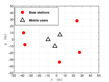
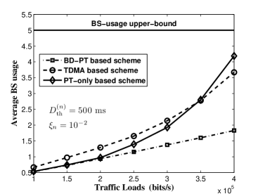
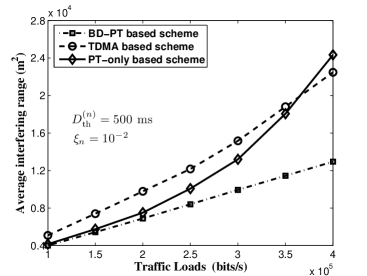
  (a)                                                   (b)                                                   (c)

Figure 4: (a) The deployment of BS’s and the positions of mobile users, where $K_{\mathrm{mu}}=3$ and $K_{\mathrm{bs}}=5$. (b) Simulation results of the average BS usage $\overline{L}$ versus traffic load under the specified delay-QoS requirements, where $\xi_{n}=10^{-2}$ and $D_{\mathrm{th}}^{(n)}=500$ ms for all $n$; $M_{m}=3$; $\kappa=1$. (b) Simulation results of the average interfering range versus traffic load under the same system setup as in (b).

  

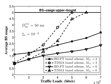
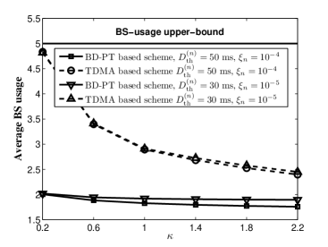
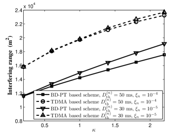
  (a)                                                   (b)                                                   (c)

Figure 5: (a) The average BS usage $\overline{L}$ versus traffic load under the specified delay-QoS requirements, where $D_{\mathrm{th}}^{(n)}=50$ ms, $\xi_{n}=10^{-4}$, and $N_{n}=2$ for all $n$; $\kappa=1$. (b) Average BS usage versus $\kappa$, where $M_{m}=5$. (c) Average interfering range versus $\kappa$, where the system setup is the same as in (b).

We use simulations to evaluate the performances of our proposed QoS-aware BS selection schemes for distributed MIMO links. The BS’s deployment and the mobile users’ positions are shown in Fig. 4(a), where $K_{\mathrm{bs}}=5$ and $K_{\mathrm{mu}}=3$. We set $T=10$ ms and $B=10^{5}$ Hz. We further assume that all users have the same number of receive antennas, all distributed BS’s have the same number of transmit antennas, and the incoming traffic loads for all users are equal. Furthermore, we employ the following average power propagation model. Specifically, the average received power gain $\overline{h}_{n,m}$ is equal to $G/d_{n,m}^{\eta}$, where $d_{n,m}$ is the distance between the $n$th mobile user and the $m$th BS, $G$ is a constant factor, and $\eta$ is the path loss exponent typically varying from 2 to 6 [13]. Without loss of generality, we let $\mathcal{P}_{\mathrm{ref}}=1$ and select $G$ such that $\overline{h}_{n,m}=0$ dB at $d_{n,m}=50$ m. Also, we set $\sigma_{\mathrm{th}}^{2}=0$ dB for evaluating of the average interfering range (see Section II-C).

Figures 4(b) and 4(c) compare the average BS usage and interfering range as functions of the incoming traffic load among our derived QoS-aware BS-selection schemes, including the joint BD-PT, TDMA, and PT-only based schemes. Fig. 4(b) shows that as the traffic load increases, all scheme’s average BS usages become larger to satisfy the more stringent QoS requirements. However, the TDMA and PT-only based schemes’ BS usages increase much more rapidly than our proposed BD-PT based scheme. This is because block diagonalization for multi-user MIMO communications can effectively take advantage of space multiplexing in removing the cross-interferences among all mobile users, and thus can achieve high spectral efficiency and system throughput. We can further observe that when the traffic load gets lower (larger), the PT-only based scheme needs less (more) BS’s to satisfy the specified QoS requirements, as compared to the TDMA based scheme. Fig. 4(c) plots the average interfering range caused by distributed MIMO transmissions, which displays the similar results to Fig. 4(b). This is expected because the total used power in each fading state linearly increases with the cardinality $L$ of selected BS-subset, as shown in Section II-D.

Figure 5(a) plots the average BS usage against traffic load with more stringent QoS constraints than the constraints used in Fig. 4(b). Under these more stringent constraints, the PT-only based scheme cannot support the specified QoS requirements for the incoming traffics and thus are not plotted in Fig. 5(a), which implies that the PT-only based scheme only works efficiently with loose QoS constraints. We can observe from Fig. 5(a) that the BD-PT based scheme generally outperforms the TDMA based scheme in terms of requiring fewer BS’s, especially when the traffic load is high. As shown in Fig. 5(a), for traffic load higher than or equal to 500 Kbits/s, the BS usage of the TDMA based scheme will reach the upper-bound, which is equal to $K_{\mathrm{bs}}$. This implies that all wireless resources have been used up while the specified QoS requirements for the incoming traffic still cannot be satisfied. In contrast, the BD-PT based scheme can clearly support even higher traffic load. An interesting observation is that the TDMA based scheme performs slightly better than the BD-PT based scheme, when the traffic load is low and the number of antennas per BS is small. This is because the advantage of BD technique can be effectively used when the spatial-multiplexing degree order is high. However, clearly the small number of transmit antennas can already successfully support smaller traffic load through TDMA strategy, while the BD in this case is not very effective due to the limited number of transmit antennas, implying insufficient freedom for spatial multiplexing.

Figures 5(b) and 5(c) depict the average BS usage and interfering range, respectively, versus the parameter $\kappa$, where $\kappa$ is defined in Section II-D, which is the power increasing rate with the number of BS’s selected for distributed MIMO transmissions. We can see that the average BS usage and the interfering range of the BD-PT based scheme are much smaller than those of the TDMA based scheme. As shown in Figs. 5(b) and 5(c), the lower delay bound and the smaller violation probability threshold, implying more stringent delay-QoS requirements, cause more BS usage and thus larger interfering range. This is because in order to satisfy more stringent QoS requirements, more BS’s need to get involved with the cooperative downlink transmissions to achieve the high system throughput for all mobile users. This also demonstrates that our proposed schemes can effectively adjust the transmission strategy to adapt to the specified QoS requirements. In addition, the average BS-usage is a decreasing function of $\kappa$ but the interfering range is an increasing function. This suggests that we can use more power to tradeoff the lower implementation complexity in distributed MIMO transmissions.

VII Conclusions

We proposed the QoS-aware BS-selection schemes for the distributed wireless MIMO links, which aim at minimizing the BS usages and reducing the interfering range, while satisfying diverse statistical delay-QoS constraints over multiple mobile users. In particular, we developed the joint block-diagonalization and probabilistic-transmission based scheme, the TDMA based scheme, and the pure probabilistic-transmission based scheme, respectively, to implement efficient BS-selection and the corresponding resource allocation algorithms for QoS provisioning of mobile users. Simulation results show that the joint block-diagonalization and probabilistic-transmission based scheme generally outperforms the TDMA based and pure probabilistic-transmission based schemes in terms of requiring less BS’s for data transmissions and decreasing the interfering range caused to the entire wireless networks. Moreover, the TDMA and probabilistic-transmission based schemes is efficient when the traffic load is not heavy.

References

• [1]
• [2] A. Sanderovich, S. Shamai (Shitz), and Y. Steinberg, “Distributed MIMO receiver–Achievable rates and upper bounds,” IEEE Trans. Inf. Theory, vol. 55, no. 10, pp. 4419-4438, Oct. 2009.
• [3] R-Mudumbai, D.R. Brown III, U. Madhow, and H.V. Poor, “Distributed transmit beamforming: Challenges and recent progress,” IEEE Commun. Mag., vol. 47, no. 2, pp. 102-110, Feb 2009.
• [4] P. Shang, G. Zhu, L. Tan, G. Su, and T. Li, “Transmit antenna selection for the distributed MIMO systems,” International Conference on Networks Security, Wireless Communications and Trusted Computing, 2009, pp. 449-453.
• [5] E. Telatar, “Capacity of multi-antenna Gaussian channels,” European Trans. Telecomm., vol. 10, no. 6, pp. 585-596, Nov. 1999.
• [6] S. Sanayei and A. Nosratinia, “Antenna selection in MIMO systems,” IEEE Commun. Mag., no. 10, pp. 68-73, October 2004.
• [7] M. Gharavi-Alkhansari, A. B. Gershman, “Fast antenna subset selection in MIMO systems,” IEEE Trans. Signal Processing, vol. 52, no. 2, pp. 339-347, Feb. 2004.
• [8] C.-S. Chang, Performance Guarantees in Communication Networks, Springer-Verlag London, 2000.
• [9] D. Wu and R. Negi, “Effective capacity: A wireless link model for support of quality of service,” IEEE Trans. on Wireless Commun., vol. 2, no. 4, July 2003, pp. 630-643.
• [10] X. Zhang, J. Tang, H.-H. Chen, S. Ci, and M. Guizni, “Cross-layer-based modeling for quality of service guarantees in mobile wireless networks,” IEEE Commun. Mag., pp. 100-106, Jan. 2006.
• [11] M. S. Bazaraa, H. D. Sherali, and C. M. Shetty, Nonlinear Programming: Theory and Algorithms, 3rd ed., John Wiley & Sons, Inc., 2006.
• [12] J. Tang and X. Zhang, “Quality-of-service driven power and rate adaptation over wireless links,” IEEE Trans. Wireless Commun., vol. 6, no. 8, pp. 3058-3068, Aug. 2007.
• [13] T. S. Rappaport, Wireless Communications: Principles & Practice, Prentice Hall, 1996.
• [14] H. Weingarten, Y. Steinberg and S. Shamai “The capacity region of the Gaussian multiple-input multiple-output broadcast channel,” IEEE Trans. Inf. Thoery, vol, 52, no. 9, pp. 3936-3964, Sep. 2006.
• [15] Q. H. Spencer, A. L. Swindlehurst, and M. Haardt, ”Zero-Forcing methods for downlink spatial multiplexing in multisuer MIMO channels,” IEEE Trans. Signal Processing, vol. 52, no. 2, Feb. 2004.
• [16] T. Yoo, A. Goldsmith, “On the Optimality of Multiantenna Broadcast Scheduling Using Zero-Forcing Beamforming,” IEEE J. Sel. Area Commun., vol. 24, no. 3, Mar. 2006, pp. 528-541.
• [17] S. Kaviani and W. A. Krzymien, “User Selection for Multiple-Antenna Broadcast Channel with Zero-Forcing Beamforming,” in Proc. IEEE GLOBECOM 2008, New Orleans, USA, Dec. 2008.
• [18] J. Tang and X. Zhang, “Cross-Layer-Model Based Adaptive Resource Allocation for Statistical QoS Guarantees in Mobile Wireless Networks,” IEEE Transactions on Wireless Communications, vol. 7, no. 6, pp. 2318–2328, June 2008.
• [19] Q. Du and X. Zhang, “Base-Station Selections for QoS Provisioning Over Distributed Multi-User MIMO Links in Wireless Networks,” Networking and Information Systems Labs., Dept. Electr. and Comput. Eng., Texas A&M Univ., College Station, Tech. Rep. [Online.] Available: http://www.ece.tamu.edu/$\sim$xizhang/papers/qos_bs_selection.pdf.