The Oxygen Abundance in the Solar Neighborhood

Abstract

We present a homogeneous analysis of the oxygen abundance in five H II regions and eight planetary nebulae (PNe) located at distances lower than 2 kpc and with available spectra of high quality. We find that both the collisionally excited lines and recombination lines imply that the PNe are overabundant in oxygen by about 0.2 dex. An explanation that reconciles the oxygen abundances derived with collisionally excited lines for H II regions and PNe with the values found for B-stars, the Sun, and the diffuse ISM requires the presence in H II regions of an organic refractory dust component that is not present in PNe. This dust component has already been invoked to explain the depletion of oxygen in molecular clouds and in the diffuse interstellar medium.

1. Introduction

The ionized gas that surrounds young stars in H II regions and evolved stars in planetary nebulae (PNe) is subjected to very similar processes, but the gas in H II regions samples the present interstellar medium (ISM), while the gas in PNe samples the ISM of several gigayears ago, when the progenitor stars formed. Hence, if we choose an element whose abundance in the PN has not changed significantly from the original one, like oxygen at near-solar metallicities (e.g., Karakas 2010), we can calculate its abundance in H II regions and PNe using the same procedure, and compare the differences with those predicted by galactic chemical evolution.

This potential is somewhat marred by the existing discrepancy between the abundances derived using collisionally excited lines (CELs) and those implied by recombination lines (RLs) of the same elements (Peimbert et al., 1993). In all the ionized nebulae studied so far, RLs imply abundances higher than those implied by CELs by factors around 2 in most cases, with some PNe showing much higher discrepancies (Liu, 2006). The emissivities of CELs have a stronger dependence on temperature than those of RLs, and most of the proposed explanations of the difference rely on the production of temperature fluctuations by some mechanism in the observed nebulae. The exception would be those explanations that consider uncertainties in the recombination coefficients of the heavy elements. The different explanations of the discrepancy imply that the real abundances will be either close to the values implied by CELs, closer to the abundances derived with RLs, or intermediate between them (Torres-Peimbert & Peimbert, 2003; Rodríguez & García-Rojas, 2010, and references therein). Therefore, a meaningful comparison between the abundances derived for H II regions and PNe must not only take into account the results provided by both CELs and RLs, but also the fact that the explanation can be different for the two kinds of objects.

A further issue to consider is that the ionizing radiation fields can be very different in H II regions and PNe. This implies that the corrections for the contribution of unobserved ions to the total abundance, generally based on the relative abundances of two ions of another element, are likely to introduce a different bias in each kind of object. Hence, the best option is to perform the comparison using an element whose dominant ionization states are all observed. In H II regions and low-ionization PNe, this happens with oxygen. Besides, the required [O II] and [O III] lines can be observed in the optical region of the spectrum along with the other H I and diagnostic lines needed for the analysis. This reduces the uncertainties introduced when comparing the relative intensities of lines measured at widely separated wavelengths, with mismatched apertures, and with different telescopes.

In this letter, we present a comparative analysis of the oxygen abundance in five H II regions and eight low-ionization PNe of the solar neighborhood. The solar neighborhood is defined here as a region around the Sun with a radius of 2 kpc. This allows us to secure a representative number of objects whose abundances should not be much affected by the Galactic abundance gradient. The analysis follows the same method and uses the same atomic data for all the objects. We use the best available spectra and provide results for both CELs and RLs. The derived oxygen abundances are compared with those implied by nearby young stars and those based on absorption lines in the diffuse ISM.

2. The sample

The sample objects were selected from the compilation in Delgado-Inglada et al. (2009) of Galactic H II regions and low ionization PNe with available deep optical spectra. There are around 100–800 detected lines in each object and the spectral resolution in the blue is better than 1.5 Å. All the objects have individual distance determinations locating them at distances below 2 kpc (see Section 3 below). The distance to NGC 6884 could be larger, but at a Galactic longitude of $82\deg$, the effect of the Galactic radial abundance gradient should be small.

The PNe have been classified as type II of Peimbert (Peimbert, 1978), though NGC 6210 could be of type III (Quireza et al., 2007). Quireza et al. estimate that the thin disk progenitors of type II PNe have ages around 4–6 Gyr and initial masses of 1.2–2.4 M_⊙.

3. Analysis and Results

We used the same set of lines for the analysis of all the sample objects. The lines were measured with the same telescope and aperture for each object. The physical conditions and ionic abundances were calculated with the nebular package in IRAF. In order to check the effect of the atomic data on the calculations, we performed two sets of calculations. The first set is based on the atomic data compiled in IRAF; the second one on the atomic data used in the photoionization code Cloudy (version 08.00, last described by Ferland et al. 1998). Below we present the results of the second set and comment on the differences found with the first one.

The adopted electron densities, $n_{\mathrm{e}}$, are weighted averages of the values implied by the diagnostics [S II] $\lambda 6716/\lambda 6731$, [Cl III] $\lambda 5517/\lambda 5537$, and [Ar IV] $\lambda 4711/\lambda 4740$. For M17 and the lower ionization objects we do not use the last diagnostic. In M17 the intensity of [Ar IV] $\lambda 4740$ is very uncertain and the intensity ratio $\lambda 4711/\lambda 4740$ is out of bounds; in M16 and M20 [Ar IV] $\lambda 4740$ was not measured; in IC 418, the [Ar IV] line ratio implies $n_{\mathrm{e}}=4800$ cm^-3, in disagreement with the other diagnostics, based on lines whose intensities in this object are larger by factors $\geq 50$. We derive two values for the electron temperature, $T_{\mathrm{e}}$, one for the high-ionization regions in the nebulae, $T_{\mathrm{e}}$([O III]), based on the ratio of line intensities $(\lambda 4959+\lambda 5007)/\lambda 4363$; another for the low-ionization regions, $T_{\mathrm{e}}$([N II]), based on $(\lambda 6548+\lambda 6583)/\lambda 5755$. We list in Table 3 the physical conditions derived for each object. We also give the observational uncertainties, i.e., those derived from the propagation of errors in the line intensities.

Table 1Physical Conditions

Object	$n_{\mathrm{e}}$([S II])	$n_{\mathrm{e}}$([Cl III])	$n_{\mathrm{e}}$([Ar IV])	$n_{\mathrm{e}}$(adopted)	$T_{\mathrm{e}}$([N II])	$T_{\mathrm{e}}$([O III])	ref
	(cm-3)	(cm-3)	(cm-3)	(cm-3)	(K)	(K)
H II regions
M8 (catalog )	$1500\pm 200$	$2000^{+400}_{-300}$	$2000^{+6700}_{-2000}$	$1600\pm 200$	$8500\pm 100$	$8000\pm 100$	1
M16 (catalog )	$1300^{+300}_{-200}$	$1300^{+700}_{-600}$	$\cdots$	$1300\pm 200$	$8500^{+100}_{-200}$	$7600^{+100}_{-200}$	2
M17 (catalog )	00$500^{+200}_{-100}$	00$200^{+400}_{-200}$	$\cdots$	00$400\pm 100$	$9200^{+200}_{-300}$	$7900\pm 100$	1
M20 (catalog )	00$300\pm 100$	00$300^{+500}_{-300}$	$\cdots$	00$300\pm 100$	$8500^{+100}_{-200}$	$7700^{+300}_{-200}$	2
M42 (catalog )	$5400^{+3700}_{-1700}$	$8000^{+700}_{-600}$	$4900^{+1100}_{-900}$	$7000\pm 500$	$10100^{+200}_{-300}$	$8250\pm 40$	3
Planetary Nebulae
IC 418 (catalog )	$16400^{+}_{-10600}$	$13400^{+5600}_{-3500}$	$\cdots$	$13900\pm 4200$	$8900^{+700}_{-600}$	$8700^{+400}_{-200}$	4
NGC 3132 (catalog )	00$500^{+200}_{-100}$	00$800^{+500}_{-400}$	00$300^{+600}_{-300}$	00$500\pm 100$	$9700^{+300}_{-200}$	$9400^{+200}_{-100}$	5
NGC 3242 (catalog )	$2100^{+600}_{-400}$	$1300^{+600}_{-500}$	$2100^{+800}_{-600}$	$1800\pm 300$	$12400^{+1800}_{-1100}$	$11600^{+300}_{-200}$	5
NGC 6210 (catalog )	$3700^{+1400}_{-900}$	$4100^{+900}_{-800}$	$6200^{+1100}_{-1000}$	$4600\pm 600$	$11200^{+400}_{-300}$	$9500\pm 200$	6
NGC 6543 (catalog )	$5800^{+7400}_{-2300}$	$6400^{+5200}_{-2700}$	$3100^{+1800}_{-1300}$	$3700\pm 1400$	$10300\pm 500$	$7800\pm 200$	7
NGC 6572 (catalog )	$16000^{+33000}_{-6800}$	$20100^{+4000}_{-2900}$	$15100^{+2200}_{-1900}$	$16400\pm 1800$	$12000^{+600}_{-500}$	$10200^{+300}_{-200}$	6
NGC 6720 (catalog )	00$500^{+200}_{-100}$	00$500^{+500}_{-400}$	00$700^{+600}_{-500}$	00$500\pm 100$	$10600\pm 300$	$10400^{+300}_{-200}$	6
NGC 6884 (catalog )	$6700^{+4100}_{-2000}$	$6800^{+1400}_{-1000}$	$9700^{+1600}_{-1300}$	$7900\pm 900$	$11600^{+400}_{-300}$	$10900^{+200}_{-300}$	6

References. — Line intensities from: (1) García-Rojas et al. (2007), (2) García-Rojas et al. (2006), (3) Esteban et al. (2004), (4) Sharpee et al. (2003), (5) Tsamis et al. (2003), (6) Liu et al. (2004a), (7) Wesson & Liu (2004).

The $\mbox{O}^{+}/\mbox{H}^{+}$ abundance ratio was calculated using the values found for $n_{\mathrm{e}}$, $T_{\mathrm{e}}$[N II] and $I(\mbox{[{O~{}II}]}~{}\lambda 3727)/I(\mbox{H}\beta)$; for the $\mbox{O}^{++}/\mbox{H}^{+}$ ratio we used $n_{\mathrm{e}}$, $T_{\mathrm{e}}$[O III] and $I(\mbox{[{O~{}III}]}~{}\lambda\lambda 4959,5007)/I(\mbox{H}\beta)$. The total oxygen abundance, (O/H)_CELs, was derived by adding up the O⁺ and O⁺⁺ abundances, and using ionization correction factors (ICFs) based on the He⁺⁺/He⁺ abundance ratio that provide estimates for the contribution of ions of higher degree of ionization (Kingsburgh & Barlow, 1994). Table 3 lists the Galactic coordinates and distances, $d$, to the objects, the ionic and total oxygen abundances, and the values used for the ICF (i.e., O/(O⁺+O⁺⁺), see Delgado-Inglada et al. 2009).

Table 3 also lists the results implied by RLs. The O⁺⁺ abundances were derived using the O II RLs of multiplet 1 (the only one measured in all the objects) and the recombination coefficients of Storey (1994). The multiplet intensity was calculated correcting for the unobserved lines, when necessary, using the prescriptions given by Peimbert et al. (2005). A comparison with the results obtained in the original references, that use all reliable multiplets, shows small differences in most cases, with a maximum difference of 0.14 dex. We estimated the total oxygen abundance implied by RLs, (O/H)_RLs, by assuming the same ionization fractions found with CELs.

Table 2Galactic Coordinates, Distances, and Chemical Abundances: $\{X^{+i}\}=12+\log(X^{+i}/\mathrm{H}^{+}$), $\{X\}=12+\log(X/\mathrm{H}$)

Object	$l(\arcdeg)$	$b(\arcdeg)$	$d$(kpc)	ref	{O${}^{+}\}_{\mathrm{CELs}}$	{O${}^{++}\}_{\mathrm{CELs}}$	ICF	{O}CELs	{O${}^{++}\}_{\mathrm{RLs}}$	{O}RLs
H II regions
M8 (catalog )	006	$-1$	1.322	1	$8.30\pm 0.04$	$7.90\pm 0.02$	$1.00$	$8.45\pm 0.03$	$8.24$	$8.79$
M16 (catalog )	17	$+1$	1.719	1	$8.41^{+0.05}_{-0.03}$	$7.93^{+0.05}_{-0.03}$	$1.00$	$8.53^{+0.04}_{-0.02}$	$8.31$	$8.91$
M17 (catalog )	15	$-1$	1.814	1	$7.70^{+0.07}_{-0.05}$	$8.47\pm 0.03$	$1.00$	$8.54\pm 0.02$	$8.73$	$8.82$
M20 (catalog )	007	00$0$	0.816	1	$8.40^{+0.05}_{-0.03}$	$7.76^{+0.05}_{-0.07}$	$1.00$	$8.49^{+0.04}_{-0.03}$	$8.08$	$8.82$
M42 (catalog )	209	$-19$	0.399	1	$7.77^{+0.06}_{-0.04}$	$8.45\pm 0.01$	$1.00$	$8.53\pm 0.01$	$8.61$	$8.68$
Planetary Nebulae
IC 418 (catalog )	215	$-24$	1.3	2	$8.53^{+0.18}_{-0.19}$	$8.11^{+0.05}_{-0.08}$	$1.00$	$8.67^{+0.14}_{-0.13}$	$8.21$	$8.81$
NGC 3132 (catalog )	272	$+12$	0.77	3	$8.38^{+0.05}_{-0.06}$	$8.55^{+0.02}_{-0.04}$	$1.02$	$8.78^{+0.02}_{-0.03}$	$8.81$	$9.03$
NGC 3242 (catalog )	261	$+32$	0.55	4	$6.45^{+0.15}_{-0.19}$	$8.45^{+0.03}_{-0.04}$	$1.18$	$8.53^{+0.03}_{-0.04}$	$8.85$	$8.93$
NGC 6210 (catalog )	43	$+38$	1.57	5	$7.16^{+0.05}_{-0.07}$	$8.66\pm 0.04$	$1.01$	$8.68\pm 0.04$	$9.01$	$9.02$
NGC 6543 (catalog )	96	$+30$	1.55	4	$7.10\pm 0.11$	$8.79\pm 0.05$	$1.00$	$8.80\pm 0.05$	$9.08$	$9.09$
NGC 6572 (catalog )	35	$+12$	1.49	5	$7.38^{+0.07}_{-0.09}$	$8.61^{+0.04}_{-0.05}$	$1.00$	$8.64^{+0.03}_{-0.05}$	$8.75$	$8.77$
NGC 6720 (catalog )	63	$+14$	0.704	6	$8.18\pm 0.05$	$8.52^{+0.03}_{-0.05}$	$1.12$	$8.73^{+0.02}_{-0.04}$	$8.88$	$9.09$
NGC 6884 (catalog )	82	$+7$	1.56,3.3	7,4	$7.11^{+0.05}_{-0.07}$	$8.58^{+0.04}_{-0.03}$	$1.13$	$8.65\pm 0.04$	$9.00$	$9.07$

References. — (1) Kharchenko et al. (2005), (2) Guzmán et al. (2009), (3) Ciardullo et al. (1999), (4) Mellema (2004), (5) Hajian et al. (1995), (6) Harris et al. (2007), (7) Palen et al. (2002).

The total oxygen abundances derived using the atomic data compiled in IRAF differ from those shown in Table 3 by a maximum of 0.05 dex with one exception, IC 418. For this nebula, the value implied by IRAF is $\sim 0.2$ dex higher. This large difference arises because the nebula has a high density and because its oxygen abundance is dominated by O⁺. When the electron density is high, the absolute uncertainties in $T_{\mathrm{e}}$([N II]) and $n_{\mathrm{e}}$ are large, and since the estimated O⁺ abundance is very sensitive to the physical conditions, its value is subject to large fluctuations.

In fact, as pointed out by the referee, the values of $T_{\mathrm{e}}$([N II]) are usually affected by many uncertainties, and this could be critical for our purposes. The [N II] diagnostic ratio is very susceptible to errors in the flux calibration and reddening correction, and can be altered by a contribution from recombination to [N II] $\lambda 5755$ (Rubin, 1986), or by contamination from high-density objects included in the slit, like cometary knots, globules, proplyds, or Herbig-Haro objects (e.g., Mesa-Delgado et al., 2008). The recombination contribution can be large for objects with high degrees of ionization, but for these objects O⁺ makes a small contribution to the total abundance, which is then barely affected. On the other hand, the contamination by high-density objects could be a problem for the sample PNe, since most of them were observed using a long-slit scanning all of their volume. Our sample H II regions are less likely to be contaminated, since they were observed using small slits ($\sim 3^{\prime\prime}\times 10^{\prime\prime}$), and include nebulae like M42, the Orion Nebula, where proplyds and Herbig-Haro objects are easily resolved and identified. The uncertainties in $T_{\mathrm{e}}$([N II]) have prompted some authors to use only $T_{\mathrm{e}}$([O III]) to calculate all the ionic abundances. If we did this, the oxygen abundances would be higher by up to 0.03 dex in our PNe, and by significant amounts, $0.07\mbox{--}0.20$ dex, in the H II regions: $12+\log(\mathrm{O}/\mathrm{H})^{\prime}_{\mathrm{CELs}}=8.55$, 8.73, 8.61, 8.68, and 8.64 for M8, M16, M17, M20, and M42, respectively. However, we consider that the evidence for the values of $T_{\mathrm{e}}$([N II]) shown in Table 3 is strong, in particular for the H II regions. Temperature values similar to those presented here and also satisfying $T_{\mathrm{e}}$([N II]) $>T_{\mathrm{e}}$([O III]) are generally found at different positions within the bright areas of our sample H II regions (e.g., Rodríguez, 1999; Mesa-Delgado et al., 2008). These temperature gradients are also predicted by photoionization models (Stasińska, 1978). Furthermore, the temperatures and temperature ratios measured for the sample H II regions from the same spectra we are using here have been shown to be consistent with the predictions of photoionization models (Rodríguez & García-Rojas, 2010). We conclude that the available evidence indicates that our values of $T_{\mathrm{e}}$([N II]) are reliable, but problems with this temperature could be a possible source of bias when comparing abundances in H II regions and PNe.

The presence of unresolved high-density regions in the observed volumes might also introduce a bias in our results by affecting in different ways the CELs we are using (Rubin, 1989). Recently, Tsamis et al. (2011) have argued that small high-density clumps are seriously affecting the intensities of CELs in H II regions, thus producing the discrepancy between CELs and RLs in these nebulae. However, both the fact that different density diagnostics imply very similar densities in the sample H II regions (Esteban et al., 2004; García-Rojas et al., 2006, 2007) and the success of constant-density photoionization models in reproducing the intensities of the main CELs involved in the determination of electron temperatures and oxygen abundances in these objects (Rodríguez & García-Rojas, 2010) suggest that high-density clumps, if present, have only a small effect on the spectra of our sample H II regions.

If we now compare our results with those derived by other authors from the same spectra (see Tsamis et al. 2004 and Liu et al. 2004b, in addition to the references listed in Table 3), the differences are larger, since besides using different atomic data, they use other lines. The differences are all $\lesssim 0.1$ dex with three exceptions: Sharpee et al. (2004) find (O/H)_CELs 0.21 dex below our value in IC 418, whereas Tsamis et al. (2003) and Wesson & Liu (2004) find (O/H)_RLs 0.17 and 0.21 dex above our derived values for NGC 3132 and NGC 6543, respectively.

Finally, we note the importance of using spectra of relatively high spectral resolution in order to obtain the best estimates for the oxygen abundance, even when using strong CELs. If the spectral resolution is poor, [O III] $\lambda 4363$ can be blended with several lines, like [Fe II] $\lambda 4359$, O II $\lambda 4367$, and O I $\lambda 4368$. In the sample H II regions, these blends would lead to values of $T_{\mathrm{e}}$([O III]) up to 1000 K higher and final oxygen abundances up to 0.05 dex lower. In our sample PNe the effects are smaller: up to 300 K higher $T_{\mathrm{e}}$([O III]) and oxygen abundances up to 0.02 dex lower.

4. Discussion

Figure 1 shows the total oxygen abundances implied by CELs and RLs for the H II regions and PNe as a function of $\mbox{O}^{+}/\mbox{O}^{++}$. All the H II regions show similar abundances, with $12+\langle\log(\mathrm{O}/\mathrm{H})_{\mathrm{CELs}}\rangle_{\mathrm{H~{}II}}=8.52$ and $12+\langle\log(\mathrm{O}/\mathrm{H})_{\mathrm{RLs}}\rangle_{\mathrm{H~{}II}}=8.80$, suggesting that the ISM in the solar neighborhood is homogeneous. The PNe results show more dispersion, but can be seen to be higher by about 0.2 dex: $12+\langle\log(\mathrm{O}/\mathrm{H})_{\mathrm{CELs}}\rangle_{\mathrm{PNe}}=8.70$ and $12+\langle\log(\mathrm{O}/\mathrm{H})_{\mathrm{RLs}}\rangle_{\mathrm{PNe}}=8.98$. We expect to find the real oxygen abundances of the nebulae somewhere in the ranges defined by CELs and RLs, with the different explanations of the discrepancy favoring values at different positions along these ranges. There are some indications that the explanations might differ in H II regions and PNe, like the fact that all the H II regions studied so far show moderate discrepancies, whereas PNe can show huge discrepancies, like NGC 1501, where Ercolano et al. (2004) find $12+\log(\mathrm{O}/\mathrm{H})_{\mathrm{CELs}}=8.52$ and $12+\log(\mathrm{O}/\mathrm{H})_{\mathrm{RLs}}=10.09$. However, at least three of the PNe show CELs abundances similar to the RLs abundances of the H II regions. This implies that even if the explanation of the abundance discrepancy is very different in each kind of object, these PNe will still show similar or larger oxygen abundances than the H II regions. This is contrary to our expectations from simple models of galactic chemical evolution. The difference could arise from extensive stellar migration from the inner parts of the Galaxy, or gas flows or infall (e.g., Schönrich & Binney, 2009). An overabundance of oxygen in PNe could also arise from oxygen production in the stellar progenitors, although this is not expected to be significant at near-solar metallicities (e.g., Marigo, 2001; Karakas, 2010).

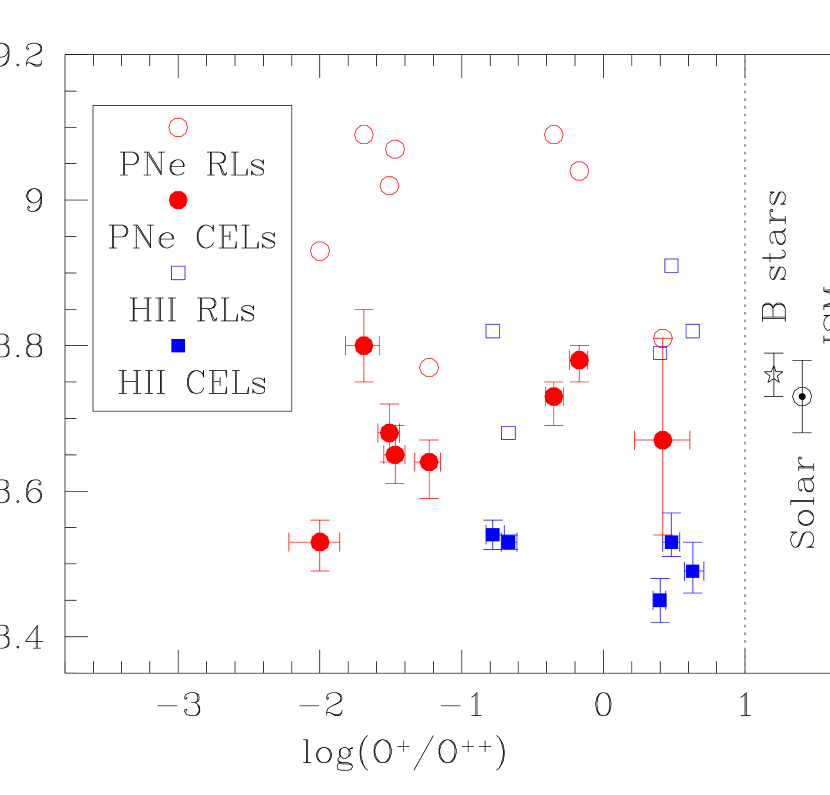
Figure 1.— Oxygen abundances derived using CELs (filled circles and squares) and RLs (empty circles and squares) for our sample H II regions (squares) and PNe (circles) as a function of the values of $\mbox{O}^{+}/\mbox{O}^{++}$. From left to right, the objects are: NGC 3242, NGC 6543, NGC 6210, NGC 6884, NGC 6572, M17, M42, NGC 6720, NGC 3132, M8, IC 418, M16, and M20. We also show the protosolar abundance (the symbol $\sun$, Asplund et al., 2009), the abundance of nearby B stars (star, Przybilla et al., 2008), and the range of abundances found for the ISM (rectangle, Jenkins, 2009).

In order to shed light on this issue, Figure 1 also shows the protosolar abundance of Asplund et al. (2009), the results obtained for several nearby B stars by Przybilla et al. (2008), and the range of values found for the diffuse ISM by Jenkins (2009). We will assume that these results, which can be considered as representative of the best estimates for these objects, are not affected by important systematic errors and we will try to find a way to reconcile our results with them.

The RLs abundances of H II regions are similar to the B-star values, but their discrepancy with the abundances implied by CELs might be difficult to justify, especially if one must look for a mechanism that operates in H II regions but not in PNe. One possibility is suggested by the different sensitivity of the calculated values of (O/H)_CELs in H II regions and PNe to changes in the assumed temperature structure (see Section 3): temperature fluctuations in a chemically homogeneous medium could be responsible for the discrepancy in H II regions (supporting the RLs abundances in these nebulae, see, e.g., Esteban et al. 2004), whereas some kind of metal-rich inclusions could produce the discrepancy in PNe (supporting the CELs abundances in these objects, e.g., Liu et al., 2000; Henney & Stasińska, 2010). However, all these explanations have problems, related to the origin and survival of the metal-rich inclusions or to the nature of the mechanism responsible for the temperature fluctuations (Liu et al., 2000; Henney & Stasińska, 2010; Rodríguez & García-Rojas, 2010, and references therein). We explore below an alternative explanation.

The abundances implied by CELs in H II regions are too low, except when compared with the lower values found in the ISM. The oxygen abundances derived by Jenkins (2009) for the ISM follow a trend with the overall amount of depletion implied by all observed elements, suggesting that the different values represent different amounts of depletion onto dust grains. Could the low abundances in H II regions be due to their having a larger fraction of oxygen deposited in dust grains?

Dust grains in PNe and H II regions should have different characteristics, consisting of recently created stardust in PNe, and heavily processed interstellar grains in H II regions. However, the amount of oxygen that can be in grains outside of molecular clouds is limited by the availability of atoms of those elements that bind to oxygen to form refractory compounds like oxides and silicates. Whittet (2010) estimates that a maximum of 90–140 ppm of oxygen can be located in silicates and oxides. A correction for this amount would increase the value of $12+\langle\log(\mathrm{O}/\mathrm{H})_{\mathrm{CELs}}\rangle_{\mathrm{H~{}II}}$ to a maximum of 8.67, close to $12+\langle\log(\mathrm{O}/\mathrm{H})_{\mathrm{CELs}}\rangle_{\mathrm{PNe}}$, but at least some of the PNe (NGC 6210 and NGC 6543) might need similar corrections, since they harbor oxygen-rich dust like the H II regions (Bernard-Salas & Tielens 2005; Delgado-Inglada & Rodríguez, in preparation).

In fact, Jenkins (2009) finds that the highest levels of oxygen depletion (the lowest abundance values) cannot be explained with depletion in silicates and oxides, and concludes that oxygen must be locked up with an element as abundant as hydrogen or carbon. Whittet (2010) points out that a similar shortfall of oxygen (around 160 ppm) is observed in molecular clouds, and argues that the most plausible explanation involves an organic refractory dust component arising from the irradiation of ices by UV photons in molecular clouds. This component would not be expected to be present in PNe. So, is the missing oxygen in H II regions deposited in cometary-like dust grains?

Correcting the oxygen abundances implied by CELs in H II regions by 160 ppm (for the oxygen in the organic refractory component) and 115 ppm (as an estimate for the oxygen in silicates and oxides), we get $12+\langle\log(\mathrm{O}/\mathrm{H})_{\mathrm{CELs}}\rangle_{\mathrm{H~{}II}}=8.78$, in agreement with the B-stars abundances. This value also agrees with the values implied by CELs in PNe, even if they are corrected for the presence of silicates and oxides. The latter agreement is what one would expect from the almost flat age-metallicity relation followed by nearby F and G stars (e.g., Holmberg et al., 2009), though the relatively small dispersion in the abundances derived for our PNe suggests that the spread of stellar metallicities at a given age should be smaller than what is usually considered.

In order to confirm our interpretation or to distinguish between other possibilities, homogeneous comparisons of the abundances of other elements would be valuable. Note, however, that they would require studying the bias introduced by the ICFs and whether it is different in H II regions and PNe.

5. Conclusions

We have selected a sample of five H II regions and eight low-ionization PNe that have available spectra of high quality, all of them located at distances lower than 2 kpc. A homogeneous analysis of their oxygen abundances based on CELs and RLs shows that the PNe are, on average, overabundant by 0.18 dex.

If we take at face value the results implied by B-stars, the Sun, and the diffuse ISM, along with the almost flat age-metallicity relation implied by F and G stars, we find that for the PNe, the abundances implied by CELs agree with the expected values, whereas the abundances implied by RLs are too high. For the H II regions, the abundances implied by CELs are similar to the lower values found by Jenkins (2009) in the ISM, which are explained by Whittet (2010) as due to depletion in organic refractory dust grains. If we assume that these grains are also present in H II regions, their CELs abundances agree with all the other results. We can thus explain the overabundance of oxygen in PNe through the presence of different dust components in H II regions and PNe.

References

- Asplund et al. (2009) Asplund, M., Grevesse, N., Sauval, A. J., & Scott, P. 2009, ARA&A, 47, 481
- Bernard-Salas & Tielens (2005) Bernard-Salas, J., & Tielens, A. G. G. M. 2005, A&A, 431, 523
- Ciardullo et al. (1999) Ciardullo, R., Bond, H. E., Sipior, M. S., Fullton, L. K., Zhang, C.-Y., & Schaefer, K. G. 1999, AJ, 118, 488
- Delgado-Inglada et al. (2009) Delgado-Inglada, G., Rodríguez, M., Mampaso, A., & Viironen, K. 2009, ApJ, 694, 1335
- Ercolano et al. (2004) Ercolano, B., Wesson, R., Zhang, Y., Barlow, M. J., De Marco, O., Rauch, T., & Liu, X.-W. 2004, MNRAS, 354, 558
- Esteban et al. (2004) Esteban, C., Peimbert, M., García-Rojas, J., Ruiz, M.-T., Peimbert, A., & Rodríguez, M. 2004, MNRAS, 355, 229
- Ferland et al. (1998) Ferland, G. J., Korista, K. T., Verner, D. A., Ferguson, J. W., Kingdon, J. B., & Verner, E. M. 1998, PASP, 110, 761
- García-Rojas et al. (2006) García-Rojas, J., Esteban, C., Peimbert, M., Costado, M. T., Rodríguez, M., Peimbert, A., & Ruiz, M.-T. 2006, MNRAS, 368, 253
- García-Rojas et al. (2007) García-Rojas, J., Esteban, C., Peimbert, A., Rodríguez, M., Peimbert, M., & Ruiz, M.-T. 2007, Rev. Mexicana Astron. Astrofis., 43, 3
- Guzmán et al. (2009) Guzmán, L., Loinard, L., Gómez, Y., & Morisset, C. 2009, AJ, 138, 46
- Hajian et al. (1995) Hajian, A. R., Terzian, Y., & Bignell, C. 1995, AJ, 109, 2600
- Harris et al. (2007) Harris, H. C., Dahn, C. C., Canzian, B., et al. 2007, AJ, 133, 631
- Henney & Stasińska (2010) Henney, W. J. & Stasińska, G. 2010, ApJ, 711, 881
- Holmberg et al. (2009) Holmberg, J., Nordström, B., & Andersen, J. 2009, A&A, 501, 941
- Jenkins (2009) Jenkins, E. B. 2009, ApJ, 700, 1299
- Karakas (2010) Karakas, A. I. 2010, MNRAS, 403, 1413
- Kharchenko et al. (2005) Kharchenko, N. V., Piskunov, A. E., Röser, S., Schilbach, E., & Scholz, R.-D. 2005, A&A, 438, 1163
- Kingsburgh & Barlow (1994) Kingsburgh, R. L. & Barlow, M. J. 1994, MNRAS, 271, 257
- Liu (2006) Liu, X.-W. 2006, in IAU Symp. 234, Planetary Nebulae in our Galaxy and Beyond, ed. M. J. Barlow & R. H. Méndez (Cambridge: Cambridge University Press), 219
- Liu et al. (2000) Liu, X.-W., Storey, P. J., Barlow, M. J., Danziger, I. J., Cohen, M., & Bryce, M. 2000, MNRAS, 312, 585
- Liu et al. (2004a) Liu, Y., Liu, X.-W., Barlow, M. J., & Luo, S.-G. 2004a, MNRAS, 353, 1251
- Liu et al. (2004b) Liu, Y., Liu, X.-W., Luo, S.-G., & Barlow, M. J. 2004b, MNRAS, 353, 1231
- Marigo (2001) Marigo, P. 2001, A&A, 370, 194
- Mellema (2004) Mellema, G. 2004, A&A, 416, 623
- Mesa-Delgado et al. (2008) Mesa-Delgado, A., Esteban, C., & García-Rojas, J. 2008, ApJ, 675, 389
- Palen et al. (2002) Palen, S., Balick, B., Hajian, A. R., Terzian, Y., Bond, H. E., & Panagia, N. 2002, AJ, 123, 2666
- Peimbert et al. (2005) Peimbert, A., Peimbert, M., & Ruiz, M.-T. 2005, ApJ, 634, 1056
- Peimbert (1978) Peimbert, M. 1978, in IAU Symp. 76, Planetary Nebulae, Observation and Theory, ed. Y. Terzian (Dordrecht: Reidel), 215
- Peimbert et al. (1993) Peimbert, M., Storey, P. J., & Torres-Peimbert, S. 1993, ApJ, 414, 626
- Przybilla et al. (2008) Przybilla, N., Nieva, M. F., & Butler, K. 2008, ApJ, 688, L103
- Quireza et al. (2007) Quireza, C., Rocha-Pinto, H. J., & Maciel, W. J. 2007, A&A, 475, 217
- Rodríguez (1999) Rodríguez, M. 1999, A&A, 351, 1075
- Rodríguez & García-Rojas (2010) Rodríguez, M., & García-Rojas, J. 2010, ApJ, 708, 1551
- Rubin (1986) Rubin, R. H. 1986, ApJ, 309, 334
- Rubin (1989) Rubin, R. H. 1989, ApJS, 69, 897
- Schönrich & Binney (2009) Schönrich, R., & Binney, J. 2009, MNRAS, 396, 203
- Sharpee et al. (2003) Sharpee, B., Williams, R., Baldwin, J. A., & van Hoof, P. A. M. 2003, ApJS, 149, 157
- Sharpee et al. (2004) Sharpee, B., Baldwin, J. A., & Williams, R. 2004, ApJ, 615, 323
- Stasińska (1978) Stasińska, G. 1978, A&AS, 32, 429
- Storey (1994) Storey, P. J. 1994, A&A, 282, 999
- Torres-Peimbert & Peimbert (2003) Torres-Peimbert, S., & Peimbert, M. 2003, in IAU Symp. 209, Planetary Nebulae: Their Evolution and Role in the Universe, ed. S. Kwok, M. Dopita, & R. Sutherland (San Francisco: ASP), 363
- Tsamis et al. (2003) Tsamis, Y. G., Barlow, M. J., Liu, X.-W., Danziger, I. J., & Storey, P. J. 2003, MNRAS, 345, 186
- Tsamis et al. (2004) Tsamis, Y. G., Barlow, M. J., Liu, X.-W., Storey, P. J., & Danziger, I. J. 2004, MNRAS, 353, 953
- Tsamis et al. (2011) Tsamis, Y. G., Walsh, J. R., Vílchez, J. M., & Péquignot, D. 2011, MNRAS, 412, 1367
- Wesson & Liu (2004) Wesson, R. & Liu, X.-W. 2004, MNRAS, 351, 1026
- Whittet (2010) Whittet, D. C. B. 2010, ApJ, 710, 1009