A test of significance in functional quadratic regression

Abstract

We consider a quadratic functional regression model in which a scalar response depends on a functional predictor; the common functional linear model is a special case. We wish to test the significance of the nonlinear term in the model. We develop a testing method which is based on projecting the observations onto a suitably chosen finite dimensional space using functional principal component analysis. The asymptotic behavior of our testing procedure is established. A simulation study shows that the testing procedure has good size and power with finite sample sizes. We then apply our test to a data set provided by Tecator, which consists of near-infrared absorbance spectra and fat content of meat.

and

1 Introduction and results

In a predictive model, it may be more natural and appropriate for certain quantities to be represented as trajectories rather than a single number (Kirkpatrick and Heckman [16]). For example, a young animal’s size may be considered as a function of time, giving a growth trajectory. A model to predict a certain response from growth trajectories is useful to animal breeders because they may be able to produce more valuable animals by changing their growth patterns (Fitzhugh [12]). Müller and Zhang [19] used egg-laying trajectories from Mediterranean fruit flies to predict a female fly’s remaining lifetime. Frank and Friedman [13] and Wold [23] provide an early discussion on the applications of principal components to analyze curves in chemistry. Further examples for analysis of data when the observations are curves can be found in Fan and Lin [8], Laukaitis and Račkauskas [17], Cardot et al. [5] and Zhang and Chen [25]. For surveys on functional data analysis, we refer to the books of Ferraty and Vieu [10], Ferraty and Romain [9] and Horváth and Kokoszka [15].

Yao and Müller [24] and Borggaard and Thodberg [1] used absorbance trajectories to predict the fat content of meat samples. The absorbance at any particular wavelength is a measurement related to the proportion of light that passes through a meat sample. A representative sample of 15 of the 240 absorbance trajectories are pictured in Figure 1.

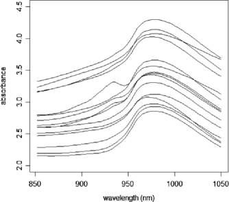
Figure 1: Absorbance trajectories from 15 samples of finely chopped pure meat.

In functional regression, special attention has been given to functional linear models (Cardot et al. [4], Shen and Faraway [22], Cai and Hall [3], Hall and Horowitz [14]). However, it is pointed out in Yao and Müller [24] that this model imposes a constraint on the regression relationship that may not be appropriate in some scenarios. Yao and Müller [24] generalized this to a functional polynomial model, which has greater flexibility. In functional polynomial regression, as in standard polynomial regression, one must balance the costs and benefits of using more parameters in the model. In this paper, we will develop a test to determine if a quadratic term is justified in the model or if a functional linear model adequately describes the regression relationship.

We assume that the predictor, $X_{n}(t)$, is defined on a finite interval which, without loss of generality, will be $[0,1]$. The functional quadratic model in which a scalar response, $Y_{n}$, is paired with a functional predictor, $X_{n}(t)$, is defined as

$$Y_{n}=\mu+\int_{0}^{1}k(t)X_{n}^{c}(t)\,\mathrm{d}t+\int_{0}^{1}\int_{0}^{1}h(s,t)X_{n}^{c}(s)X_{n}^{c}(t)\,\mathrm{d}t\,\mathrm{d}s+\varepsilon_{n},$$ (1)

where $X_{n}^{c}(t)=X_{n}(t)-E(X_{n}(t))$ is the centered predictor process and $\varepsilon_{n}$ is a random error. The functions $k(t)$ and $h(s,t)$ are regression parameter functions in the model (1). If $h(s,t)=0$, then $\mu=E(Y_{n})$ and (1) reduces to the functional linear model

$$Y_{n}=\mu+\int_{0}^{1}k(t)X_{n}^{c}(t)\,\mathrm{d}t+\varepsilon_{n}.$$ (2)

Yao and Müller [24] developed estimators for the functions $k$ and $h$ and prediction theory for the model (1). Cardot and Sarda [6] and Mas and Pumo [20] point out in their survey papers that since we can choose a function in (2), the functional linear model can be used in a large variety of applications. The functional linear model provides a very simple relation between $X_{n}(t)$ and $Y_{n}$, so it is important to check if the more involved quadratic model (1) provides a real improvement. In other words, one should test whether the quadratic term is really needed. To test the significance of the quadratic term in (1), we test the null hypothesis,

$$H_{0}\colon\ h(s,t)=0,$$ (3)

against the alternative

$$H_{A}\colon\ h(s,t)\neq 0.$$

To reduce the dimensionality and avoid overfitting in our functional regression model, we will project the predictor process onto a suitably chosen finite dimensional space. The space is spanned by the eigenfunctions of $C(t,s)=E(X_{n}(t)-\mu_{X}(t))(X_{n}(s)-\mu_{X}(s))$, the covariance function of the predictor process, where $\mu_{X}(t)=EX_{n}(t)$. We will denote the eigenfunctions and associated eigenvalues by $\{(v_{i}(t),\lambda_{i}),1\leq i\leq\infty\}$. We can and will assume that $\lambda_{i}$ is the $i$th largest eigenvalue and that the eigenfunctions are orthonormal. It is clear that we can assume that $h$ is symmetric, and we also impose the condition that the kernels are in $L^{2}$:

$$h(s,t) = h(t,s)\quad\mbox{and}\quad\int_{0}^{1}\int_{0}^{1}h^{2}(s,t)\,\mathrm{d}t\,\mathrm{d}s<\infty,$$ (4)

$$\int_{0}^{1}k^{2}(t)\,\mathrm{d}t < \infty.$$ (5)

Thus, we have the expansions

$$h(s,t) = \sum_{i=1}^{\infty}\sum_{j=1}^{\infty}a_{i,j}v_{j}(s)v_{i}(t)$$

$$= \sum_{i=1}^{\infty}a_{i,i}v_{i}(s)v_{i}(t)+\sum_{i=1}^{\infty}\sum_{j=i+1}^{\infty}a_{i,j}\bigl{(}v_{j}(s)v_{i}(t)+v_{i}(s)v_{j}(t)\bigr{)}$$

and

$$k(t)=\sum_{i=1}^{\infty}b_{i}v_{i}(t).$$ (7)

Let $\langle\cdot,\cdot\rangle$ denote the inner product in $L^{2}$. By projecting onto the space spanned by $\{v_{1},\dots,v_{p}\}$ and using (1) and (7), we can write the model (1) as

$$Y_{n}=\mu+\sum_{i=1}^{p}b_{i}\bigl{\langle}X_{n}^{c},v_{i}\bigr{\rangle}+\sum_{i=1}^{p}\sum_{j=i}^{p}\bigl{(}2-1\{i=j\}\bigr{)}a_{i,j}\bigl{\langle}X_{n}^{c},v_{i}\bigr{\rangle}\bigl{\langle}X_{n}^{c},v_{j}\bigr{\rangle}+\varepsilon_{n}^{*},$$ (8)

where

$$\varepsilon_{n}^{*} = \varepsilon_{n}+\sum_{i=p+1}^{\infty}b_{i}\bigl{\langle}X_{n}^{c},v_{i}\bigr{\rangle}+\sum_{i=p+1}^{\infty}\sum_{j=i}^{\infty}\bigl{(}2-1\{i=j\}\bigr{)}a_{i,j}\bigl{\langle}X_{n}^{c},v_{i}\bigr{\rangle}\bigl{\langle}X_{n}^{c},v_{j}\bigr{\rangle}$$

$${}+\sum_{i=1}^{p}\sum_{j=p+1}^{\infty}2a_{i,j}\bigl{\langle}X_{n}^{c},v_{i}\bigr{\rangle}\bigl{\langle}X_{n}^{c},v_{j}\bigr{\rangle}.$$

We note that (8) is written as a standard linear model, but the error term, $\varepsilon^{*}_{n}$, and the design points, $\{\langle X_{n}^{c},v_{i}\rangle,1\leq i\leq p\}$, are dependent.

We observe $(Y_{n},X_{n}(t),0\leq t\leq 1),1\leq n\leq N.$ Unfortunately, we cannot use (8) directly for statistical inference since $v_{i}(t)$ and $\mu_{X}(t)$ are unknown. We estimate $\mu_{X}(t)$ and $C(t,s)$ with the corresponding empiricals

$$\bar{X}(t)=\frac{1}{N}\sum_{n=1}^{N}X_{n}(t)$$

and

$$\hat{C}(t,s)=\frac{1}{N}\sum_{n=1}^{N}\bigl{(}X_{n}(t)-\bar{X}(t)\bigr{)}\bigl{(}X_{n}(s)-\bar{X}(s)\bigr{)}.$$

The eigenvalues and the corresponding eigenfunctions of $\hat{C}(t,s)$ are denoted by $\hat{\lambda}_{1}\geq\hat{\lambda}_{2}\geq\cdots$ and $\hat{v}_{1},\hat{v}_{2},\dots$ . Eigenfunctions corresponding to unique eigenvalues are uniquely determined up to signs. For this reason, we cannot expect more than to have $\hat{c}_{i}\hat{v}_{i}(t)$ be close to $v_{i}(t)$, where the $\hat{c}_{i}$’s are random signs. We replace equation (8) with

$$Y_{n} = \mu+\sum_{i=1}^{p}b_{i}\langle X_{n}-\bar{X},\hat{c}_{i}\hat{v}_{i}\rangle$$

$${}+\sum_{i=1}^{p}\sum_{j=i}^{p}\bigl{(}2-1\{i=j\}\bigr{)}a_{i,j}\langle X_{n}-\bar{X},\hat{c}_{i}\hat{v}_{i}\rangle\langle X_{n}-\bar{X},\hat{c}_{j}\hat{v}_{j}\rangle+\varepsilon_{n}^{**},$$

where

$$\varepsilon_{n}^{**} = \varepsilon_{n}^{*}+\sum_{i=1}^{p}b_{i}\bigl{\langle}X_{n}^{c},v_{i}-\hat{c}_{i}\hat{v}_{i}\bigr{\rangle}+\sum_{i=1}^{p}b_{i}\langle\bar{X}-\mu_{X},\hat{c}_{i}\hat{v}_{i}\rangle$$

$${}-\sum_{i=1}^{p}\sum_{j=i}^{p}\bigl{(}2-1\{i=j\}\bigr{)}a_{i,j}\bigl{(}\langle X_{n}-\bar{X},\hat{c}_{i}\hat{v}_{i}\rangle\langle X_{n}-\bar{X},\hat{c}_{j}\hat{v}_{j}\rangle-\bigl{\langle}X_{n}^{c},v_{i}\bigr{\rangle}\bigl{\langle}X_{n}^{c},v_{j}\bigr{\rangle}\bigr{)}.$$

We can write (1) in the concise form

$${\mathbf{Y}}=\hat{\mathbf{Z}}\pmatrix{\tilde{\mathbf{A}}\cr\tilde{\mathbf{B}}\cr\mu}+{\bm{\varepsilon}^{**}},$$ (10)

where

$${\mathbf{Y}} = (Y_{1},Y_{2},\dots,Y_{N})^{T}\in R^{N},$$

$$\tilde{\mathbf{A}} = \operatorname{vech}\bigl{(}\bigl{\{}\hat{c}_{i}\hat{c}_{j}a_{i,j}\bigl{(}2-1\{i=j\}\bigr{)},1\leq i\leq j\leq p\bigr{\}}^{T}\bigr{)}\in R^{p(p+1)/2},$$

$$\tilde{\mathbf{B}} = (\hat{c}_{1}b_{1},\hat{c}_{2}b_{2},\dots,\hat{c}_{p}b_{p})^{T}\in R^{p},\qquad{\bm{\varepsilon}}^{**}=\bigl{(}\varepsilon_{1}^{**},\varepsilon_{2}^{**},\dots,\varepsilon_{N}^{**}\bigr{)}^{T}\in R^{N},$$

and $\hat{{\mathbf{Z}}}$ is a $N\times(p(p+1)/2+p+1)$ matrix given by

$$\hat{{\mathbf{Z}}}=\pmatrix{\hat{\mathbf{D}}_{1}^{T}&\hat{\mathbf{F}}_{1}^{T}&1\cr\hat{\mathbf{D}}_{2}^{T}&\hat{\mathbf{F}}_{2}^{T}&1\cr\vdots&\vdots&\vdots\vspace*{3pt}\cr\hat{\mathbf{D}}_{N}^{T}&\hat{\mathbf{F}}_{N}^{T}&1}$$

with

$$\hat{\mathbf{D}}_{n} = \operatorname{vech}\bigl{(}\bigl{\{}\langle\hat{v}_{i},X_{n}-\bar{X}\rangle\langle\hat{v}_{j},X_{n}-\bar{X}\rangle,1\leq i\leq j\leq p\bigr{\}}^{T}\bigr{)}\in R^{p(p+1)/2},$$

$$\hat{\mathbf{F}}_{n} = \bigl{(}\langle X_{n}-\bar{X},\hat{v}_{1}\rangle,\langle X_{n}-\bar{X},\hat{v}_{2}\rangle,\dots,\langle X_{n}-\bar{X},\hat{v}_{p}\rangle\bigr{)}^{T}\in R^{p}.$$

The half-vectorization, $\operatorname{vech}(\cdot)$, stacks the columns of the lower triangular portion of the matrix under each other. Although we write our model in the form of a general linear model, it is important to note that it is not a classical linear model. First, ${\bm{\varepsilon}^{**}}$ is correlated with $\hat{\mathbf{Z}}$ because ${\bm{\varepsilon}^{**}}$ contains additional error terms which come from projecting onto a p-dimensional space. Another important difference between (10) and a classical linear model is that the parameters to be estimated, $\tilde{\mathbf{A}}$ and $\tilde{\mathbf{B}}$, are random; they depend on the random signs, $\hat{c}_{i}$. We estimate $\tilde{\mathbf{A}}$, $\tilde{\mathbf{B}}$, and $\mu$ using the least squares estimator:

$$\pmatrix{\hat{\mathbf{A}}\cr\hat{\mathbf{B}}\cr\hat{\mu}}=\bigl{(}\hat{\mathbf{Z}}^{T}\hat{\mathbf{Z}}\bigr{)}^{-1}\hat{\mathbf{Z}}^{T}{\mathbf{Y}}.$$ (11)

To represent elements of $\hat{\mathbf{A}}$ and $\hat{\mathbf{B}}$, we will use the notation that $\hat{\mathbf{A}}=\operatorname{vech}(\{\hat{a}_{i,j}(2-1\{i=j\}),1\leq i\leq j\leq p\}^{T})\in R^{p(p+1)/2}$ and $\hat{\mathbf{B}}=(\hat{b}_{1},\hat{b}_{2},\dots,\hat{b}_{p})^{T}\in R^{p}$.

We expect, under $H_{0}$, that $\hat{\mathbf{A}}$ will be close to zero since $\tilde{\mathbf{A}}$ is zero. If $H_{0}$ is not correct, we expect the magnitude of $\hat{\mathbf{A}}$ to be relatively large. This suggests that a testing procedure could be based on $\hat{\mathbf{A}}$. Due to the random signs coming from the estimation of the eigenfunctions, $\hat{\mathbf{A}}$ will not be asymptotically normal. However, if the random signs are “taken out,” asymptotic normality can be established. Hence, our test statistic will be a quadratic form of $\hat{\mathbf{A}}$ with some random weight matrices. Let

$$\hat{\mathbf{G}} = \frac{1}{N}\sum_{n=1}^{N}\hat{\mathbf{D}}_{n}\hat{\mathbf{D}}_{n}^{T},$$

$$\hat{\mathbf{M}} = \frac{1}{N}\sum_{n=1}^{N}\hat{\mathbf{D}}_{n},$$

and

$$\hat{\tau}^{2}=\frac{1}{N}\sum_{n=1}^{N}\hat{\varepsilon}_{n}^{2},$$

where

$$\hat{\varepsilon}_{n}=Y_{n}-\hat{\mu}-\sum_{i=1}^{p}\hat{b}_{i}\langle X_{n}-\bar{X},\hat{v}_{i}\rangle-\sum_{i=1}^{p}\sum_{j=i}^{p}\bigl{(}2-1\{i=j\}\bigr{)}\hat{a}_{i,j}\langle X_{n}-\bar{X},\hat{v}_{i}\rangle\langle X_{n}-\bar{X},\hat{v}_{j}\rangle$$

are the residuals under $H_{0}$. We reject the null hypothesis if

$$U_{N}=\frac{N}{\hat{\tau}^{2}}\hat{\mathbf{A}}^{T}\bigl{(}\hat{\mathbf{G}}-\hat{\mathbf{M}}\hat{\mathbf{M}}^{T}\bigr{)}\hat{\mathbf{A}}$$

is large. The main result of this paper is the asymptotic distribution of $U_{N}$ under the null hypothesis. First, we discuss the assumptions needed to establish asymptotics for $U_{N}$:

Assumption 1.1.

$\{X_{n}(t),n\geq 1\}$ is a sequence of independent, identically distributed Gaussian processes.

Assumption 1.2.

$$E\biggl{(}\int_{0}^{1}X_{n}^{2}(t)\,\mathrm{d}t\biggr{)}^{4}<\infty.$$

Assumption 1.3.

$\{\varepsilon_{n}\}$ is a sequence of independent, identically distributed random variables satisfying $E\varepsilon_{n}=0$ and $E\varepsilon_{n}^{4}<\infty$,

and

Assumption 1.4.

The sequences $\{\varepsilon_{n}\}$ and $\{X_{n}(t)\}$ are independent.

The last condition is standard in functional data analysis. It implies that the eigenfunctions $v_{1},v_{2},\ldots,v_{p}$ are unique up to a sign.

Assumption 1.5.

$$\lambda_{1}>\lambda_{2}>\cdots>\lambda_{p+1}.$$

Theorem 1.1.

If $H_{0}$, (5) and Assumptions 1.1–1.5 are satisfied, then

$$U_{N}\stackrel{{\scriptstyle\mathcal{D}}}{{\longrightarrow}}\chi^{2}(r),$$

where $r=p(p+1)/2$ is the dimension of the vector $\hat{\mathbf{A}}$.

The proof of Theorem 1.1 is given in Section 4.

Remark 1.1.

By the Karhunen–Loève expansion, every centered, square integrable process, $X_{n}^{c}(t)$, can be written as

$$X^{c}_{n}(t)=\sum_{\ell=1}^{\infty}\xi_{n,\ell}\varphi_{\ell}(t),$$

where $\varphi_{\ell}$ are orthonormal functions. Assumption 1.1 can be replaced with the requirement that $\xi_{n,1}$, $\xi_{n,2}$, $\ldots$ , $\xi_{n,p}$ are independent with $E\xi_{n,\ell}^{3}=0$ and $E\xi_{n,\ell}=0$ for all $1\leq\ell\leq p$.

Our last result provides a simple condition for the consistency of the test based on $U_{N}$. Let ${\mathbf{A}}=\operatorname{vech}(\{{a}_{i,j}(2-1\{i=j\}),1\leq i\leq j\leq p\}^{T})$, that is, the first $r=p(p+1)/2$ coefficients in the expansion of $h$ in (1).

Theorem 1.2.

If (4), (5), Assumptions 1.1–1.5 are satisfied and ${\mathbf{A}}\neq{\mathbf{0}},$ then we have that

$$U_{N}\stackrel{{\scriptstyle{P}}}{{\longrightarrow}}\infty.$$

The condition ${\mathbf{A}}\neq{\mathbf{0}}$ means that $h$ is not the 0 function in the space spanned by the functions $v_{i}(t)v_{j}(s),1\leq i,j\leq p$. Our alternative means that if the quadratic term is needed to explain the $p$-dimensional projections, then the test will see it.

2 A simulation study

In this section, we investigate the empirical size and power of the testing procedure for finite sample sizes. Seeking to obtain a test of size $\alpha=0.01$, $0.05$, or $0.10$, a rejection region was chosen according to the limiting distribution of the test statistic. Since the limiting distribution is $\chi^{2}(r)$, the rejection region is $(\Delta,\infty)$, where $P(\chi^{2}(r)>\Delta)=\alpha$. Simulated data was then used to compute the outcome of the test statistic. Iterating this procedure 5000 times, we kept track of the proportion of times that the outcome fell in the predetermined rejection region. When simulations are done under $H_{0}$, this gives us the empirical size of the test, which we expect to be close to the nominal size, $\alpha$, for large sample sizes. When simulations are done under the alternative, $H_{A}$, the proportion gives us the empirical power of the test.

In our first simulation study, the $\varepsilon_{n}$’s were generated according to the distribution of independent standard normals. We generated the $X_{n}(t)$’s according to the distribution of independent standard Brownian motions. Then, using $k(t)=1$ and $h(s,t)=c$, we obtained $Y_{n}$ according to (1). Thus, the power of the test is a function of the parameter $c$. In particular, when $c=0$, the null hypothesis is true. The resulting empirical size and power are given in Table 1.

=8cm $c$ $p=1$ $p=2$ $p=3$ $\alpha=0.01$ $0.0$ $\hphantom{1}1.02$ $\hphantom{1}1.37$ $\hphantom{1}1.95$ $0.2$ $10.81$ $\hphantom{1}6.87$ $\hphantom{1}6.52$ $0.4$ $49.51$ $37.24$ $29.76$ $0.6$ $86.68$ $77.74$ $70.19$ $0.8$ $98.50$ $96.05$ $92.98$ $1.0$ $99.94$ $99.57$ $99.05$ $\alpha=0.05$ $0.0$ $\hphantom{1}5.15$ $\hphantom{1}6.00$ $\hphantom{1}7.44$ $0.2$ $25.90$ $19.17$ $18.02$ $0.4$ $72.10$ $60.31$ $50.38$ $0.6$ $95.21$ $90.43$ $85.77$ $0.8$ $99.60$ $98.90$ $97.60$ $1.0$ $99.99$ $99.87$ $99.84$ $\alpha=0.10$ $0.0$ $10.27$ $11.18$ $13.35$ $0.2$ $36.60$ $29.50$ $27.03$ $0.4$ $80.89$ $71.08$ $62.27$ $0.6$ $97.60$ $94.77$ $90.91$ $0.8$ $99.85$ $99.47$ $98.57$ $1.0$ $99.99$ $99.95$ $99.91$

Table 1: Empirical power of test (in %) based on 5000 simulations using i.i.d. Brownian motions for $X_{n}(t)$ and i.i.d. standard normals for $\varepsilon_{n}$ and $N=200$

The distribution of our test statistic has been shown to converge to a $\chi^{2}(r)$. Thus, we expect the empirical and nominal size to be close for samples of size $N=200$. Since our testing procedure depends on the choice of how many principal components to keep, results are given in Table 1 for $p=1$, $2$, and $3$. One possible method of selecting $p$ is to follow the advice of Ramsay and Silverman [21] and choose $p$ so that approximately 85% of the variance within a sample is described by the first $p$ principal components.

=8cm $c$ $p=1$ $p=2$ $p=3$ $\alpha=0.01$ $0.0$ $\hphantom{11}2.40$ $\hphantom{11}1.20$ $\hphantom{11}1.85$ $0.2$ $\hphantom{1}57.70$ $\hphantom{1}46.75$ $\hphantom{1}37.50$ $0.4$ $\hphantom{1}96.90$ $\hphantom{1}95.55$ $\hphantom{1}91.20$ $0.6$ $\hphantom{1}99.90$ $100.00$ $\hphantom{1}99.70$ $0.8$ $100.00$ $100.00$ $100.00$ $1.0$ $100.00$ $100.00$ $100.00$ $\alpha=0.05$ $0.0$ $\hphantom{11}8.00$ $\hphantom{11}5.75$ $\hphantom{11}8.15$ $0.2$ $\hphantom{1}74.50$ $\hphantom{1}64.55$ $\hphantom{1}56.45$ $0.4$ $\hphantom{1}99.40$ $\hphantom{1}98.35$ $\hphantom{1}96.55$ $0.6$ $\hphantom{1}99.95$ $100.00$ $\hphantom{1}99.85$ $0.8$ $100.00$ $100.00$ $100.00$ $1.0$ $100.00$ $100.00$ $100.00$ $\alpha=0.10$ $0.0$ $\hphantom{1}13.60$ $\hphantom{1}12.15$ $\hphantom{1}14.60$ $0.2$ $\hphantom{1}82.30$ $\hphantom{1}74.25$ $\hphantom{1}65.55$ $0.4$ $\hphantom{1}99.65$ $\hphantom{1}99.10$ $\hphantom{1}97.95$ $0.6$ $\hphantom{1}99.95$ $100.00$ $\hphantom{1}99.90$ $0.8$ $100.00$ $100.00$ $100.00$ $1.0$ $100.00$ $100.00$ $100.00$

Table 2: Empirical power of test (in %) based on 5000 simulations using non-Gaussian $X_{n}(t)$ and non-normal $\varepsilon_{n}$ and $N=200$

=10cm $c$ $p=1$ $p=2$ $p=3$ $p=4$ $p=5$ $\alpha=0.01$ $0.0$ $1.1$ $1.3$ $1.15$ $1.6$ $2$ $0.2$ $30.35$ $20.35$ $12.85$ $10.85$ $9.05$ $0.4$ $91.9$ $84.25$ $74.35$ $67.7$ $58.7$ $0.6$ $100$ $99.7$ $98.75$ $98$ $96.75$ $0.8$ $100$ $100$ $100$ $99.9$ $99.85$ $1.0$ $100$ $100$ $100$ $100$ $100$ $\alpha=0.05$ $0.0$ $5.6$ $5.75$ $6.05$ $6.4$ $8.05$ $0.2$ $53.05$ $40$ $31.35$ $26.3$ $24.85$ $0.4$ $97.9$ $93.7$ $88.55$ $85.85$ $78.2$ $0.6$ $100$ $99.9$ $99.6$ $99.6$ $99.1$ $0.8$ $100$ $100$ $100$ $100$ $99.95$ $1.0$ $100$ $100$ $100$ $100$ $100$ $\alpha=0.10$ $0.0$ $10.6$ $11.05$ $11.55$ $11.85$ $13.5$ $0.2$ $65$ $52.45$ $43.75$ $37.65$ $35.85$ $0.4$ $99.3$ $96.6$ $93.1$ $91.4$ $85.7$ $0.6$ $100$ $99.95$ $99.75$ $99.8$ $99.75$ $0.8$ $100$ $100$ $100$ $100$ $99.95$ $1.0$ $100$ $100$ $100$ $100$ $100$

Table 3: Empirical power of test (in %) based on 5000 simulations using i.i.d. Brownian motions for $X_{n}(t)$, i.i.d. standard normals for $\varepsilon_{n}$, $h(s,t)=c$ and $N=500$

=10cm $c$ $p=1$ $p=2$ $p=3$ $p=4$ $\alpha=0.01$ 0.0 $1.45$ $1.35$ $1.55$ $1.75$ 0.2 $90.3$ $82.55$ $14.1$ $77.65$ 0.4 $100$ $100$ $65.35$ $100$ 0.6 $100$ $100$ $96$ $100$ 0.8 $100$ $100$ $99.9$ $100$ 1.0 $100$ $100$ $100$ $100$ $\alpha=0.05$ 0.0 $5.45$ $6.1$ $7.05$ $6.6$ 0.2 $96.3$ $92$ $28.35$ $90.05$ 0.4 $100$ $100$ $81.55$ $100$ 0.6 $100$ $100$ $98.75$ $100$ 0.8 $100$ $100$ $100$ $100$ 1.0 $100$ $100$ $100$ $100$ $\alpha=0.10$ 0.0 $10.35$ $11.5$ $13.1$ $12.7$ 0.2 $97.7$ $95.25$ $39.2$ $93.8$ 0.4 $100$ $100$ $88.45$ $100$ 0.6 $100$ $100$ $99.5$ $100$ 0.8 $100$ $100$ $100$ $100$ 1.0 $100$ $100$ $100$ $100$

Table 4: Empirical power of test (in %) based on 5000 simulations using non-Gaussian $X_{n}(t)$ and non-normal $\varepsilon_{n}$, $h(s,t)=c$ and $N=500$

=10cm $c$ $p=1$ $p=2$ $p=3$ $p=4$ $p=5$ $\alpha=0.01$ 0.0 $1.05$ $1.25$ $0.8$ $1.35$ $1.85$ 0.2 $4.55$ $2.7$ $2.3$ $2.75$ $2.5$ 0.4 $19.4$ $11.55$ $8.2$ $7.4$ $5.9$ 0.6 $49.8$ $34.9$ $24.85$ $19.4$ $15.8$ 0.8 $79.75$ $64.5$ $50.95$ $41.95$ $36.55$ 1.0 $94.65$ $86.2$ $76.55$ $69.95$ $62.2$ $\alpha=0.05$ 0.0 $5.15$ $5.35$ $6.45$ $5.45$ $7.4$ 0.2 $13$ $8.75$ $8.15$ $9.4$ $9.8$ 0.4 $40.95$ $26.9$ $21.55$ $19.45$ $18.5$ 0.6 $71.25$ $58.2$ $46.2$ $39.3$ $35.3$ 0.8 $92.65$ $83.15$ $73.7$ $64.2$ $59$ 1.0 $98.65$ $94.85$ $89.75$ $86.2$ $80.3$ $\alpha=0.10$ 0.0 $10.15$ $10.15$ $11.95$ $11.95$ $13.45$ 0.2 $20.45$ $17.2$ $15.85$ $15.95$ $17.25$ 0.4 $53.55$ $38.95$ $32.15$ $28.7$ $29.05$ 0.6 $80.3$ $68.95$ $58.05$ $51.45$ $48.25$ 0.8 $95.95$ $90$ $83$ $75.7$ $69.9$ 1.0 $99.45$ $97.1$ $94.55$ $92.25$ $87.65$

Table 5: Empirical power of test (in %) based on 5000 simulations using i.i.d. Brownian motions for $X_{n}(t)$, i.i.d. standard normals for $\varepsilon_{n}$, $h(s,t)=cst$ and $N=500$

=11cm $c$ $p=1$ $p=2$ $p=3$ $p=4$ $\alpha=0.01$ 0.0 $1.65$ $1$ $1.4$ $2.15$ 0.2 $10.65$ $7.6$ $4.95$ $4.5$ 0.4 $35.45$ $32.3$ $25.7$ $22.2$ 0.6 $66.1$ $70.85$ $59.9$ $51.75$ 0.8 $87.85$ $90.65$ $87.15$ $81.25$ 1.0 $96.35$ $98.5$ $96.85$ $94.7$ $\alpha=0.05$ 0.0 $7.15$ $6.05$ $5.8$ $7.3$ 0.2 $23.25$ $18.9$ $15$ $15.55$ 0.4 $56.05$ $53.5$ $46.05$ $41.35$ 0.6 $81.6$ $84.05$ $76.5$ $69.25$ 0.8 $94.9$ $96.75$ $93.85$ $91.4$ 1.0 $98.45$ $99.6$ $99.05$ $98.25$ $\alpha=0.10$ 0.0 $13.45$ $11.3$ $11.1$ $14.6$ 0.2 $33.05$ $29.25$ $22.45$ $25.7$ 0.4 $66.5$ $63.5$ $56.8$ $52.9$ 0.6 $87.65$ $89.25$ $84$ $78$ 0.8 $97.25$ $98.4$ $95.8$ $94.45$ 1.0 $98.95$ $99.85$ $99.5$ $98.95$

Table 6: Empirical power of test (in %) based on 5000 simulations using non-Gaussian $X_{n}(t)$ and non-normal $\varepsilon_{n}$, $h(s,t)=cst$ and $N=500$

Although Theorem 1.1 is proven under the assumption that $X_{n}(t)$ is a Gaussian process, the result of Theorem 1.1 holds under relaxed conditions as discussed in Remark 1.1. We will now investigate the empirical size and power of our test when $X_{n}(t)$ is not a Gaussian process. We generate the $\varepsilon_{n}$’s according to a uniform distribution on $[-0.5,0.5]$. The predictors, $X_{n}(t)$, are generated according to $X_{n}(t)=\xi_{n,1}+\xi_{n,2}t+\xi_{n,3}(2t^{2}-1)+\xi_{n,4}(4t^{3}-3t)$, where $\{4\xi_{n,i},1\leq i\leq 4,1\leq n\}$ are i.i.d. random variables having a t-distribution with 5 degrees of freedom. The polynomials in the definition of $X_{n}(t)$ are the orthogonal Chebyshev polynomials. The resulting empirical size and power are given in Table 2. We see from Table 2 that our testing procedure is robust against non-Gaussian observations. Comparing Tables 1 and 2, we see that the value of the test statistics tends to be larger if the $X_{n}$’s are not normally distributed for small $N$. The overrejection fades as $N$ gets larger so in case of non-Gaussian $X_{n}$’s, larger sample sizes are needed. This also explains the somewhat better power of the procedure in the case of non-Gaussian errors.

We also studied the choice of $p$ on the power of the test. The power was studied under the alternative with the choice of $k(t)=1$, $h(s,t)=c$ and $h(s,t)=cts$ using i.i.d. Brownian motions for $X_{n}$ and i.i.d. standard normal errors for $\varepsilon_{n}$ with $N=500$ and $p=1,\ldots,5$. We also repeated the simulations with $X_{n}$ chosen as a $t_{5}$ process and $\varepsilon_{n}$ has a uniform distribution on $[-0.5,0.5]$. The results in Tables 3–6 illustrate that choosing a larger $p$ might reduce the power of the test. We also checked the power of the proposed test when $p=6,\ldots,12$ and the result confirmed for these cases that the power is not necessarily a monotone function of $p$ and using larger $p$’s might not provide better testing method.

3 Application to spectral data

In this section, we apply our test to the data set collected by Tecator and available at http://lib.stat.cmu.edu/datasets/tecator. Tecator used 240 samples of finely chopped pure meat with different fat contents. For each sample of meat, a 100 channel spectrum of absorbances was recorded using a Tecator Infratec food and feed analyzer. These absorbances can be thought of as a discrete approximation to the continuous record, $X_{n}(t)$. Also, for each sample of meat, the fat content, $Y_{n}$ was measured by analytic chemistry.

The absorbance curve measured from the $n$th meat sample is given by $X_{n}(t)=\log_{10}(I_{0}/I)$, where $t$ is the wavelength of the light, $I_{0}$ is the intensity of the light before passing through the meat sample, and $I$ is the intensity of the light after it passes through the meat sample. The Tecator Infratec food and feed analyzer measured absorbance at 100 different wavelengths between 850 and 1050 nanometers. This gives the values of $X_{n}(t)$ on a discrete grid from which we can use cubic splines to interpolate the values anywhere within the interval. A representative sample of 15 of the 240 absorbance trajectories are pictured in Figure 1. Ferraty et al. [11] and Li and Yu [18] contain an analysis of the Tecator data as classification problem.

Yao and Müller [24] proposed using a functional quadratic model to predict the fat content, $Y_{n}$, of a meat sample based on its absorbance spectrum, $X_{n}(t)$. We are interested in determining whether the quadratic term in (1) is needed by testing its significance for this data set. From the data, we calculate $U_{240}$. The rejection probability is then $P(\chi^{2}(r)>U_{240})$. The test statistic and hence the rejection probability are influenced by the number of principal components that we choose to keep. If we select $p$ according to the advice of Ramsay and Silverman [21], we will keep only $p=1$ principal component because this explains more than 85% of the variation between absorbance curves in the sample. Table 7 gives rejection probabilities obtained using $p=1$, $2$, and $3$ principal components, which strongly supports that the quadratic regression provides a better model for the Tecator data.

=11cm $p$ $1$ $2$ $3$ $4$ $5$ Rejection probab. $1.25$ $13.15$ $0.00$ $0.00$ $0.00$

Table 7: Rejection probabilities (in %) obtained by applying our testing procedure to the Tecator data set with $p=1$, $2$, $3$, $4$, and $5$ principal components

4 Proof of Theorem 1.1

We have from (10) and (11) that

$$\pmatrix{\hat{\mathbf{A}}\cr\hat{\mathbf{B}}\cr\hat{\mu}} = \bigl{(}\hat{\mathbf{Z}}^{T}\hat{\mathbf{Z}}\bigr{)}^{-1}\hat{\mathbf{Z}}^{T}\left(\hat{\mathbf{Z}}\pmatrix{\tilde{\mathbf{A}}\cr\tilde{\mathbf{B}}\cr\mu}+{\bm{\varepsilon}^{**}}\right)$$

$$= \pmatrix{\tilde{\mathbf{A}}\cr\tilde{\mathbf{B}}\cr\mu}+\bigl{(}\hat{\mathbf{Z}}^{T}\hat{\mathbf{Z}}\bigr{)}^{-1}\hat{\mathbf{Z}}^{T}{\bm{\varepsilon}^{**}}.$$

We also note that, under the null hypothesis, $a_{i,j}=0$ for all $i$ and $j$ and therefore $\varepsilon_{n}^{*}$ and $\varepsilon_{n}^{**}$ of (8) and (1) reduce to

$$\varepsilon_{n}^{*}=\varepsilon_{n}+\sum_{i=p+1}^{\infty}b_{i}\bigl{\langle}X_{n}^{c},v_{i}\bigr{\rangle}$$

and

$$\varepsilon_{n}^{**}=\varepsilon_{n}^{*}+\sum_{i=1}^{p}b_{i}\bigl{\langle}X_{n}^{c},v_{i}-\hat{c}_{i}\hat{v}_{i}\bigr{\rangle}+\sum_{i=1}^{p}b_{i}\langle\bar{X}-\mu_{X},\hat{c}_{i}\hat{v}_{i}\rangle.$$

To obtain the limiting distribution of $\sqrt{N}\hat{\mathbf{A}}$, we need to consider the vector$\sqrt{N}(\hat{\mathbf{Z}}^{T}\hat{\mathbf{Z}})^{-1}\hat{\mathbf{Z}}^{T}{\bm{\varepsilon}^{**}}$. We will show in Lemmas 6.2–6.7 that

$$\pmatrix{\biggl{(}{\displaystyle\frac{\hat{\mathbf{Z}}^{T}\hat{\mathbf{Z}}}{N}}\biggr{)}-\pmatrix{{\bm{\zeta}}{\mathbf{G}}{\bm{\zeta}}&{\mathbf{0}}_{r\times p}&{\mathbf{M}}\cr{\mathbf{0}}_{p\times r}&{\bm{\Lambda}}&{\mathbf{0}}_{p\times 1}\cr{\mathbf{M}}^{T}&{\mathbf{0}}_{1\times p}&1}}=\mathrm{o}_{P}(1),$$ (13)

where ${\bm{\zeta}}$ is an unobservable matrix of random signs, ${\bm{\Lambda}}=\operatorname{diag}(\lambda_{1},\lambda_{2},\dots,\lambda_{p})$, ${\mathbf{M}}=E({\mathbf{D}}_{n})$, and ${\mathbf{G}}=E({\mathbf{D}}_{n}{\mathbf{D}}_{n}^{T})$, where

$${\mathbf{D}}_{n}=\operatorname{vech}\bigl{(}\bigl{\{}\bigl{\langle}v_{i},X_{n}^{c}\bigr{\rangle}\bigl{\langle}v_{j},X_{n}^{c}\bigr{\rangle},1\leq i\leq j\leq p\bigr{\}}^{T}\bigr{)}.$$

We see from (13) that the vector $\sqrt{N}(\hat{\mathbf{Z}}^{T}\hat{\mathbf{Z}})^{-1}\hat{\mathbf{Z}}^{T}{\bm{\varepsilon}^{**}}$ has the same limiting distribution as

$$\frac{1}{\sqrt{N}}\sum_{n=1}^{N}\varepsilon_{n}^{**}\pmatrix{{\bm{\zeta}}\bigl{(}{\mathbf{G}}-{\mathbf{M}}{\mathbf{M}}^{T}\bigr{)}^{-1}{\bm{\zeta}}&{\mathbf{0}}_{r\times p}&-{\bm{\zeta}}\bigl{(}{\mathbf{G}}-{\mathbf{M}}{\mathbf{M}}^{T}\bigr{)}^{-1}{\bm{\zeta}}{\mathbf{M}}\cr{\mathbf{0}}_{p\times r}&{\bm{\Lambda}}^{-1}&{\mathbf{0}}_{p\times 1}\cr-{\mathbf{M}}^{T}\bigl{(}{\mathbf{G}}-{\mathbf{M}}{\mathbf{M}}^{T}\bigr{)}^{-1}&{\mathbf{0}}_{1\times p}&1+{\mathbf{M}}^{T}\bigl{(}{\mathbf{G}}-{\mathbf{M}}{\mathbf{M}}^{T}\bigr{)}^{-1}{\mathbf{M}}}\pmatrix{\hat{\mathbf{D}}_{n}\cr\hat{\mathbf{F}}_{n}\cr 1}.$$ (14)

Since we are only interested in $\sqrt{N}\hat{\mathbf{A}}$, we need only consider the first $r=p(p+1)/2$ elements of the vector in (14). In Lemma 6.8, we show that these are given by

$$\frac{1}{\sqrt{N}}\sum_{n=1}^{N}\varepsilon_{n}^{**}\pmatrix{{\bm{\zeta}}\bigl{(}{\mathbf{G}}-{\mathbf{M}}{\mathbf{M}}^{T}\bigr{)}^{-1}{\bm{\zeta}}&{\mathbf{0}}_{r\times p}&-{\bm{\zeta}}\bigl{(}{\mathbf{G}}-{\mathbf{M}}{\mathbf{M}}^{T}\bigr{)}^{-1}{\bm{\zeta}}{\mathbf{M}}}\pmatrix{\hat{\mathbf{D}}_{n}\cr\hat{\mathbf{F}}_{n}\cr 1}$$

$$\quad=\frac{1}{\sqrt{N}}\sum_{n=1}^{N}\varepsilon_{n}^{**}{\bm{\zeta}}\bigl{(}{\mathbf{G}}-{\mathbf{M}}{\mathbf{M}}^{T}\bigr{)}^{-1}{\bm{\zeta}}(\hat{\mathbf{D}}_{n}-{\mathbf{M}}).$$

Then, in Lemma 6.9, we prove that

$$\frac{1}{\sqrt{N}}\sum_{n=1}^{N}\varepsilon_{n}^{**}\bigl{(}{\mathbf{G}}-{\mathbf{M}}{\mathbf{M}}^{T}\bigr{)}^{-1}{\bm{\zeta}}(\hat{\mathbf{D}}_{n}-{\mathbf{M}})\stackrel{{\scriptstyle\mathcal{D}}}{{\longrightarrow}}N\bigl{(}0,\tau^{2}\bigl{(}{\mathbf{G}}-{\mathbf{M}}{\mathbf{M}}^{T}\bigr{)}^{-1}\bigr{)},$$

where $\tau^{2}=\operatorname{var}(\varepsilon_{1}^{*})$. Finally, in Lemmas 6.10 and 6.11, we show that $\hat{\tau}^{2}-\tau^{2}=\mathrm{o}_{P}(1)$. As a consequence of (13), we see that $(\hat{\mathbf{G}}-\hat{\mathbf{M}}\hat{\mathbf{M}}^{T})-{\bm{\zeta}}({\mathbf{G}}-{\mathbf{M}}{\mathbf{M}}^{T}){\bm{\zeta}}=\mathrm{o}_{P}(1)$. Since ${\bm{\zeta}}$ is a diagonal matrix of signs, ${\bm{\zeta}}{\bm{\zeta}}=I$, completing the proof of Theorem 1.1.

5 Proof of Theorem 1.2

We provide only an outline of the proof since it follows the arguments used in the proof of Theorem 1.1. However, the arguments are simple since instead of obtaining an asymptotic limit distribution we only establish the weak law

$$\hat{\mathbf{A}}^{T}\bigl{(}\hat{{\mathbf{G}}}-\hat{{\mathbf{M}}}\hat{{\mathbf{M}}}^{T}\bigr{)}\hat{\mathbf{A}}\stackrel{{\scriptstyle{P}}}{{\longrightarrow}}{\mathbf{A}}^{T}\bigl{(}{{\mathbf{G}}}-{{\mathbf{M}}}{{\mathbf{M}}}^{T}\bigr{)}{\mathbf{A}},$$ (15)

where ${\mathbf{A}}=\operatorname{vech}(\{a_{i,j}(2-1\{i=j\}),1\leq i\leq j\leq p\}^{T})$ is like the vector $\tilde{\mathbf{A}}$ except without the random signs.

First, we note that according to Lemma 6.1, the estimation of $v_{1},\ldots,v_{p}$ by $\hat{v}_{1},\ldots,\hat{v}_{p}$ causes only the Introduction of the random signs $\hat{c}_{1},\ldots,\hat{c}_{p}$. As in the proof of Theorem 1.1, one can verify that

$$\hat{\mathbf{A}}-{\bm{\zeta}}{\mathbf{A}}\stackrel{{\scriptstyle{P}}}{{\longrightarrow}}{\mathbf{0}}.$$

Lemmas 6.2 and 6.6 hold under $H_{0}$ as well as under $H_{A}$. This gives

$$\hat{{\mathbf{G}}}-{\bm{\zeta}}{{\mathbf{G}}}{\bm{\zeta}}=\mathrm{o}_{P}(1)$$

and

$$\hat{{\mathbf{M}}}\hat{{\mathbf{M}}}^{T}-{\bm{\zeta}}{{\mathbf{M}}}{{\mathbf{M}}}^{T}{\bm{\zeta}}=\mathrm{o}_{P}(1),$$

completing the proof of (15).

6 Technical lemmas

Throughout the proofs in this section, we will use $\|\cdot\|_{1}$ to be the 1-norm and $\|\cdot\|_{2}$ to be 2-norm on the unit interval, square, cube, or hypercube. The null hypothesis, $H_{0}$, is assumed throughout this section. We will make frequent use of the following lemma, which is established in Dauxois et al. [7] and Bosq [2].

Lemma 6.1.

If Assumptions 1.1, 1.2, and 1.5 hold, then

$$\bigl{\|}\hat{c}_{i}\hat{v}_{i}(t)-v_{i}(t)\bigr{\|}_{2}=\mathrm{O}_{P}\bigl{(}N^{-1/2}\bigr{)}$$

for each $1\leq i\leq p$.

Lemma 6.2.

If Assumptions 1.1, 1.2, and 1.5 hold, then there is a non-random matrix ${\mathbf{G}}$ such that

$$(\hat{\mathbf{G}}-{\bm{\zeta}}{\mathbf{G}}{\bm{\zeta}})=\mathrm{o}_{P}(1),$$

where $\hat{\mathbf{G}}=N^{-1}\sum_{n=1}^{N}\hat{\mathbf{D}}_{n}\hat{\mathbf{D}}_{n}^{T}$ and ${\bm{\zeta}}=\operatorname{diag}(\operatorname{vech}(\{\hat{c}_{i}\hat{c}_{j},1\leq i\leq j\leq p\}^{T}))$.

Proof.

By the Karhunen–Loéve expansion, we have

$$X_{n}^{c}(t)=\sum_{\ell=1}^{\infty}\lambda^{1/2}_{\ell}\xi_{\ell}^{(n)}v_{\ell}(t).$$ (16)

Therefore an element of ${\mathbf{D}}_{n}{\mathbf{D}}_{n}^{T}$ is of the form $\sqrt{\lambda_{i}\lambda_{j}\lambda_{k}\lambda_{\ell}}\xi_{i}^{(n)}\xi_{j}^{(n)}\xi_{k}^{(n)}\xi_{\ell}^{(n)}$. Hence, using the strong law of large numbers we conclude

$$\frac{1}{N}\sum_{n=1}^{N}{\mathbf{D}}_{n}{\mathbf{D}}_{n}^{T}\stackrel{{\scriptstyle\mathrm{a.s.}}}{{\longrightarrow}}{\mathbf{G}},$$

where ${\mathbf{G}}=E({\mathbf{D}}_{n}{\mathbf{D}}_{n}^{T})$. Thus, it suffices to show that

$$\frac{1}{N}\sum_{n=1}^{N}\bigl{(}{\bm{\zeta}}\hat{\mathbf{D}}_{n}\hat{\mathbf{D}}_{n}^{T}{\bm{\zeta}}-{\mathbf{D}}_{n}{\mathbf{D}}_{n}^{T}\bigr{)}=\mathrm{o}_{P}(1).$$ (17)

Expressing (17) elementwise, we obtain

$$\frac{1}{N}\sum_{n=1}^{N}\bigl{(}\langle X_{n}-\bar{X},\hat{c}_{i}\hat{v}_{i}\rangle\langle X_{n}-\bar{X},\hat{c}_{j}\hat{v}_{j}\rangle\langle X_{n}-\bar{X},\hat{c}_{k}\hat{v}_{k}\rangle\langle X_{n}-\bar{X},\hat{c}_{\ell}\hat{v}_{\ell}\rangle$$

(18)

$$\hskip 30.0pt{}-\bigl{\langle}X_{n}^{c},v_{i}\bigr{\rangle}\bigl{\langle}X_{n}^{c},v_{j}\bigr{\rangle}\bigl{\langle}X_{n}^{c},v_{k}\bigr{\rangle}\bigl{\langle}X_{n}^{c},v_{\ell}\bigr{\rangle}\bigr{)}=\mathrm{o}_{P}(1).$$

In order to prove (6), it is enough to show that

$$\frac{1}{N}\sum_{n=1}^{N}\bigl{(}\bigl{\langle}X_{n}^{c},\hat{c}_{i}\hat{v}_{i}\bigr{\rangle}\bigl{\langle}X_{n}^{c},\hat{c}_{j}\hat{v}_{j}\bigr{\rangle}\bigl{\langle}X_{n}^{c},\hat{c}_{k}\hat{v}_{k}\bigr{\rangle}\bigl{\langle}X_{n}^{c},\hat{c}_{\ell}\hat{v}_{\ell}\bigr{\rangle}$$

(19)

$$\hskip 30.0pt{}-\bigl{\langle}X_{n}^{c},v_{i}\bigr{\rangle}\bigl{\langle}X_{n}^{c},v_{j}\bigr{\rangle}\bigl{\langle}X_{n}^{c},v_{k}\bigr{\rangle}\bigl{\langle}X_{n}^{c},v_{\ell}\bigr{\rangle}\bigr{)}=\mathrm{o}_{P}(1)$$

and

$$\frac{1}{N}\sum_{n=1}^{N}\bigl{(}\langle X_{n}-\bar{X},\hat{c}_{i}\hat{v}_{i}\rangle\langle X_{n}-\bar{X},\hat{c}_{j}\hat{v}_{j}\rangle\langle X_{n}-\bar{X},\hat{c}_{k}\hat{v}_{k}\rangle\langle X_{n}-\bar{X},\hat{c}_{\ell}\hat{v}_{\ell}\rangle$$

(20)

$$\hskip 30.0pt{}-\bigl{\langle}X_{n}^{c},\hat{c}_{i}\hat{v}_{i}\bigr{\rangle}\bigl{\langle}X_{n}^{c},\hat{c}_{j}\hat{v}_{j}\bigr{\rangle}\bigl{\langle}X_{n}^{c},\hat{c}_{k}\hat{v}_{k}\bigr{\rangle}\bigl{\langle}X_{n}^{c},\hat{c}_{\ell}\hat{v}_{\ell}\bigr{\rangle}\bigr{)}=\mathrm{o}_{P}(1).$$

We only establish (6), since the proof of (6) is essentially the same. Using Hölder’s inequality, we obtain

$$\Biggl{|}\int_{0}^{1}\int_{0}^{1}\int_{0}^{1}\int_{0}^{1}\Biggl{(}\frac{1}{N}\sum_{n=1}^{N}X_{n}^{c}(s)X_{n}^{c}(t)X_{n}^{c}(u)X_{n}^{c}(w)\Biggr{)}$$

$$\hskip 62.0pt{}\times\bigl{(}\hat{c}_{i}\hat{v}_{i}(s)\hat{c}_{j}\hat{v}_{j}(t)\hat{c}_{k}\hat{v}_{k}(u)\hat{c}_{\ell}\hat{v}_{\ell}(w)-v_{i}(s)v_{j}(t)v_{k}(u)v_{\ell}(w)\bigr{)}\,\mathrm{d}s\,\mathrm{d}t\,\mathrm{d}u\,\mathrm{d}w\Biggr{|}$$

$$\quad\leq\Biggl{\|}\frac{1}{N}\sum_{n=1}^{N}X_{n}^{c}(s)X_{n}^{c}(t)X_{n}^{c}(u)X_{n}^{c}(w)\Biggr{\|}_{2}$$

$$\qquad{}\times\bigl{\|}\hat{c}_{i}\hat{v}_{i}(s)\hat{c}_{j}\hat{v}_{j}(t)\hat{c}_{k}\hat{v}_{k}(u)\hat{c}_{\ell}\hat{v}_{\ell}(w)-v_{i}(s)v_{j}(t)v_{k}(u)v_{\ell}(w)\bigr{\|}_{2}.$$

By the law of large numbers in Hilbert spaces (cf. Bosq [2]), we have that

$$\Biggl{\|}\frac{1}{N}\sum_{n=1}^{N}X_{n}^{c}(s)X_{n}^{c}(t)X_{n}^{c}(u)X_{n}^{c}(w)\Biggr{\|}_{2}=\mathrm{O}_{P}(1),$$

so it remains only to show that

$$\bigl{\|}\hat{c}_{i}\hat{v}_{i}(s)\hat{c}_{j}\hat{v}_{j}(t)\hat{c}_{k}\hat{v}_{k}(u)\hat{c}_{\ell}\hat{v}_{\ell}(w)-v_{i}(s)v_{j}(t)v_{k}(u)v_{\ell}(w)\bigr{\|}_{2}=\mathrm{o}_{P}(1).$$

Using Minkowski’s inequality, Fubini’s theorem, the fact that $\|\hat{v}_{i}\|_{2}=\|{v}_{i}\|_{2}=1$, and then Lemma 6.1, we obtain

$$\bigl{\|}\hat{c}_{i}\hat{v}_{i}(s)\hat{c}_{j}\hat{v}_{j}(t)\hat{c}_{k}\hat{v}_{k}(u)\hat{c}_{\ell}\hat{v}_{\ell}(w)-v_{i}(s)v_{j}(t)v_{k}(u)v_{\ell}(w)\bigr{\|}_{2}$$

$$\quad\leq\bigl{\|}\bigl{(}\hat{c}_{i}\hat{v}_{i}(s)-v_{i}(s)\bigr{)}\hat{c}_{j}\hat{v}_{j}(t)\hat{c}_{k}\hat{v}_{k}(u)\hat{c}_{\ell}\hat{v}_{\ell}(w)\bigr{\|}_{2}$$

$$\qquad{}+\bigl{\|}{v}_{i}(s)\hat{c}_{j}\hat{v}_{j}(t)\hat{c}_{k}\hat{v}_{k}(u)\bigl{(}\hat{c}_{\ell}\hat{v}_{\ell}(w)-v_{\ell}(w)\bigr{)}\bigr{\|}_{2}$$

$$\qquad{}+\bigl{\|}{v}_{i}(s)\hat{c}_{j}\hat{v}_{j}(t)\bigl{(}\hat{c}_{k}\hat{v}_{k}(u)-v_{k}(u)\bigr{)}{v}_{\ell}(w)\bigr{\|}_{2}$$

$$\qquad{}+\bigl{\|}{v}_{i}(s)\bigl{(}\hat{c}_{j}\hat{v}_{j}(t)-v_{j}(t)\bigr{)}{v}_{k}(u){v}_{\ell}(w)\bigr{\|}_{2}$$

$$\quad=\bigl{\|}\hat{c}_{i}\hat{v}_{i}(s)-v_{i}(s)\bigr{\|}_{2}+\bigl{\|}\hat{c}_{j}\hat{v}_{j}(t)-v_{j}(t)\bigr{\|}_{2}+\bigl{\|}\hat{c}_{k}\hat{v}_{k}(u)-v_{k}(u)\bigr{\|}_{2}+\bigl{\|}\hat{c}_{\ell}\hat{v}_{\ell}(w)-v_{\ell}(w)\bigr{\|}_{2}$$

$$\quad=\mathrm{O}_{P}\bigl{(}N^{-1/2}\bigr{)}.$$

Hence, (6) is proven which also completes the proof of Lemma 6.2. ∎

Lemma 6.3.

If Assumptions 1.1, 1.2, and 1.5 hold, then

$$\frac{1}{N}\sum_{n=1}^{N}\hat{\mathbf{F}}_{n}\hat{\mathbf{D}}_{n}^{T}=\mathrm{o}_{P}(1).$$

Proof.

We see from (16) that an element of ${\mathbf{F}}_{n}{\mathbf{D}}_{n}^{T}$ can be written in the form $\sqrt{\lambda_{i}\lambda_{j}\lambda_{k}}\xi_{i}^{(n)}\xi_{j}^{(n)}\*\xi_{k}^{(n)}$, where ${\mathbf{F}}_{n}=(\langle X_{n}^{c},v_{1}\rangle,\langle X_{n}^{c},v_{2}\rangle,\dots,\langle X_{n}^{c},v_{p}\rangle)^{T}$. We observe that $E\xi_{i}^{(n)}\xi_{j}^{(n)}\xi_{k}^{(n)}=0$, so using the central limit theorem, we have

$$\frac{1}{N}\sum_{n=1}^{N}{\mathbf{F}}_{n}{\mathbf{D}}_{n}^{T}=\mathrm{O}_{P}\bigl{(}N^{-1/2}\bigr{)}.$$

Repeating the arguments in the proof (6), one can verify that

$$\frac{1}{N}\sum_{n=1}^{N}\bigl{(}\langle X_{n}-\bar{X},\hat{c}_{i}\hat{v}_{i}\rangle\langle X_{n}-\bar{X},\hat{c}_{j}\hat{v}_{j}\rangle\langle X_{n}-\bar{X},\hat{c}_{k}\hat{v}_{k}\rangle$$

(21)

$$\hskip 30.0pt{}-\bigl{\langle}X_{n}^{c},v_{i}\bigr{\rangle}\bigl{\langle}X_{n}^{c},v_{j}\bigr{\rangle}\bigl{\langle}X_{n}^{c},v_{k}\bigr{\rangle}\bigr{)}=\mathrm{o}_{P}(1).$$

Since random signs do not affect convergence to zero, the proof is complete. ∎

Lemma 6.4.

If Assumptions 1.1, 1.2, and 1.5 hold, then

$$\frac{1}{N}\sum_{n=1}^{N}\hat{\mathbf{F}}_{n}\hat{\mathbf{F}}_{n}^{T}-{\bm{\Lambda}}=\mathrm{o}_{P}(1),$$

where ${\bm{\Lambda}}={\operatorname{diag}}(\lambda_{1},\lambda_{2},\dots,\lambda_{p})$.

Proof.

By (16), an element of ${\mathbf{F}}_{n}{\mathbf{F}}_{n}^{T}$ is of the form $\sqrt{\lambda_{i}\lambda_{j}}\xi_{i}^{(n)}\xi_{j}^{(n)}$. Since $E\xi_{i}^{(n)}\xi_{j}^{(n)}=1\{i=j\}$, according to the law of large numbers, we have

$$\frac{1}{N}\sum_{n=1}^{N}{\mathbf{F}}_{n}{\mathbf{F}}_{n}^{T}-{\bm{\Lambda}}=\mathrm{o}_{P}(1).$$

Thus, it suffices to demonstrate that

$$\frac{1}{N}\sum_{n=1}^{N}\bigl{(}\langle X_{n}-\bar{X},\hat{v}_{i}\rangle\langle X_{n}-\bar{X},\hat{v}_{j}\rangle-\bigl{\langle}X_{n}^{c},v_{i}\bigr{\rangle}\bigl{\langle}X_{n}^{c},v_{j}\bigr{\rangle}\bigr{)}=\mathrm{o}_{P}(1).$$ (22)

Since random signs do not affect convergence to zero, multiplying $\hat{v}_{i}$ by $\hat{c}_{i}$ and $\hat{v}_{j}$ by $\hat{c}_{j}$ will not affect convergence when $i\neq j$. If $i=j$, then $\hat{c}_{i}\hat{c}_{j}=\hat{c}_{i}^{2}=1$. Therefore, it suffices to show that

$$\frac{1}{N}\sum_{n=1}^{N}\bigl{(}\langle X_{n}-\bar{X},\hat{c}_{i}\hat{v}_{i}\rangle\langle X_{n}-\bar{X},\hat{c}_{j}\hat{v}_{j}\rangle-\bigl{\langle}X_{n}^{c},v_{i}\bigr{\rangle}\bigl{\langle}X_{n}^{c},v_{j}\bigr{\rangle}\bigr{)}=\mathrm{o}_{P}(1).$$ (23)

One can show (23) in exactly the same way we established (6) in the proof of Lemma 6.2. This completes the proof. ∎

Lemma 6.5.

If Assumptions 1.1, 1.2, and 1.5 hold, then

$$\frac{1}{N}\sum_{n=1}^{N}\hat{\mathbf{F}}_{n}=\mathrm{o}_{P}(1).$$

Proof.

Using (16), an element of ${\mathbf{F}}_{n}$ has the form $\sqrt{\lambda_{i}}\xi_{i}^{(n)}$, so the law of large numbers implies that

$$\frac{1}{N}\sum_{n=1}^{N}{\mathbf{F}}_{n}=\mathrm{o}_{P}(1).$$

The proof will be completed by establishing that

$$\frac{1}{N}\sum_{n=1}^{N}({\mathbf{F}}_{n}-\hat{\mathbf{F}}_{n})=\mathrm{o}_{P}(1).$$ (24)

We express (24) componentwise and obtain

$$\frac{1}{N}\sum_{n=1}^{N}\bigl{(}\bigl{\langle}X_{n}^{c},v_{i}\bigr{\rangle}-\langle X_{n}-\bar{X},\hat{v}_{i}\rangle\bigr{)}=\mathrm{o}_{P}(1).$$ (25)

Since random signs do not affect convergence to zero, it suffices to show that

$$\frac{1}{N}\sum_{n=1}^{N}\bigl{(}\bigl{\langle}X_{n}^{c},v_{i}\bigr{\rangle}-\langle X_{n}-\bar{X},\hat{c}_{i}\hat{v}_{i}\rangle\bigr{)}=\mathrm{o}_{P}(1).$$ (26)

We will establish (26) in two steps. We will show that

$$\frac{1}{N}\sum_{n=1}^{N}\bigl{(}\bigl{\langle}X_{n}^{c},v_{i}\bigr{\rangle}-\bigl{\langle}X_{n}^{c},\hat{c}_{i}\hat{v}_{i}\bigr{\rangle}\bigr{)}=\mathrm{o}_{P}(1).$$ (27)

Then, we will establish that

$$\frac{1}{N}\sum_{n=1}^{N}\bigl{(}\bigl{\langle}X_{n}^{c},\hat{c}_{i}\hat{v}_{i}\bigr{\rangle}-\langle X_{n}-\bar{X},\hat{c}_{i}\hat{v}_{i}\rangle\bigr{)}=\mathrm{o}_{P}(1).$$ (28)

Using the central limit theorem in Hilbert spaces with Lemma 6.1, we conclude

$$\Biggl{|}\frac{1}{N}\sum_{n=1}^{N}\bigl{(}\bigl{\langle}X_{n}^{c},v_{i}\bigr{\rangle}-\bigl{\langle}X_{n}^{c},\hat{c}_{i}\hat{v}_{i}\bigr{\rangle}\bigr{)}\Biggr{|} \leq \Biggl{\|}\frac{1}{N}\sum_{n=1}^{N}X_{n}^{c}(t)\bigl{(}v_{i}(t)-\hat{c}_{i}\hat{v}_{i}(t)\bigr{)}\Biggr{\|}_{1}$$

$$\leq \Biggl{\|}\frac{1}{N}\sum_{n=1}^{N}X_{n}^{c}(t)\Biggr{\|}_{2}\bigl{\|}v_{i}(t)-\hat{c}_{i}\hat{v}_{i}(t)\bigr{\|}_{2}$$

$$= \mathrm{O}_{P}\bigl{(}N^{-1}\bigr{)},$$

and by the same arguments we have

$$\Biggl{|}\frac{1}{N}\sum_{n=1}^{N}\bigl{(}\bigl{\langle}X_{n}^{c},\hat{c}_{i}\hat{v}_{i}\bigr{\rangle}-\langle X_{n}-\bar{X},\hat{c}_{i}\hat{v}_{i}\rangle\bigr{)}\Biggr{|} = \bigl{|}\langle\mu_{X}-\bar{X},\hat{c}_{i}\hat{v}_{i}\rangle\bigr{|}$$

$$\leq \bigl{\|}\bigl{(}\mu_{X}(t)-\bar{X}(t)\bigr{)}\hat{c}_{i}\hat{v}_{i}(t)\bigr{\|}_{1}$$

$$\leq \bigl{\|}\mu_{X}(t)-\bar{X}(t)\bigr{\|}_{2}$$

$$= \mathrm{o}_{P}(1).$$

∎

Lemma 6.6.

If Assumptions 1.1, 1.2, and 1.5 hold, then

$$\hat{\mathbf{M}}-{\mathbf{M}}=\mathrm{o}_{P}(1).$$

where $\hat{\mathbf{M}}=N^{-1}\sum_{n=1}^{N}\hat{\mathbf{D}}_{n}$ and ${\mathbf{M}}=E({\mathbf{D}}_{n})$.

Proof.

An arbitrary element of $\hat{\mathbf{D}}_{n}$ is of the form

$$\frac{1}{N}\sum_{n=1}^{N}\langle X_{n}-\bar{X},\hat{v}_{i}\rangle\langle X_{n}-\bar{X},\hat{v}_{j}\rangle.$$

Since this is exactly the same as the form of an arbitrary element of $\hat{\mathbf{F}}_{n}\hat{\mathbf{F}}_{n}^{T}$, Lemma 6.6 follows from the proof of Lemma 6.4. Note in particular that when $i\neq j$, the sum converges to zero and is unaffected by signs, and when $i=j$, the signs cancel each other out. For this reason, ${\bm{\zeta}}{\mathbf{M}}={\mathbf{M}}$, rendering it unnecessary to multiply ${\mathbf{M}}$ by ${\bm{\zeta}}$ in the statement of the lemma. ∎

Lemma 6.7.

If Assumptions 1.1, 1.2, and 1.5 hold, then

$$\pmatrix{\biggl{(}{\displaystyle\frac{\hat{\mathbf{Z}}^{T}\hat{\mathbf{Z}}}{N}}\biggr{)}-\pmatrix{{\bm{\zeta}}{\mathbf{G}}{\bm{\zeta}}&{\mathbf{0}}_{r\times p}&{\mathbf{M}}\cr{\mathbf{0}}_{p\times r}&{\bm{\Lambda}}&{\mathbf{0}}_{p\times 1}\cr{\mathbf{M}}^{T}&{\mathbf{0}}_{1\times p}&1}}=\mathrm{o}_{P}(1).$$

Proof.

This follows immediately from Lemmas 6.2–6.6. ∎

We will now use Lemma 6.7 to separate our estimate, $\hat{\mathbf{A}}$, of $\tilde{\mathbf{A}}$ from the estimates of the other parameters in (11).

Lemma 6.8.

If Assumptions 1.1–1.5 hold, then

$${\bm{\zeta}}\sqrt{N}\hat{\mathbf{A}}-N^{-1/2}\sum_{n=1}^{N}\varepsilon_{n}^{**}\bigl{(}{\mathbf{G}}-{\mathbf{M}}{\mathbf{M}}^{T}\bigr{)}^{-1}{\bm{\zeta}}(\hat{\mathbf{D}}_{n}-{\mathbf{M}})=\mathrm{o}_{P}(1).$$

Proof.

Let

$${\mathbf{C}}=\pmatrix{{\bm{\zeta}}{\mathbf{G}}{\bm{\zeta}}&{\mathbf{0}}_{r\times p}&{\mathbf{M}}\cr{\mathbf{0}}_{p\times r}&{\bm{\Lambda}}&{\mathbf{0}}_{p\times 1}\cr{\mathbf{M}}^{T}&{\mathbf{0}}_{1\times p}&1}.$$

Using the fact that ${\bm{\zeta}}{\mathbf{M}}={\mathbf{M}}$, one can verify via matrix multiplication that

$${\mathbf{C}}^{-1}=\pmatrix{{\bm{\zeta}}\bigl{(}{\mathbf{G}}-{\mathbf{M}}{\mathbf{M}}^{T}\bigr{)}^{-1}{\bm{\zeta}}&{\mathbf{0}}_{r\times p}&-{\bm{\zeta}}\bigl{(}{\mathbf{G}}-{\mathbf{M}}{\mathbf{M}}^{T}\bigr{)}^{-1}{\bm{\zeta}}{\mathbf{M}}\cr{\mathbf{0}}_{p\times r}&{\bm{\Lambda}}^{-1}&{\mathbf{0}}_{p\times 1}\cr-{\mathbf{M}}^{T}\bigl{(}{\mathbf{G}}-{\mathbf{M}}{\mathbf{M}}^{T}\bigr{)}^{-1}&{\mathbf{0}}_{1\times p}&1+{\mathbf{M}}^{T}\bigl{(}{\mathbf{G}}-{\mathbf{M}}{\mathbf{M}}^{T}\bigr{)}^{-1}{\mathbf{M}}}.$$

Since $N^{-1/2}\hat{\mathbf{Z}}^{T}{\bm{\varepsilon}^{**}}$ is bounded in probability, by (4) and Lemma 6.7 we have

$$\sqrt{N}\pmatrix{\hat{\mathbf{A}}\cr\hat{\mathbf{B}}-\tilde{\mathbf{B}}\cr\hat{\mu}-\mu}-{\mathbf{C}}^{-1}N^{-1/2}\hat{\mathbf{Z}}^{T}{\bm{\varepsilon}^{**}}=\mathrm{o}_{P}(1).$$ (29)

We observe that ${\mathbf{C}}^{-1}N^{-1/2}\hat{\mathbf{Z}}^{T}{\bm{\varepsilon}^{**}}$ can be expressed as

$$N^{-1/2}\sum_{n=1}^{N}\varepsilon_{n}^{**}\pmatrix{{\bm{\zeta}}\bigl{(}{\mathbf{G}}-{\mathbf{M}}{\mathbf{M}}^{T}\bigr{)}^{-1}{\bm{\zeta}}&{\mathbf{0}}_{r\times p}&-{\bm{\zeta}}\bigl{(}{\mathbf{G}}-{\mathbf{M}}{\mathbf{M}}^{T}\bigr{)}^{-1}{\bm{\zeta}}{\mathbf{M}}\cr{\mathbf{0}}_{p\times r}&{\bm{\Lambda}}^{-1}&{\mathbf{0}}_{p\times 1}\cr-{\mathbf{M}}^{T}\bigl{(}{\mathbf{G}}-{\mathbf{M}}{\mathbf{M}}^{T}\bigr{)}^{-1}&{\mathbf{0}}_{1\times p}&1+{\mathbf{M}}^{T}\bigl{(}{\mathbf{G}}-{\mathbf{M}}{\mathbf{M}}^{T}\bigr{)}^{-1}{\mathbf{M}}}\pmatrix{\hat{\mathbf{D}}_{n}\cr\hat{\mathbf{F}}_{n}\cr 1}.$$ (30)

Notice that the first $r=p(p+1)/2$ elements of the vector in (30) are given by

$$N^{-1/2}\sum_{n=1}^{N}\varepsilon_{n}^{**}\pmatrix{{\bm{\zeta}}\bigl{(}{\mathbf{G}}-{\mathbf{M}}{\mathbf{M}}^{T}\bigr{)}^{-1}{\bm{\zeta}}&{\mathbf{0}}_{r\times p}&-{\bm{\zeta}}\bigl{(}{\mathbf{G}}-{\mathbf{M}}{\mathbf{M}}^{T}\bigr{)}^{-1}{\bm{\zeta}}{\mathbf{M}}}\pmatrix{\hat{\mathbf{D}}_{n}\cr\hat{\mathbf{F}}_{n}\cr 1}$$

$$\quad=N^{-1/2}\sum_{n=1}^{N}\varepsilon_{n}^{**}\bigl{(}{\bm{\zeta}}\bigl{(}{\mathbf{G}}-{\mathbf{M}}{\mathbf{M}}^{T}\bigr{)}^{-1}{\bm{\zeta}}\hat{\mathbf{D}}_{n}-{\bm{\zeta}}\bigl{(}{\mathbf{G}}-{\mathbf{M}}{\mathbf{M}}^{T}\bigr{)}^{-1}{\bm{\zeta}}{\mathbf{M}}\bigr{)}$$

$$\quad=N^{-1/2}\sum_{n=1}^{N}\varepsilon_{n}^{**}{\bm{\zeta}}\bigl{(}{\mathbf{G}}-{\mathbf{M}}{\mathbf{M}}^{T}\bigr{)}^{-1}{\bm{\zeta}}(\hat{\mathbf{D}}_{n}-{\mathbf{M}}).$$

Therefore,

$$\sqrt{N}\hat{\mathbf{A}}-N^{-1/2}\sum_{n=1}^{N}\varepsilon_{n}^{**}{\bm{\zeta}}\bigl{(}{\mathbf{G}}-{\mathbf{M}}{\mathbf{M}}^{T}\bigr{)}^{-1}{\bm{\zeta}}(\hat{\mathbf{D}}_{n}-{\mathbf{M}})=\mathrm{o}_{P}(1).$$ (31)

The result is now obtained by multiplying (31) on the left by ${\bm{\zeta}}$. ∎

Lemma 6.9.

If Assumptions 1.1–1.5 hold, then

$$N^{-1/2}\sum_{n=1}^{N}\varepsilon_{n}^{**}\bigl{(}{\mathbf{G}}-{\mathbf{M}}{\mathbf{M}}^{T}\bigr{)}^{-1}{\bm{\zeta}}(\hat{\mathbf{D}}_{n}-{\mathbf{M}})\stackrel{{\scriptstyle\mathcal{D}}}{{\longrightarrow}}N\bigl{(}0,\tau^{2}\bigl{(}{\mathbf{G}}-{\mathbf{M}}{\mathbf{M}}^{T}\bigr{)}^{-1}\bigr{)},$$

where

$$\tau^{2}=\sigma^{2}+\sum_{i=p+1}^{\infty}b_{i}^{2}\lambda_{i}$$

and $\sigma^{2}=\operatorname{var}\varepsilon_{n}$.

Proof.

We prove this lemma in three steps. First, we establish that

$$N^{-1/2}\sum_{n=1}^{N}\varepsilon_{n}^{**}\bigl{(}({\bm{\zeta}}\hat{\mathbf{D}}_{n}-{\mathbf{M}})-({\mathbf{D}}_{n}-{\mathbf{M}})\bigr{)}=\mathrm{o}_{P}(1).$$ (32)

In the second step, we prove that

$$N^{-1/2}\sum_{n=1}^{N}({\mathbf{D}}_{n}-{\mathbf{M}})\Biggl{(}\varepsilon_{n}^{**}-\varepsilon_{n}^{*}-\sum_{i=1}^{p}b_{i}\langle\bar{X}-\mu_{X},\hat{c}_{i}\hat{v}_{i}\rangle\Biggr{)}=\mathrm{o}_{P}(1)$$ (33)

and

$$N^{-1/2}\sum_{n=1}^{N}({\mathbf{D}}_{n}-{\mathbf{M}})\langle\bar{X}-\mu_{X},\hat{c}_{i}\hat{v}_{i}\rangle=\mathrm{o}_{P}(1).$$ (34)

Combining (32), (33), and (34), we obtain immediately that

$$N^{-1/2}\sum_{n=1}^{N}\bigl{(}{\mathbf{G}}-{\mathbf{M}}{\mathbf{M}}^{T}\bigr{)}^{-1}\bigl{(}\varepsilon_{n}^{**}({\bm{\zeta}}\hat{\mathbf{D}}_{n}-{\mathbf{M}})-\varepsilon_{n}^{*}({\mathbf{D}}_{n}-{\mathbf{M}})\bigr{)}=\mathrm{o}_{P}(1).$$

Therefore, the lemma will be established by the third step:

$$N^{-1/2}\sum_{n=1}^{N}\bigl{(}{\mathbf{G}}-{\mathbf{M}}{\mathbf{M}}^{T}\bigr{)}^{-1}\varepsilon_{n}^{*}({\mathbf{D}}_{n}-{\mathbf{M}})\stackrel{{\scriptstyle\mathcal{D}}}{{\longrightarrow}}N\bigl{(}0,\tau^{2}\bigl{(}{\mathbf{G}}-{\mathbf{M}}{\mathbf{M}}^{T}\bigr{)}^{-1}\bigr{)}.$$ (35)

We will now proceed to prove (32). The left-hand side of (32) can be expressed elementwise as

$$N^{-1/2}\sum_{n=1}^{N}\varepsilon_{n}^{**}\bigl{(}\langle X_{n}-\bar{X},\hat{c}_{i}\hat{v}_{i}\rangle\langle X_{n}-\bar{X},\hat{c}_{j}\hat{v}_{j}\rangle-\bigl{\langle}X_{n}^{c},v_{i}\bigr{\rangle}\bigl{\langle}X_{n}^{c},v_{j}\bigr{\rangle}\bigr{)}=\mathrm{o}_{P}(1),\\$$ (36)

so it is sufficient to show that

$$N^{-1/2}\sum_{n=1}^{N}\varepsilon_{n}^{**}\bigl{(}\bigl{\langle}X_{n}^{c},\hat{c}_{i}\hat{v}_{i}\bigr{\rangle}\bigl{\langle}X_{n}^{c},\hat{c}_{j}\hat{v}_{j}\bigr{\rangle}-\bigl{\langle}X_{n}^{c},v_{i}\bigr{\rangle}\bigl{\langle}X_{n}^{c},v_{j}\bigr{\rangle}\bigr{)}=\mathrm{O}_{P}\bigl{(}N^{-1/2}\bigr{)}$$ (37)

and

$$N^{-1/2}\sum_{n=1}^{N}\varepsilon_{n}^{**}\bigl{(}\langle X_{n}-\bar{X},\hat{c}_{i}\hat{v}_{i}\rangle\langle X_{n}-\bar{X},\hat{c}_{j}\hat{v}_{j}\rangle-\bigl{\langle}X_{n}^{c},\hat{c}_{i}\hat{v}_{i}\bigr{\rangle}\bigl{\langle}X_{n}^{c},\hat{c}_{j}\hat{v}_{j}\bigr{\rangle}\bigr{)}=\mathrm{o}_{P}(1).$$ (38)

The left-hand side of (37) is

$$N^{-1/2}\sum_{n=1}^{N}\varepsilon_{n}^{**}\bigl{\langle}X_{n}^{c},\hat{c}_{i}\hat{v}_{i}\bigr{\rangle}\bigl{(}\bigl{\langle}X_{n}^{c},\hat{c}_{j}\hat{v}_{j}\bigr{\rangle}-\bigl{\langle}X_{n}^{c},v_{j}\bigr{\rangle}\bigr{)}+N^{-1/2}\sum_{n=1}^{N}\varepsilon_{n}^{**}\bigl{\langle}X_{n}^{c},v_{j}\bigr{\rangle}\bigl{(}\bigl{\langle}X_{n}^{c},\hat{c}_{i}\hat{v}_{i}\bigr{\rangle}-\bigl{\langle}X_{n}^{c},v_{i}\bigr{\rangle}\bigr{)}.$$

It follows from Assumptions 1.1–1.4 that both sets of random functions $\{\varepsilon_{n}X_{n}^{c}(t)X_{n}^{c}(s),1\leq n\leq N\}$ and $\{X_{n}^{c}(u)X_{n}^{c}(t)X_{n}^{c}(s),1\leq n\leq N\}$ are independent and identically distributed with zero mean so by the central limit theorem in Hilbert spaces, we have

$$\Biggl{\|}N^{-1/2}\sum_{n=1}^{N}\varepsilon_{n}X_{n}^{c}(t)X_{n}^{c}(s)\Biggr{\|}_{2} = \mathrm{O}_{P}(1)\quad\mbox{and}$$

$$\Biggl{\|}N^{-1/2}\sum_{n=1}^{N}X_{n}^{c}(u)X_{n}^{c}(t)X_{n}^{c}(s)\Biggr{\|}_{2} = \mathrm{O}_{P}(1).$$

Next, we write that

$$N^{-1/2}\sum_{n=1}^{N}\varepsilon_{n}^{**}\bigl{\langle}X_{n}^{c},\hat{c}_{i}\hat{v}_{i}\bigr{\rangle}\bigl{(}\bigl{\langle}X_{n}^{c},\hat{c}_{j}\hat{v}_{j}\bigr{\rangle}-\bigl{\langle}X_{n}^{c},v_{j}\bigr{\rangle}\bigr{)}=\delta_{1}+\delta_{2}+\delta_{3}+\delta_{4},$$

where, by (6), Lemma 6.1 and repeated applications of the Cauchy–Schwarz inequality, we have

$$|\delta_{1}| = \Biggl{|}N^{-1/2}\sum_{n=1}^{N}\varepsilon_{n}\bigl{\langle}X_{n}^{c},\hat{c}_{i}\hat{v}_{i}\bigr{\rangle}\bigl{(}\bigl{\langle}X_{n}^{c},\hat{c}_{j}\hat{v}_{j}\bigr{\rangle}-\bigl{\langle}X_{n}^{c},v_{j}\bigr{\rangle}\bigr{)}\Biggr{|}$$

$$\leq \Biggl{\|}N^{-1/2}\sum_{n=1}^{N}\varepsilon_{n}X_{n}^{c}(t)X_{n}^{c}(s)\hat{c}_{i}\hat{v}_{i}(t)\bigl{(}\hat{c}_{j}\hat{v}_{j}(s)-v_{j}(s)\bigr{)}\Biggr{\|}_{1}$$

$$\leq \Biggl{\|}N^{-1/2}\sum_{n=1}^{N}\varepsilon_{n}X_{n}^{c}(t)X_{n}^{c}(s)\Biggr{\|}_{2}\bigl{\|}\hat{c}_{j}\hat{v}_{j}(s)-v_{j}(s)\bigr{\|}_{2}$$

$$= \mathrm{O}_{P}\bigl{(}N^{-1/2}\bigr{)},$$

$$|\delta_{2}| = \Biggl{|}N^{-1/2}\sum_{n=1}^{N}\sum_{k=p+1}^{\infty}b_{k}\bigl{\langle}X_{n}^{c},v_{k}\bigr{\rangle}\bigl{\langle}X_{n}^{c},\hat{c}_{i}\hat{v}_{i}\bigr{\rangle}\bigl{(}\bigl{\langle}X_{n}^{c},\hat{c}_{j}\hat{v}_{j}\bigr{\rangle}-\bigl{\langle}X_{n}^{c},v_{j}\bigr{\rangle}\bigr{)}\Biggr{|}$$

$$\leq \Biggl{\|}N^{-1/2}\sum_{n=1}^{N}X_{n}^{c}(u)X_{n}^{c}(t)X_{n}^{c}(s)\Biggr{\|}_{2}\Biggl{\|}\sum_{k=p+1}^{\infty}b_{k}v_{k}(u)\Biggr{\|}_{2}\bigl{\|}\hat{c}_{j}\hat{v}_{j}(s)-v_{j}(s)\bigr{\|}_{2}$$

$$= \mathrm{O}_{P}\bigl{(}N^{-1/2}\bigr{)},$$

$$|\delta_{3}| = \Biggl{|}N^{-1/2}\sum_{n=1}^{N}\sum_{k=1}^{p}b_{k}\bigl{\langle}X_{n}^{c},v_{k}-\hat{c}_{k}\hat{v}_{k}\bigr{\rangle}\bigl{\langle}X_{n}^{c},\hat{c}_{i}\hat{v}_{i}\bigr{\rangle}\bigl{(}\bigl{\langle}X_{n}^{c},\hat{c}_{j}\hat{v}_{j}\bigr{\rangle}-\bigl{\langle}X_{n}^{c},v_{j}\bigr{\rangle}\bigr{)}\Biggr{|}$$

$$\leq \sum_{k=1}^{p}|b_{k}|\Biggl{\|}N^{-1/2}\sum_{n=1}^{N}X_{n}^{c}(t)X_{n}^{c}(s)X_{n}^{c}(w)\Biggr{\|}_{2}\bigl{\|}v_{k}(w)-\hat{c}_{k}\hat{v}_{k}(w)\bigr{\|}_{2}\bigl{\|}\hat{c}_{j}\hat{v}_{j}(s)-v_{j}(s)\bigr{\|}_{2}$$

$$= \mathrm{O}_{P}\bigl{(}N^{-1}\bigr{)},$$

and

$$|\delta_{4}| = \Biggl{|}N^{-1/2}\sum_{n=1}^{N}\sum_{k=1}^{p}b_{k}\langle\bar{X}-\mu_{X},\hat{c}_{k}\hat{v}_{k}\rangle\bigl{\langle}X_{n}^{c},\hat{c}_{i}\hat{v}_{i}\bigr{\rangle}\bigl{(}\bigl{\langle}X_{n}^{c},\hat{c}_{j}\hat{v}_{j}\bigr{\rangle}-\bigl{\langle}X_{n}^{c},v_{j}\bigr{\rangle}\bigr{)}\Biggr{|}$$

$$\leq \Biggl{|}\sum_{k=1}^{p}b_{k}\langle\bar{X}-\mu_{X},\hat{c}_{k}\hat{v}_{k}\rangle\Biggr{|}\Biggl{\|}N^{-1/2}\sum_{n=1}^{N}X_{n}^{c}(t)X_{n}^{c}(s)\Biggr{\|}_{2}\bigl{\|}\hat{c}_{j}\hat{v}_{j}(s)-v_{j}(s)\bigr{\|}_{2}$$

$$= \mathrm{O}_{P}\bigl{(}N^{-1/2}\bigr{)}.$$

Similarly,

$$N^{-1/2}\sum_{n=1}^{N}\varepsilon_{n}^{**}\bigl{\langle}X_{n}^{c},v_{j}\bigr{\rangle}\bigl{(}\bigl{\langle}X_{n}^{c},\hat{c}_{i}\hat{v}_{i}\bigr{\rangle}-\bigl{\langle}X_{n}^{c},v_{i}\bigr{\rangle}\bigr{)}=\mathrm{o}_{P}(1),$$

and therefore (37) is proven.

We now establish (38). The left-hand side of (38) is equal to

$$N^{-1/2}\sum_{n=1}^{N}\varepsilon_{n}^{**}\langle X_{n}-\bar{X},\hat{c}_{i}\hat{v}_{i}\rangle\langle\mu_{X}-\bar{X},\hat{c}_{j}\hat{v}_{j}\rangle+N^{-1/2}\sum_{n=1}^{N}\varepsilon_{n}^{**}\bigl{\langle}X_{n}^{c},\hat{c}_{j}\hat{v}_{j}\bigr{\rangle}\langle\mu_{X}-\bar{X},\hat{c}_{i}\hat{v}_{i}\rangle.$$

We write that

$$N^{-1/2}\sum_{n=1}^{N}\varepsilon_{n}^{**}\langle X_{n}-\bar{X},\hat{c}_{i}\hat{v}_{i}\rangle\langle\mu_{X}-\bar{X},\hat{c}_{j}\hat{v}_{j}\rangle=\delta_{5}+\delta_{6}+\delta_{7}+\delta_{8},$$

where, by the central limit theorem in Hilbert spaces, Lemma 6.1, and the Cauchy–Schwarz inequality, we have

$$|\delta_{5}| = \Biggl{|}N^{-1/2}\sum_{n=1}^{N}\varepsilon_{n}\langle X_{n}-\bar{X},\hat{c}_{i}\hat{v}_{i}\rangle\langle\mu_{X}-\bar{X},\hat{c}_{j}\hat{v}_{j}\rangle\Biggr{|}$$

$$\leq \bigl{|}\langle\mu_{X}-\bar{X},\hat{c}_{j}\hat{v}_{j}\rangle\bigr{|}\Biggl{\|}N^{-1/2}\sum_{n=1}^{N}\varepsilon_{n}\bigl{(}X_{n}(s)-\bar{X}(s)\bigr{)}\Biggr{\|}_{2}$$

$$= \mathrm{O}_{P}\bigl{(}N^{-1/2}\bigr{)},$$

$$|\delta_{6}| = \Biggl{|}N^{-1/2}\sum_{n=1}^{N}\sum_{k=p+1}^{\infty}b_{k}\bigl{\langle}X_{n}^{c},v_{k}\bigr{\rangle}\langle X_{n}-\bar{X},\hat{c}_{i}\hat{v}_{i}\rangle\langle\mu_{X}-\bar{X},\hat{c}_{j}\hat{v}_{j}\rangle\Biggr{|}$$

$$\leq \bigl{|}\langle\mu_{X}-\bar{X},\hat{c}_{j}\hat{v}_{j}\rangle\bigr{|}\Biggl{|}N^{-1/2}\sum_{n=1}^{N}\sum_{k=p+1}^{\infty}b_{k}\bigl{\langle}X_{n}^{c},v_{k}\bigr{\rangle}\langle X_{n}-\bar{X},\hat{c}_{i}\hat{v}_{i}\rangle\Biggr{|}$$

$$= \bigl{|}\langle\mu_{X}-\bar{X},\hat{c}_{j}\hat{v}_{j}\rangle\bigr{|}\Biggl{|}N^{-1/2}\sum_{n=1}^{N}\int_{0}^{1}\int_{0}^{1}X_{n}^{c}(t)\bigl{(}X_{n}(s)-\bar{X}(s)\bigr{)}\hat{v}_{i}(s)\sum_{k=p+1}^{\infty}b_{k}v_{k}(t)\,\mathrm{d}s\,\mathrm{d}t\Biggr{|}$$

$$= \bigl{|}\langle\mu_{X}-\bar{X},\hat{c}_{j}\hat{v}_{j}\rangle\bigr{|}\Biggl{|}N^{-1/2}\sum_{n=1}^{N}\int_{0}^{1}\int_{0}^{1}\bigl{(}X_{n}(t)-\bar{X}(t)\bigr{)}\bigl{(}X_{n}(s)-\bar{X}(s)\bigr{)}$$

$$\hskip 144.0pt{}\times\hat{v}_{i}(s)\sum_{k=p+1}^{\infty}b_{k}v_{k}(t)\,\mathrm{d}s\,\mathrm{d}t\Biggr{|}$$

$$= N^{1/2}\bigl{|}\langle\mu_{X}-\bar{X},\hat{c}_{j}\hat{v}_{j}\rangle\bigr{|}\Biggl{|}\int_{0}^{1}\int_{0}^{1}\hat{c}(t,s)\hat{v}_{i}(s)\sum_{k=p+1}^{\infty}b_{k}v_{k}(t)\,\mathrm{d}s\,\mathrm{d}t\Biggr{|}$$

$$= N^{1/2}\hat{\lambda}_{i}\bigl{|}\langle\mu_{X}-\bar{X},\hat{c}_{j}\hat{v}_{j}\rangle\bigr{|}\Biggl{|}\int_{0}^{1}\hat{v}_{i}(t)\sum_{k=p+1}^{\infty}b_{k}v_{k}(t)\,\mathrm{d}t\Biggr{|}$$

$$= N^{1/2}\hat{\lambda}_{i}\bigl{|}\langle\mu_{X}-\bar{X},\hat{c}_{j}\hat{v}_{j}\rangle\bigr{|}\Biggl{|}\int_{0}^{1}\sum_{k=p+1}^{\infty}b_{k}v_{k}(t)\bigl{(}\hat{v}_{i}(t)-\hat{c}_{i}v_{i}(t)\bigr{)}\,\mathrm{d}t\Biggr{|}$$

$$\leq N^{1/2}\hat{\lambda}_{i}\bigl{|}\langle\mu_{X}-\bar{X},\hat{c}_{j}\hat{v}_{j}\rangle\bigr{|}\Biggl{\|}\sum_{k=p+1}^{\infty}b_{k}v_{k}(t)\Biggr{\|}_{2}\bigl{\|}\hat{v}_{i}(t)-\hat{c}_{i}v_{i}(t)\bigr{\|}_{2}$$

$$= \mathrm{O}_{P}\bigl{(}N^{-1/2}\bigr{)},$$

$$|\delta_{7}| = \Biggl{|}N^{-1/2}\sum_{n=1}^{N}\sum_{k=1}^{p}b_{k}\bigl{\langle}X_{n}^{c},v_{k}-\hat{c}_{k}\hat{v}_{k}\bigr{\rangle}\langle X_{n}-\bar{X},\hat{c}_{i}\hat{v}_{i}\rangle\langle\mu_{X}-\bar{X},\hat{c}_{j}\hat{v}_{j}\rangle\Biggr{|}$$

$$\leq \bigl{|}\langle\mu_{X}-\bar{X},\hat{c}_{j}\hat{v}_{j}\rangle\bigr{|}\Biggl{\|}N^{-1/2}\sum_{n=1}^{N}\sum_{k=1}^{p}b_{k}X_{n}^{c}(t)\bigl{(}X_{n}(s)-\bar{X}(s)\bigr{)}\Biggr{\|}_{2}\bigl{\|}v_{k}(t)-\hat{c}_{k}\hat{v}_{k}(t)\bigr{\|}_{2}$$

$$= \mathrm{O}_{P}\bigl{(}N^{-1/2}\bigr{)}$$

and

$$|\delta_{8}| = \Biggl{|}N^{-1/2}\sum_{n=1}^{N}\sum_{k=1}^{p}b_{k}\langle\bar{X}-\mu_{X},\hat{c}_{k}\hat{v}_{k}\rangle\langle X_{n}-\bar{X},\hat{c}_{i}\hat{v}_{i}\rangle\langle\mu_{X}-\bar{X},\hat{c}_{j}\hat{v}_{j}\rangle\Biggr{|}$$

$$\leq \bigl{|}\langle\mu_{X}-\bar{X},\hat{c}_{j}\hat{v}_{j}\rangle\bigr{|}\Biggl{|}\sum_{k=1}^{p}b_{k}\langle\bar{X}-\mu_{X},\hat{c}_{k}\hat{v}_{k}\rangle\Biggr{|}\Biggl{\|}N^{-1/2}\sum_{n=1}^{N}\bigl{(}X_{n}(s)-\bar{X}(s)\bigr{)}\Biggr{\|}_{2}$$

$$= \mathrm{O}_{P}\bigl{(}N^{-1/2}\bigr{)}.$$

This proves (38), which also completes the proof of (36) and hence (32).

We proceed to the second step, which is the proof of (33) and (34). We express (33) elementwise as

$$N^{-1/2}\sum_{n=1}^{N}\bigl{(}\bigl{\langle}X_{n}^{c},v_{i}\bigr{\rangle}\bigl{\langle}X_{n}^{c},v_{j}\bigr{\rangle}-\lambda_{i}1\{i=j\}\bigr{)}\Biggl{(}\sum_{k=1}^{p}b_{k}\bigl{\langle}X_{n}^{c},v_{k}-\hat{c}_{k}\hat{v}_{k}\bigr{\rangle}\Biggr{)}=\mathrm{o}_{P}(1).$$ (40)

We observe that by the central limit theorem in Hilbert spaces and Lemma 6.1 we have

$$\Biggl{|}N^{-1/2}\sum_{n=1}^{N}\Biggl{(}\sum_{k=1}^{p}b_{k}\bigl{\langle}X_{n}^{c},v_{k}-\hat{c}_{k}\hat{v}_{k}\bigr{\rangle}\Biggr{)}\Biggr{|} \leq \Biggl{\|}N^{-1/2}\sum_{n=1}^{N}X_{n}^{c}(t)\Biggr{\|}_{2}\sum_{k=1}^{p}|b_{k}|\bigl{\|}v_{k}(t)-\hat{c}_{k}\hat{v}_{k}(t)\bigr{\|}_{2}$$

$$= \mathrm{O}_{P}\bigl{(}N^{-1/2}\bigr{)}.$$

Similarly,

$$\Biggl{|}N^{-1/2}\sum_{n=1}^{N}\bigl{\langle}X_{n}^{c},v_{i}\bigr{\rangle}\bigl{\langle}X_{n}^{c},v_{j}\bigr{\rangle}\Biggl{(}\sum_{k=1}^{p}b_{k}\bigl{\langle}X_{n}^{c},v_{k}-\hat{c}_{k}\hat{v}_{k}\bigr{\rangle}\Biggr{)}\Biggr{|}$$

$$\quad\leq\sum_{k=1}^{p}|b_{k}|\Biggl{\|}n^{-1/2}\sum_{n=1}^{N}X_{n}^{c}(t)X_{n}^{c}(s)X_{n}^{c}(w)\Biggr{\|}_{2}\bigl{\|}v_{k}(w)-\hat{c}_{k}\hat{v}_{k}(w)\bigr{\|}_{2}$$

$$\quad=\mathrm{O}_{P}\bigl{(}N^{-1/2}\bigr{)}.$$

This proves (40) and hence (33). Next, we establish (34). We can express (34) elementwise as

$$N^{-1/2}\sum_{n=1}^{N}\bigl{(}\bigl{\langle}X_{n}^{c},v_{k}\bigr{\rangle}\bigl{\langle}X_{n}^{c},v_{\ell}\bigr{\rangle}-\lambda_{k}1\{k={\ell}\}\bigr{)}\langle\bar{X}-\mu_{X},\hat{c}_{i}\hat{v}_{i}\rangle=\mathrm{o}_{P}(1).$$ (41)

Using the previous arguments, one can easily verify (41), establishing (34).

We will now finish the proof of the lemma by establishing (35) as the third step. Using Assumptions 1.1, 1.3, and (1.4), we see that $\varepsilon_{n}^{*}$ has mean zero and variance given by

$$E\bigl{(}\varepsilon_{n}^{*}\bigr{)}^{2} = E\bigl{(}\varepsilon_{1}^{2}\bigr{)}+E\Biggl{(}\sum_{i=p+1}^{\infty}\sum_{j=p+1}^{\infty}b_{i}b_{j}\bigl{\langle}X^{c}_{n},v_{i}\bigr{\rangle}\bigl{\langle}X^{c}_{n},v_{j}\bigr{\rangle}\Biggr{)}$$

$$= \sigma^{2}+\sum_{i=p+1}^{\infty}b_{i}^{2}E\bigl{(}\bigl{\langle}X^{c}_{n},v_{i}\bigr{\rangle}^{2}\bigr{)}$$

$$= \sigma^{2}+\sum_{i=p+1}^{\infty}b_{i}^{2}\lambda_{i}$$

$$= \tau^{2}.$$

Therefore, $\varepsilon_{n}^{*}({\mathbf{D}}_{n}-{\mathbf{M}})$ is an iid sequence with mean zero and variance $\tau^{2}({\mathbf{G}}-{\mathbf{M}}{\mathbf{M}^{T}})$. The central limit theorem now proves (35), completing the proof of the lemma. ∎

Lemma 6.10.

If Assumptions 1.2–1.5 are satisfied, then

$$\pmatrix{\hat{\mathbf{A}}\cr\hat{\mathbf{B}}\cr\hat{\mu}}-\pmatrix{{\mathbf{0}}\cr\tilde{\mathbf{B}}\cr\mu}=\mathrm{O}_{P}\bigl{(}N^{-1/2}\bigr{)}.$$ (42)

In particular, we have

$$\bigl{\|}b_{k}v_{k}(t)-\hat{b}_{k}\hat{v}_{k}(t)\bigr{\|}_{2}=\mathrm{O}_{P}\bigl{(}N^{-1/2}\bigr{)}$$ (43)

and

$$\bigl{\|}\hat{a}_{i,j}\hat{v}_{i}(t)\hat{v}_{j}(s)\bigr{\|}_{2}=\mathrm{O}_{P}\bigl{(}N^{-1/2}\bigr{)},$$ (44)

where $\hat{a}_{i,j}$ and $\hat{b}_{i}$ are defined by

$$\hat{\mathbf{A}}=\operatorname{vech}\bigl{(}\bigl{\{}\hat{a}_{i,j}\bigl{(}2-1\{i=j\}\bigr{)},1\leq i\leq j\leq p\bigr{\}}^{T}\bigr{)}\quad\mbox{and}\quad\hat{\mathbf{B}}=(\hat{b}_{1},\hat{b}_{2},\dots,\hat{b}_{p})^{T}.$$

Proof.

Lemmas 6.8 and 6.9 imply that $\hat{\mathbf{A}}=\mathrm{O}_{P}(N^{-1/2})$. According to (29) and (30), we can prove that

$$\hat{\mathbf{B}}-\tilde{\mathbf{B}}=\mathrm{O}_{P}\bigl{(}N^{-1/2}\bigr{)},$$ (45)

by showing that

$$\frac{1}{N}\sum_{n=1}^{N}\varepsilon_{n}^{**}{\bm{\Lambda}}^{-1}\hat{\mathbf{F}}_{n}=\mathrm{O}_{P}\bigl{(}N^{-1/2}\bigr{)}\\$$

or equivalently that

$$\frac{1}{N}\sum_{n=1}^{N}\varepsilon_{n}^{**}\langle X_{n}-\bar{X},\hat{v}_{i}\rangle\\ =\mathrm{O}_{P}\bigl{(}N^{-1/2}\bigr{)}.\\$$ (46)

We note that

$$\frac{1}{N}\sum_{n=1}^{N}\varepsilon_{n}^{**}\langle X_{n}-\bar{X},\hat{v}_{i}\rangle\\ =\delta_{9}+\delta_{10}+\delta_{11}+\delta_{12},\\$$

where, following the arguments in the proof of Lemma 6.9, one can verify that

$$|\delta_{9}| = \Biggl{|}\frac{1}{N}\sum_{n=1}^{N}\varepsilon_{n}\langle X_{n}-\bar{X},\hat{v}_{i}\rangle\Biggr{|}\mathrm{O}_{P}\bigl{(}N^{-1/2}\bigr{)},$$

$$|\delta_{10}| = \Biggl{|}\frac{1}{N}\sum_{n=1}^{N}\sum_{k=p+1}^{\infty}b_{k}\bigl{\langle}X_{n}^{c},v_{k}\bigr{\rangle}\langle X_{n}-\bar{X},\hat{v}_{i}\rangle\Biggr{|}=\mathrm{O}_{P}\bigl{(}N^{-1/2}\bigr{)},$$

$$|\delta_{11}| = \Biggl{|}\frac{1}{N}\sum_{n=1}^{N}\sum_{k=1}^{p}b_{k}\bigl{\langle}X_{n}^{c},v_{k}-\hat{c}_{k}\hat{v}_{k}\bigr{\rangle}\langle X_{n}-\bar{X},\hat{v}_{i}\rangle\Biggr{|}=\mathrm{O}_{P}\bigl{(}N^{-1/2}\bigr{)}$$

and

$$|\delta_{12}|=\Biggl{|}\frac{1}{N}\sum_{n=1}^{N}\sum_{k=1}^{p}b_{k}\langle\bar{X}-\mu_{X},\hat{c}_{k}\hat{v}_{k}\rangle\langle X_{n}-\bar{X},\hat{v}_{i}\rangle\Biggr{|}=\mathrm{O}_{P}\bigl{(}N^{-1/2}\bigr{)}.$$

This proves (46) and hence (45).

To complete the justification of (42), we need to show that

$$\hat{\mu}-\mu=\mathrm{O}_{P}\bigl{(}N^{-1/2}\bigr{)}.$$ (47)

Due to (29) and (30), (47) will be established by proving that

$$\frac{1}{N}\sum_{n=1}^{N}\varepsilon_{n}^{**}\bigl{(}-{\mathbf{M}}^{T}\bigl{(}{\mathbf{G}}-{\mathbf{M}}{\mathbf{M}}^{T}\bigr{)}^{-1}\hat{\mathbf{D}}_{n}+1+{\mathbf{M}}^{T}\bigl{(}{\mathbf{G}}-{\mathbf{M}}{\mathbf{M}}^{T}\bigr{)}^{-1}{\mathbf{M}}\bigr{)}=\mathrm{O}_{P}\bigl{(}N^{-1/2}\bigr{)}.$$ (48)

To prove (48), it is sufficient to show

$$\frac{1}{N}\sum_{n=1}^{N}\varepsilon_{n}^{**}\hat{\mathbf{D}}_{n}=\mathrm{O}_{P}\bigl{(}N^{-1/2}\bigr{)}$$ (49)

and

$$\frac{1}{N}\sum_{n=1}^{N}\varepsilon_{n}^{**}=\mathrm{O}_{P}\bigl{(}N^{-1/2}\bigr{)}.$$ (50)

Due to Lemma 6.9, (50) implies (49), so we prove only (50). We write that

$$\frac{1}{N}\sum_{n=1}^{N}\varepsilon_{n}^{**}=\delta_{13}+\delta_{14}+\delta_{15}+\delta_{16},$$

where, by the central limit theorem in Hilbert spaces and Lemma 6.1, we have

$$|\delta_{13}| = \Biggl{|}\frac{1}{N}\sum_{n=1}^{N}\varepsilon_{n}\Biggr{|}=\mathrm{O}_{P}\bigl{(}N^{-1/2}\bigr{)},$$

$$|\delta_{14}| = \Biggl{|}\frac{1}{N}\sum_{n=1}^{N}\sum_{k=p+1}^{\infty}b_{k}\bigl{\langle}X_{n}^{c},v_{k}\bigr{\rangle}\Biggr{|}\leq\Biggl{\|}\frac{1}{N}\sum_{n=1}^{N}X_{n}^{c}(t)\Biggr{\|}_{2}\Biggl{\|}\sum_{k=p+1}^{\infty}b_{k}v_{k}(t)\Biggr{\|}_{2}=\mathrm{O}_{P}\bigl{(}N^{-1/2}\bigr{)},$$

$$|\delta_{15}| = \Biggl{|}\frac{1}{N}\sum_{n=1}^{N}\sum_{k=1}^{p}b_{k}\bigl{\langle}X_{n}^{c},v_{k}-\hat{c}_{k}\hat{v}_{k}(t)\bigr{\rangle}\Biggr{|}=\mathrm{O}_{P}\bigl{(}N^{-1}\bigr{)}$$

and

$$|\delta_{16}|=\Biggl{|}\frac{1}{N}\sum_{n=1}^{N}\sum_{k=1}^{p}b_{k}\langle\bar{X}-\mu_{X},\hat{c}_{k}\hat{v}_{k}\rangle\Biggr{|}=\mathrm{O}_{P}\bigl{(}N^{-1/2}\bigr{)}.$$

This proves (50), which establishes (47) and completes the proof of (42).

Using (42) and Lemma 6.1, we will now show (43) and (44). We conclude from (42) that

$$\hat{b}_{i}-\hat{c}_{i}b_{i}=\mathrm{O}_{P}\bigl{(}N^{-1/2}\bigr{)}\quad\mbox{and}\quad\hat{a}_{i,j}=\mathrm{O}_{P}\bigl{(}N^{-1/2}\bigr{)}.$$

Now, Lemma 6.1 yields that

$$\bigl{\|}b_{k}v_{k}(t)-\hat{b}_{k}\hat{v}_{k}(t)\bigr{\|}_{2} \leq \bigl{\|}b_{k}\bigl{(}v_{k}(t)-\hat{c}_{k}\hat{v}_{k}(t)\bigr{)}\bigr{\|}_{2}+\bigl{\|}(b_{k}\hat{c}_{k}-\hat{b}_{k})\hat{v}_{k}(t)\bigr{\|}_{2}$$

$$\leq |b_{k}|\bigl{\|}v_{k}(t)-\hat{c}_{k}\hat{v}_{k}(t)\bigr{\|}_{2}+|b_{k}\hat{c}_{k}-\hat{b}_{k}|$$

$$= \mathrm{O}_{P}\bigl{(}N^{-1/2}\bigr{)}.$$

Similarly,

$$\bigl{\|}\hat{a}_{i,j}\hat{v}_{i}(t)\hat{v}_{j}(s)\bigr{\|}_{2}=\mathrm{O}_{P}\bigl{(}N^{-1/2}\bigr{)}.$$

This proves (43) and (44) and completes the proof of the lemma. ∎

Lemma 6.11.

If Assumptions 1.1–1.5 are satisfied, then

$$\hat{\tau}^{2}-\tau^{2}=\mathrm{O}_{P}\bigl{(}N^{-1/2}\bigr{)}.$$

Proof.

Since

$$\frac{1}{N}\sum_{n=1}^{N}\varepsilon_{n}^{*2}-\tau^{2}\stackrel{{\scriptstyle\mathrm{a.s.}}}{{\longrightarrow}}0,$$

it is enough to show that

$$\frac{1}{N}\sum_{n=1}^{N}\bigl{(}\hat{\varepsilon}_{n}^{2}-\varepsilon_{n}^{*2}\bigr{)}=\mathrm{O}_{P}\bigl{(}N^{-1/2}\bigr{)}.$$ (51)

Since

$$\frac{1}{N}\sum_{n=1}^{N}\bigl{(}\hat{\varepsilon}_{n}^{2}-\varepsilon_{n}^{*2}\bigr{)}=\frac{1}{N}\sum_{n=1}^{N}\bigl{(}\hat{\varepsilon}_{n}-\varepsilon_{n}^{*}\bigr{)}\bigl{(}\hat{\varepsilon}_{n}+\varepsilon_{n}^{*}\bigr{)}=\frac{1}{N}\sum_{n=1}^{N}\bigl{(}\hat{\varepsilon}_{n}-\varepsilon_{n}^{*}\bigr{)}\hat{\varepsilon}_{n}+\frac{1}{N}\sum_{n=1}^{N}\bigl{(}\hat{\varepsilon}_{n}-\varepsilon_{n}^{*}\bigr{)}\varepsilon_{n}^{*},$$

(51) follows from

$$\Biggl{|}\frac{1}{N}\sum_{n=1}^{N}\bigl{(}\hat{\varepsilon}_{n}-\varepsilon_{n}^{*}\bigr{)}\varepsilon_{n}^{*}\Biggr{|}=\mathrm{O}_{P}\bigl{(}N^{-1/2}\bigr{)}$$ (52)

and

$$\Biggl{|}\frac{1}{N}\sum_{n=1}^{N}\bigl{(}\hat{\varepsilon}_{n}-\varepsilon_{n}^{*}\bigr{)}\hat{\varepsilon}_{n}\Biggr{|}=\mathrm{O}_{P}\bigl{(}N^{-1/2}\bigr{)}.$$ (53)

We decompose (52) as

$$\frac{1}{N}\sum_{n=1}^{N}\bigl{(}\hat{\varepsilon}_{n}-\varepsilon_{n}^{*}\bigr{)}{\varepsilon}_{n}^{*}=\eta_{1}+\eta_{2}+\eta_{3},$$

where

$$\eta_{1} = \frac{1}{N}\sum_{n=1}^{N}\varepsilon_{n}^{*}(\mu-\hat{\mu}),$$

$$\eta_{2} = \frac{1}{N}\sum_{n=1}^{N}\varepsilon_{n}^{*}\sum_{i=1}^{p}\bigl{(}b_{i}\bigl{\langle}X_{n}^{c},v_{i}\bigr{\rangle}-\hat{b}_{i}\langle X_{n}-\bar{X},\hat{v}_{i}\rangle\bigr{)},$$

$$\eta_{3} = \frac{1}{N}\sum_{n=1}^{N}\varepsilon_{n}^{*}\sum_{i=1}^{p}\sum_{j=i}^{p}\bigl{(}2-1\{i=j\}\bigr{)}\bigl{(}a_{i,j}\bigl{\langle}X_{n}^{c},v_{i}\bigr{\rangle}\bigl{\langle}X_{n}^{c},v_{j}\bigr{\rangle}-\hat{a}_{i,j}\langle X_{n}-\bar{X},\hat{v}_{i}\rangle\langle X_{n}-\bar{X},\hat{v}_{j}\rangle\bigr{)}.$$

It is clear that $\eta_{1}=\mathrm{O}_{P}(N^{-1})$. We also see that $\eta_{2}=\eta_{2,1}+\eta_{2,2}+\eta_{2,3}+\eta_{2,4}$, where

$$\eta_{2,1} = \frac{1}{N}\sum_{n=1}^{N}Y_{n}\sum_{i=1}^{p}\bigl{(}b_{i}\bigl{\langle}X_{n}^{c},v_{i}\bigr{\rangle}-\hat{b}_{i}\langle X_{n}-\bar{X},\hat{v}_{i}\rangle\bigr{)},$$

$$\eta_{2,2} = -\frac{1}{N}\sum_{n=1}^{N}\mu\sum_{i=1}^{p}\bigl{(}b_{i}\bigl{\langle}X_{n}^{c},v_{i}\bigr{\rangle}-\hat{b}_{i}\langle X_{n}-\bar{X},\hat{v}_{i}\rangle\bigr{)},$$

$$\eta_{2,3} = -\frac{1}{N}\sum_{n=1}^{N}\sum_{\ell=1}^{p}b_{\ell}\bigl{\langle}X_{n}^{c},v_{\ell}\bigr{\rangle}\sum_{i=1}^{p}\bigl{(}b_{i}\bigl{\langle}X_{n}^{c},v_{i}\bigr{\rangle}-\hat{b}_{i}\langle X_{n}-\bar{X},\hat{v}_{i}\rangle\bigr{)},$$

$$\eta_{2,4} = -\frac{1}{N}\sum_{n=1}^{N}\sum_{\ell=1}^{p}\sum_{k=\ell}^{p}\bigl{(}2-1\{k=\ell\}\bigr{)}a_{\ell,k}\bigl{\langle}X_{n}^{c},v_{\ell}\bigr{\rangle}\bigl{\langle}X_{n}^{c},v_{k}\bigr{\rangle}\sum_{i=1}^{p}\bigl{(}b_{i}\bigl{\langle}X_{n}^{c},v_{i}\bigr{\rangle}-\hat{b}_{i}\langle X_{n}-\bar{X},\hat{v}_{i}\rangle\bigr{)}.$$

Applying (43) and the central limit theorem in Hilbert spaces, we obtain that

$$|\eta_{2,1}| = \Biggl{|}\frac{1}{N}\sum_{n=1}^{N}Y_{n}\sum_{i=1}^{p}\bigl{(}b_{i}\bigl{\langle}X_{n}^{c},v_{i}\bigr{\rangle}-\hat{b}_{i}\langle X_{n}-\bar{X},\hat{v}_{i}\rangle\bigr{)}\Biggr{|}$$

$$\leq \sum_{i=1}^{p}\Biggl{\|}\frac{1}{N}\sum_{n=1}^{N}Y_{n}\bigl{(}b_{i}X_{n}^{c}(t)v_{i}(t)-\hat{b}_{i}\bigl{(}X_{n}(t)-\bar{X}(t)\bigr{)}\hat{v}_{i}(t)\bigr{)}\Biggr{\|}_{1}$$

$$\leq \sum_{i=1}^{p}\Biggl{\|}\frac{1}{N}\sum_{n=1}^{N}Y_{n}X_{n}(t)\bigl{(}b_{i}v_{i}(t)-\hat{b}_{i}\hat{v}_{i}(t)\bigr{)}\Biggr{\|}_{1}$$

$${}+\sum_{i=1}^{p}\Biggl{\|}\frac{1}{N}\sum_{n=1}^{N}Y_{n}\bigl{(}b_{i}\mu_{X}(t)v_{i}(t)-\hat{b}_{i}\bar{X}(t)\hat{v}_{i}(t)\bigr{)}\Biggr{\|}_{1}$$

$$\leq \sum_{i=1}^{p}\Biggl{\|}\frac{1}{N}\sum_{n=1}^{N}Y_{n}X_{n}(t)\Biggr{\|}_{2}\bigl{\|}b_{i}v_{i}(t)-\hat{b}_{i}\hat{v}_{i}(t)\bigr{\|}_{2}$$

$${}+\sum_{i=1}^{p}\Biggl{\|}\frac{1}{N}\sum_{n=1}^{N}Y_{n}\bar{X}(t)\bigl{(}\hat{b}_{i}\hat{v}_{i}(t)-b_{i}v_{i}(t)\bigr{)}\Biggr{\|}_{1}$$

$${}+\sum_{i=1}^{p}\Biggl{\|}\frac{1}{N}\sum_{n=1}^{N}Y_{n}b_{i}v_{i}(t)\bigl{(}\bar{X}(t)-\mu_{X}(t)\bigr{)}\Biggr{\|}_{1}$$

$$\leq \sum_{i=1}^{p}\Biggl{\|}\frac{1}{N}\sum_{n=1}^{N}Y_{n}X_{n}(t)\Biggr{\|}_{2}\bigl{\|}b_{i}v_{i}(t)-\hat{b}_{i}\hat{v}_{i}(t)\bigr{\|}_{2}$$

$${}+\sum_{i=1}^{p}\Biggl{\|}\frac{1}{N}\sum_{n=1}^{N}Y_{n}\bar{X}(t)\Biggr{\|}_{2}\bigl{\|}\hat{b}_{i}\hat{v}_{i}(t)-b_{i}v_{i}(t)\bigr{\|}_{2}$$

$${}+\sum_{i=1}^{p}\Biggl{\|}\frac{1}{N}\sum_{n=1}^{N}Y_{n}b_{i}v_{i}(t)\Biggr{\|}_{2}\bigl{\|}\bar{X}(t)-\mu(t)\bigr{\|}_{2}$$

$$= \mathrm{O}_{P}\bigl{(}N^{-1/2}\bigr{)}.$$

In a like manner, one can verify that $\eta_{2,i}=\mathrm{O}_{P}(N^{-1/2}),i=2,3,4.$

This proves that $\eta_{2}=\mathrm{O}_{P}(N^{-1/2})$. In a similar fashion, one can show that $\eta_{3}=\mathrm{O}_{P}(N^{-1/2})$. This proves (52). Following the previous arguments, one can establish (53), completing the proof of the lemma. ∎

References

- [1] {barticle}[author] \bauthor\bsnmBorggaard, \bfnmC.\binitsC. &\bauthor\bsnmThodberg, \bfnmH.\binitsH. (\byear1992). \btitleOptimal minimal neural interpretation of spectra. \bjournalAnalytical Chemistry \bvolume64 \bpages545–551. \bptokimsref \endbibitem
- [2] {bbook}[mr] \bauthor\bsnmBosq, \bfnmD.\binitsD. (\byear2000). \btitleLinear Processes in Function Spaces: Theory and Applications. \bseriesLecture Notes in Statistics \bvolume149. \baddressNew York: \bpublisherSpringer. \biddoi=10.1007/978-1-4612-1154-9, mr=1783138 \bptokimsref \endbibitem
- [3] {barticle}[mr] \bauthor\bsnmCai, \bfnmT. Tony\binitsT.T. &\bauthor\bsnmHall, \bfnmPeter\binitsP. (\byear2006). \btitlePrediction in functional linear regression. \bjournalAnn. Statist. \bvolume34 \bpages2159–2179. \biddoi=10.1214/009053606000000830, issn=0090-5364, mr=2291496 \bptokimsref \endbibitem
- [4] {barticle}[mr] \bauthor\bsnmCardot, \bfnmHervé\binitsH., \bauthor\bsnmFerraty, \bfnmFrédéric\binitsF., \bauthor\bsnmMas, \bfnmAndré\binitsA. &\bauthor\bsnmSarda, \bfnmPascal\binitsP. (\byear2003). \btitleTesting hypotheses in the functional linear model. \bjournalScand. J. Statist. \bvolume30 \bpages241–255. \biddoi=10.1111/1467-9469.00329, issn=0303-6898, mr=1965105 \bptokimsref \endbibitem
- [5] {barticle}[mr] \bauthor\bsnmCardot, \bfnmHervé\binitsH., \bauthor\bsnmPrchal, \bfnmLuboš\binitsL. &\bauthor\bsnmSarda, \bfnmPascal\binitsP. (\byear2007). \btitleNo effect and lack-of-fit permutation tests for functional regression. \bjournalComput. Statist. \bvolume22 \bpages371–390. \biddoi=10.1007/s00180-007-0046-z, issn=0943-4062, mr=2336342 \bptokimsref \endbibitem
- [6] {bincollection}[author] \bauthor\bsnmCardot, \bfnmH.\binitsH. &\bauthor\bsnmSarda, \bfnmP.\binitsP. (\byear2011). \btitleFunctional linear regression. In \bbooktitleThe Oxford Handbook of Functional Data Analysis (\beditor\bfnmF.\binitsF. \bsnmFerraty &\beditor\bfnmY.\binitsY. \bsnmRomain, eds.) \bpages21–46. \baddressOxford: \bpublisherOxford Univ. Press. \endbibitem
- [7] {barticle}[mr] \bauthor\bsnmDauxois, \bfnmJ.\binitsJ., \bauthor\bsnmPousse, \bfnmA.\binitsA. &\bauthor\bsnmRomain, \bfnmY.\binitsY. (\byear1982). \btitleAsymptotic theory for the principal component analysis of a vector random function: Some applications to statistical inference. \bjournalJ. Multivariate Anal. \bvolume12 \bpages136–154. \biddoi=10.1016/0047-259X(82)90088-4, issn=0047-259X, mr=0650934 \bptokimsref \endbibitem
- [8] {barticle}[mr] \bauthor\bsnmFan, \bfnmJianqing\binitsJ. &\bauthor\bsnmLin, \bfnmSheng-Kuei\binitsS.K. (\byear1998). \btitleTest of significance when data are curves. \bjournalJ. Amer. Statist. Assoc. \bvolume93 \bpages1007–1021. \biddoi=10.2307/2669845, issn=0162-1459, mr=1649196 \bptokimsref \endbibitem
- [9] {bbook}[mr] \beditor\bsnmFerraty, \bfnmFrédéric\binitsF. &\beditor\bsnmRomain, \bfnmYves\binitsY., eds. (\byear2011). \btitleThe Oxford Handbook of Functional Data Analysis. \baddressOxford: \bpublisherOxford Univ. Press. \bidmr=2917982 \bptokimsref \endbibitem
- [10] {bbook}[mr] \bauthor\bsnmFerraty, \bfnmFrédéric\binitsF. &\bauthor\bsnmVieu, \bfnmPhilippe\binitsP. (\byear2006). \btitleNonparametric Functional Data Analysis: Theory and Practice. \bseriesSpringer Series in Statistics. \baddressNew York: \bpublisherSpringer. \bidmr=2229687 \bptokimsref \endbibitem
- [11] {barticle}[mr] \bauthor\bsnmFerraty, \bfnmFrédéric\binitsF., \bauthor\bsnmVieu, \bfnmPhilippe\binitsP. &\bauthor\bsnmViguier-Pla, \bfnmSylvie\binitsS. (\byear2007). \btitleFactor-based comparison of groups of curves. \bjournalComput. Statist. Data Anal. \bvolume51 \bpages4903–4910. \biddoi=10.1016/j.csda.2006.10.001, issn=0167-9473, mr=2364548 \bptokimsref \endbibitem
- [12] {barticle}[author] \bauthor\bsnmFitzhugh, \bfnmH. A.\binitsH.A. (\byear1976). \btitleAnalysis of growth curves and strategies for altering their shapes. \bjournalJournal of Animal Science \bvolume33 \bpages1036–1051. \bptokimsref \endbibitem
- [13] {barticle}[author] \bauthor\bsnmFrank, \bfnmI. E.\binitsI.E. &\bauthor\bsnmFriedman, \bfnmJ. H.\binitsJ.H. (\byear1993). \btitleA statistical view of some chemometrics regression tools. \bjournalTechnometrics \bvolume35 \bpages109–135. \bptokimsref \endbibitem
- [14] {barticle}[mr] \bauthor\bsnmHall, \bfnmPeter\binitsP. &\bauthor\bsnmHorowitz, \bfnmJoel L.\binitsJ.L. (\byear2007). \btitleMethodology and convergence rates for functional linear regression. \bjournalAnn. Statist. \bvolume35 \bpages70–91. \biddoi=10.1214/009053606000000957, issn=0090-5364, mr=2332269 \bptokimsref \endbibitem
- [15] {bmisc}[author] \bauthor\bsnmHorváth, \bfnmL.\binitsL. &\bauthor\bsnmKokoszka, \bfnmP.\binitsP. (\byear2012). \bhowpublishedInference for functional data with applications. Preprint. \bptokimsref \endbibitem
- [16] {barticle}[mr] \bauthor\bsnmKirkpatrick, \bfnmMark\binitsM. &\bauthor\bsnmHeckman, \bfnmNancy\binitsN. (\byear1989). \btitleA quantitative genetic model for growth, shape, reaction norms, and other infinite-dimensional characters. \bjournalJ. Math. Biol. \bvolume27 \bpages429–450. \biddoi=10.1007/BF00290638, issn=0303-6812, mr=1009899 \bptokimsref \endbibitem
- [17] {barticle}[author] \bauthor\bsnmLaukaitis, \bfnmA.\binitsA. &\bauthor\bsnmRačkauskas, \bfnmA.\binitsA. (\byear2005). \btitleFunctional data analysis for clients segmentation task. \bjournalEuropean Journal of Operation Research \bvolume163 \bpages210–216. \bptokimsref \endbibitem
- [18] {barticle}[mr] \bauthor\bsnmLi, \bfnmBin\binitsB. &\bauthor\bsnmYu, \bfnmQingzhao\binitsQ. (\byear2008). \btitleClassification of functional data: A segmentation approach. \bjournalComput. Statist. Data Anal. \bvolume52 \bpages4790–4800. \biddoi=10.1016/j.csda.2008.03.024, issn=0167-9473, mr=2521623 \bptokimsref \endbibitem
- [19] {barticle}[mr] \bauthor\bsnmMüller, \bfnmHans-Georg\binitsH.G. &\bauthor\bsnmZhang, \bfnmYing\binitsY. (\byear2005). \btitleTime-varying functional regression for predicting remaining lifetime distributions from longitudinal trajectories. \bjournalBiometrics \bvolume61 \bpages1064–1075. \biddoi=10.1111/j.1541-0420.2005.00378.x, issn=0006-341X, mr=2216200 \bptokimsref \endbibitem
- [20] {bincollection}[author] \bauthor\bsnmMas, \bfnmA.\binitsA. &\bauthor\bsnmPumo, \bfnmB.\binitsB. (\byear2011). \btitleLinear processes for functional data. In \bbooktitleThe Oxford Handbook of Functional Data Analysis (\beditor\bfnmF.\binitsF. \bsnmFerraty &\beditor\bfnmY.\binitsY. \bsnmRomain, eds.) \bpages47–71. \baddressOxford: \bpublisherOxford Univ. Press. \endbibitem
- [21] {bbook}[mr] \bauthor\bsnmRamsay, \bfnmJ. O.\binitsJ.O. &\bauthor\bsnmSilverman, \bfnmB. W.\binitsB.W. (\byear2005). \btitleFunctional Data Analysis, \bedition2nd ed. \bseriesSpringer Series in Statistics. \baddressNew York: \bpublisherSpringer. \bidmr=2168993 \bptokimsref \endbibitem
- [22] {barticle}[mr] \bauthor\bsnmShen, \bfnmQing\binitsQ. &\bauthor\bsnmFaraway, \bfnmJulian\binitsJ. (\byear2004). \btitleAn test for linear models with functional responses. \bjournalStatist. Sinica \bvolume14 \bpages1239–1257. \bidissn=1017-0405, mr=2126351 \bptokimsref \endbibitem
- [23] {barticle}[author] \bauthor\bsnmWold, \bfnmS.\binitsS. (\byear1993). \btitleDiscussion: PLS in chemical practice. \bjournalTechnometrics \bvolume35 \bpages136–139. \bptokimsref \endbibitem
- [24] {barticle}[mr] \bauthor\bsnmYao, \bfnmFang\binitsF. &\bauthor\bsnmMüller, \bfnmHans-Georg\binitsH.G. (\byear2010). \btitleFunctional quadratic regression. \bjournalBiometrika \bvolume97 \bpages49–64. \biddoi=10.1093/biomet/asp069, issn=0006-3444, mr=2594416 \bptokimsref \endbibitem
- [25] {barticle}[mr] \bauthor\bsnmZhang, \bfnmJin-Ting\binitsJ.T. &\bauthor\bsnmChen, \bfnmJianwei\binitsJ. (\byear2007). \btitleStatistical inferences for functional data. \bjournalAnn. Statist. \bvolume35 \bpages1052–1079. \biddoi=10.1214/009053606000001505, issn=0090-5364, mr=2341698 \bptokimsref \endbibitem