The Synchrosqueezing algorithm for time-varying spectral analysis: robustness properties and new paleoclimate applications

Abstract

We analyze the stability properties of the Synchrosqueezing transform, a time-frequency signal analysis method that can identify and extract oscillatory components with time-varying frequency and amplitude. We show that Synchrosqueezing is robust to bounded perturbations of the signal and to Gaussian white noise. These results justify its applicability to noisy or nonuniformly sampled data that is ubiquitous in engineering and the natural sciences. We also describe a practical implementation of Synchrosqueezing and provide guidance on tuning its main parameters. As a case study in the geosciences, we examine characteristics of a key paleoclimate change in the last 2.5 million years, where Synchrosqueezing provides significantly improved insights.

I Introduction

Synchrosqueezing is a time-frequency signal analysis algorithm designed to decompose signals into constituent components with time-varying oscillatory characteristics. Such signals $f(t)$ have the general form

$$f(t)\,=\,\sum_{k=1}^{K}f_{k}(t)+e(t),$$ (1)

where each component $f_{k}(t)=A_{k}(t)\cos(2\pi\phi_{k}(t))$ is a Fourier-like oscillatory mode, possibly with time-varying amplitude and frequency, and $e(t)$ represents noise or measurement error. The goal is to recover the amplitude $A_{k}(t)$ at the instantaneous frequency (IF) $\phi^{\prime}_{k}(t)$ for each $k$.

Signals of the form (1) arise naturally in numerous scientific and engineering applications, where it is often important to understand their time-varying spectral properties. Many time-frequency (TF) transforms exist to analyze such signals, such as the short-time Fourier transform (STFT), continuous wavelet transform (CWT), and the Wigner-Ville distribution (WVD) [19, 2, 11, 38]. Synchrosqueezing is related to the class of time-frequency reassignment (TFR) algorithms, used in the estimation of IFs from the modulus of a TF representation. TFR methods originate from a study of the STFT, which ”smears” the energy of the superimposed IFs around their center frequencies in the spectrogram. TFR methods apply a post-processing “reassignment” map that focuses the spectrogram’s energy towards the IF curves and results in a sharpened TF plot. However, standard TFR methods do not allow for reconstruction (synthesis) of the components $f_{k}(t)$. [19, 20, 3]

Originally introduced in the context of audio signal analysis [15], Synchrosqueezing was recently studied further in [14] and shown to be an alternative to the Empirical Mode Decomposition (EMD) method [24] with a more firm theoretical foundation. EMD has been found to be a useful tool for analyzing and decomposing natural signals and, like EMD, Synchrosqueezing can extract and delineate components with time-varying spectrum. Furthermore, like EMD, and unlike classical TFR techniques, it allows for the reconstruction of these components. Synchrosqueezing can be adapted to work ”on top of” many of the classical TF transforms. In this paper, we focus on the original, CWT-based approach studied in [15] and [14], although an STFT-based alternative was developed in [44] and other variants are also possible.

The purpose of this paper is threefold. First, in Section II, we study the stability properties of Synchrosqueezing. We build on the theory presented in [14] and prove that Synchrosqueezing is stable under bounded, deterministic perturbations in the signal as well as under corruption by Gaussian white noise. This justifies the use of the algorithm in real-world cases where different sources of error are present, such as thermal noise incurred from signal acquisition or quantization and interpolation errors in processing the data.

Second, in Section III, we explain how Synchrosqueezing is implemented in practice and reformulate the approach from [14] into a discretized form that is more numerically viable and accessible to a wider audience. We also provide practical guidelines for choosing several parameters that arise in this process. A MATLAB implementation of the algorithm has been developed and is freely available as part of the Synchrosqueezing Toolbox [8]. In Section IV, we illustrate the algorithm on several numerical test cases. We study its performance and compare it to some of the well known TF and TFR techniques.

Finally, in Section V, we visit a key question in the Earth’s climate of the last 2.5 million years ( Myr). We analyze a calculated solar flux index and paleoclimate records of the oxygen isotope ratio $\delta^{18}O$, an index of climate state, over this period. We demonstrate that Synchrosqueezing clearly delineates the orbital cycles of the solar radiation and provides a greatly improved representation of the projection of orbital signals in $\delta^{18}O$ records. In comparison to previous spectral analyses of $\delta^{18}O$ time series, the Synchrosqueezing representation provides more robust and precise estimates in the time-frequency plane, and contributes to our understanding of the link between solar forcing and climate response on very long time scales (on the order of $10$ kyr - $1$ Myr).

II The Stability of Synchrosqueezing

In this section, we state and prove our main theorems on the stability properties of Synchrosqueezing. We first review the existing results on wavelet-based Synchrosqueezing and some associated notation and terminology from the paper [14]. We define a class of functions (signals) on which the theory is established.

Definition II.1.

[Sums of Intrinsic Mode Type (IMT) Functions] The space $\mathcal{A}_{\epsilon,d}$ of superpositions of IMT functions, with smoothness $\epsilon>0$ and separation $d>0$, consists of functions having the form $f(t)=\sum_{k=1}^{K}f_{k}(t)$ with $f_{k}(t)=A_{k}(t)e^{2\pi i\phi_{k}(t)}$, where for each $k$, the $A_{k}$ and $\phi_{k}$ satisfy the following conditions.

$$A_{k}\in L^{\infty}\cap C^{1},\quad\phi_{k}\in C^{2},\quad\phi^{\prime}_{k},\phi^{\prime\prime}_{k}\in L^{\infty},\quad\inf_{t}\phi^{\prime}_{k}(t)>0,$$

$$\forall t\quad\left|A_{k}^{\prime}(t)\right|\leq\epsilon\left|\phi_{k}^{\prime}(t)\right|,\quad\left|\phi_{k}^{\prime\prime}(t)\right|\leq\epsilon\left|\phi_{k}^{\prime}(t)\right|,\quad\mathrm{and}$$

$$\frac{\phi^{\prime}_{k}(t)-\phi^{\prime}_{k-1}(t)}{\phi^{\prime}_{k}(t)+\phi^{\prime}_{k-1}(t)} \geq d.$$

Functions in the class $\mathcal{A}_{\epsilon,d}$ are composed of several Fourier-like oscillatory components with slowly time-varying amplitudes and sufficiently smooth frequencies. The IF components $\phi^{\prime}_{k}$ are strongly separated in the sense that high frequency components are spaced exponentially further apart than low frequency ones.

We normalize the Fourier transform by $\widehat{h}(\xi)=\int_{-\infty}^{\infty}h(x)e^{-2\pi i\xi x}dx$ and use the notation $\tilde{\epsilon}=\epsilon^{1/3}$. Now for a given mother wavelet $\psi$, the continuous wavelet transform (CWT) of $f$ at scale $a$ and time shift $b$ is given by $W_{f}(a,b)=a^{-1/2}\int_{-\infty}^{\infty}f(t)\overline{\psi(\frac{t-b}{a})}dt$. If $\hat{f}$ is supported in $(0,\infty)$, then the inversion of the CWT can be expressed as $f(b)=\frac{1}{\mathcal{R}_{\psi}}\int_{0}^{\infty}a^{-3/2}W_{f}(a,b)da,$ where we let $\mathcal{R}_{\psi}=\int_{0}^{\infty}\xi^{-1}\overline{\widehat{\psi}(\xi)}d\xi$ [14, p. 6]. We use the CWT to define the phase transform $\omega_{f}(a,b)$ by

$$\omega_{f}(a,b)=\frac{\partial_{t}W_{f}(a,b)}{2\pi iW_{f}(a,b)}.$$ (2)

$\omega_{f}(a,b)$ can be thought of as an “FM demodulated” frequency estimate that cancels out the influence of the wavelet $\psi$ on $W_{f}(a,b)$ and results in a modified time-scale representation of $f$. We can use this to consider the following operator.

Definition II.2.

[CWT Synchrosqueezing] Let $f\in\mathcal{A}_{\epsilon,d}$ and $h\in C_{0}^{\infty}$ be a smooth function such that $\left\lVert h\right\rVert_{L^{1}}=1$. The Wavelet Synchrosqueezing transform with accuracy $\delta$ and thresholds $\tilde{\epsilon}$ and $M$ is defined by

$$S_{f,\tilde{\epsilon}}^{\delta,M}(b,\eta)=\int_{\Gamma_{f,\tilde{\epsilon}}^{M}}\frac{W_{f}(a,b)}{a^{3/2}}\frac{1}{\delta}h\left(\frac{\eta-\omega_{f}(a,b)}{\delta}\right)da,$$ (3)

where $\Gamma_{f,\tilde{\epsilon}}^{M}=\left\{(a,b):a\in[M^{-1},M],|W_{f}(a,b)|>\tilde{\epsilon}\right\}$. We also denote $S_{f,\tilde{\epsilon}}^{\delta}(b,\eta):=S_{f,\tilde{\epsilon}}^{\delta,\infty}(b,\eta)$, with the condition $a\in[M^{-1},M]$ replaced by $a>0$.

For sufficiently small $\delta$, this operator can be thought of as a partial inversion of the CWT of $f$ (over the scale $a$), but only taken over small bands around level curves in the time-scale plane (where $\omega_{f}(a,b)\approx\eta$) and ignoring the rest of the plane. As we let $\delta\to 0$, the domain of the inversion becomes concentrated on the level curves $\{(a,b):\omega_{f}(a,b)=\eta\}$. The idea is that this localization process will allow us to recover the components $f_{k}$ more accurately than inverting the CWT over the entire time-scale plane. The following theorem was the main result of [14].

Theorem II.1.

(Daubechies, Lu, Wu) Let $f=\sum_{k=1}^{K}A_{k}e^{2\pi i\phi_{k}}\in\mathcal{A}_{\epsilon,d}$ and $\tilde{\epsilon}=\epsilon^{1/3}$. Pick a function $h\in C_{0}^{\infty}$ with $\left\|h\right\|_{L^{1}}=1$, and pick a wavelet $\psi\in C^{1}$ such that its Fourier transform $\widehat{\psi}$ is supported in $[1-\Delta,1+\Delta]$ for some $\Delta<\frac{d}{1+d}$. Then the following statements hold for each $k$:

1. Define the “scale band” $Z_{k}=\{(a,b):|a\phi_{k}^{\prime}(b)-1|<\Delta\}$. For each point $(a,b)\in Z_{k}$ with $|W_{f}(a,b)|>\tilde{\epsilon}$, we have

   $$|\omega_{f}(a,b)-\phi_{k}^{\prime}(b)|\leq\tilde{\epsilon},$$

   and if $(a,b)\not\in Z_{k}$ for any $k$, then $|W_{f}(a,b)|\leq\tilde{\epsilon}$.

2. There is a constant $C_{1}$ such that for all $b\in\mathbb{R}$,

   $$\left|\lim_{\delta\rightarrow 0}\left(\frac{1}{\mathcal{R}_{\psi}}\int_{\{\eta:|\eta-\phi^{\prime}_{k}(b)|\leq\tilde{\epsilon}\}}S_{f,\tilde{\epsilon}}^{\delta}(b,\eta)d\eta\right)-A_{k}(b)e^{2\pi i\phi_{k}(b)}\right|\leq C_{1}\tilde{\epsilon}.$$

This result shows how Synchrosqueezing can identify and extract the components $\left\{f_{k}\right\}$ from $f$. The first part of Theorem II.1 says that the plot of $|S_{f,\tilde{\epsilon}}^{\delta}|$ is concentrated around the instantaneous frequency curves $\{\phi_{k}^{\prime}\}$. The second part of Theorem II.1 tells us that we can reconstruct each component $f_{k}$ by completing the inversion of the CWT, locally over small frequency bands surrounding $\phi_{k}^{\prime}$. In particular, it implies that we can recover the amplitudes $A_{k}$ by taking absolute values. Theorem II.1 also suggests that components $f_{k}$ of small magnitude may be difficult to detect (as their CWTs become smaller than $\tilde{\epsilon}$).

We can now state our new results on the robustness properties of Synchrosqueezing. The following theorem shows that the results in Theorem II.1 essentially still hold if we perturb $f$ by a small (deterministic) error term $e$.

Theorem II.2.

Let $f\in\mathcal{A}_{\epsilon,d}$ and suppose we have a corresponding $\epsilon$, $h$, $\psi$ and $\Delta$ as given in Theorem II.1. Suppose that $g=f+e$, where $e\in L^{\infty}$ is a small error term that satisfies $\left\|e\right\|_{L^{\infty}}\leq\epsilon/\max(\left\|\psi\right\|_{L^{1}},\left\|\psi^{\prime}\right\|_{L^{1}})$. For each $k$, let $M_{k}\geq 1$ be the “maximal frequency range” given by

$M_{k}=$$\max\left(\frac{1}{1-\Delta}\left\|\phi_{k}^{\prime}\right\|_{L^{\infty}},(1+\Delta)\left\|\frac{1}{\phi_{k}^{\prime}}\right\|_{L^{\infty}}\right)$. Then the following statements hold for each $k$:

1. Assume $a\in[M_{k}^{-1},M_{k}]$. For each point $(a,b)\in Z_{k}$ with $|W_{g}(a,b)|>M_{k}^{1/2}\epsilon+\tilde{\epsilon}$, we have

   $$|\omega_{g}(a,b)-\phi_{k}^{\prime}(b)|\leq C_{2}\tilde{\epsilon}$$

   for some constant $C_{2}=O(M_{k})$. If $(a,b)\not\in Z_{k}$ for any $k$, then $|W_{g}(a,b)|\leq M_{k}^{1/2}\epsilon+\tilde{\epsilon}$.

2. There is a constant $C_{3}=O(M_{k})$ such that for all $b\in\mathbb{R}$,

   $$\left|\lim_{\delta\rightarrow 0}\left(\frac{1}{\mathcal{R}_{\psi}}\int_{\{\eta:|\eta-\phi^{\prime}_{k}(b)|\leq C_{2}\tilde{\epsilon}\}}S_{g,M_{k}^{1/2}\epsilon+\tilde{\epsilon}}^{\delta,M_{k}}(b,\eta)d\eta\right)-A_{k}(b)e^{2\pi i\phi_{k}(b)}\right|\leq C_{3}\tilde{\epsilon}.$$

Proof.

It is clear that

$$|W_{f}(a,b)-W_{g}(a,b)|\leq\left\|f-g\right\|_{L^{\infty}}a^{1/2}\int_{-\infty}^{\infty}\left|\overline{\psi\left(t-\frac{b}{a}\right)}\right|dt\leq a^{1/2}\epsilon.$$ (4)

Similarly, we also have $|\partial_{b}W_{f}(a,b)-\partial_{b}W_{g}(a,b)|\leq a^{-1/2}\epsilon$. Now if $(a,b)\not\in Z_{k}$ for any $k$, then using Thm. II.1 gives

$$|W_{g}(a,b)| \leq|W_{g}(a,b)-W_{f}(a,b)|+|W_{f}(a,b)|\leq M_{k}^{1/2}\epsilon+\tilde{\epsilon}.$$ (5)

On the other hand, if for some $k$, $(a,b)\in Z_{k}$ and $|W_{g}(a,b)|>M_{k}^{1/2}\epsilon+\tilde{\epsilon}$, then by (4) and Thm. II.1,

$$|\omega_{g}(a,b)-\phi_{k}^{\prime}(b)| \leq|\omega_{g}(a,b)-\omega_{f}(a,b)|+|\omega_{f}(a,b)-\phi_{k}^{\prime}(b)|$$

$$\leq\left|\frac{W_{g}(a,b)-W_{f}(a,b)}{W_{g}(a,b)W_{f}(a,b)}\partial_{b}W_{f}(a,b)+\frac{\partial_{b}W_{f}(a,b)-\partial_{b}W_{g}(a,b)}{W_{g}(a,b)}\right|+\tilde{\epsilon}$$

$$\leq\frac{M_{k}^{1/2}\epsilon}{(M_{k}^{1/2}\epsilon+\tilde{\epsilon})\tilde{\epsilon}}\left(M_{k}^{1/2}\left\|f\right\|_{L^{\infty}}\left\|\psi^{\prime}\right\|_{L^{1}}\right)+\frac{M_{k}^{1/2}\epsilon}{M_{k}^{1/2}\epsilon+\tilde{\epsilon}}+\tilde{\epsilon}$$

$$\leq C_{2}\tilde{\epsilon},$$ (6)

where $C_{2}$ depends only on $f$, $\psi$ and $M_{k}$. For the second part of Thm. II.2, we fix $k$ and $b$ and use the following calculation [14, p.12]:

$$\lim_{\delta\rightarrow 0} \int_{|\eta-\phi_{k}^{\prime}(b)|\leq\tilde{\epsilon}}S_{f,\tilde{\epsilon}}^{\delta}(b,\eta)d\eta=\int_{\mathrm{D}(b,f,\tilde{\epsilon},\tilde{\epsilon},\infty)}a^{-3/2}W_{f}(a,b)da,$$ (7)

where

$$\mathrm{D}(b,f,\epsilon_{1},\epsilon_{2},M):=\{a:|W_{f}(a,b)|>\epsilon_{1},|\omega_{f}(a,b)-\phi_{k}^{\prime}(b)|\leq\epsilon_{2},a\in[M^{-1},M]\}.$$ (8)

It is also shown in [14, p. 12] that if $a\in\mathrm{D}(b,f,\tilde{\epsilon},\tilde{\epsilon},\infty)$, then $(a,b)\in Z_{k}$, so $M_{k}^{-1}\leq a\leq M_{k}$. This means that in (7), we can replace $S_{f,\tilde{\epsilon}}^{\delta}(b,\eta)$ by $S_{f,\tilde{\epsilon}}^{\delta,M_{k}}(b,\eta)$ and $\mathrm{D}(b,f,\tilde{\epsilon},\tilde{\epsilon},\infty)$ by $\mathrm{D}(b,f,\tilde{\epsilon},\tilde{\epsilon},M_{k})$. We can also get a result identical to (7) for $g$ by simply repeating the argument in [14]. First, note that as $\delta\to 0$, the expression

$$\int_{|\eta-\phi^{\prime}_{k}(b)|\leq C_{2}\tilde{\epsilon}}a^{-3/2}W_{g}(a,b)\frac{1}{\delta}h\left(\frac{\eta-\omega_{g}(a,b)}{\delta}\right)d\eta$$ (9)

converges to $a^{-3/2}W_{g}(a,b)\chi_{\left\{|\omega_{g}(a,b)-\phi^{\prime}_{k}(b)|<C_{2}\tilde{\epsilon}\right\}}(a)$ for almost all $a\in[M_{k}^{-1},M_{k}]$, where $\chi$ is the characteristic function of a set. This shows that

$$\lim_{\delta\rightarrow 0}\int_{|\eta-\phi_{k}^{\prime}(b)|\leq C_{2}\tilde{\epsilon}}S_{g,M_{k}^{1/2}\epsilon+\tilde{\epsilon}}^{\delta,M_{k}}(b,\eta)d\eta$$

$$= \int_{(a,b)\in\Gamma_{g,M_{k}^{1/2}\epsilon+\tilde{\epsilon}}^{M_{k}}}\lim_{\delta\to 0}\int_{|\eta-\phi^{\prime}_{k}(b)|\leq C_{2}\tilde{\epsilon}}a^{-3/2}W_{g}(a,b)\frac{1}{\delta}h\left(\frac{\eta-\omega_{g}(a,b)}{\delta}\right)d\eta da$$ (10)

$$= \int_{\mathrm{D}(b,g,M_{k}^{1/2}\epsilon+\tilde{\epsilon},C_{2}\tilde{\epsilon},M_{k})}a^{-3/2}W_{g}(a,b)da.$$ (11)

We can justify exchanging the order of integrations and limits in (10) by the Fubini and dominated convergence theorems, since (9) is bounded by $|a^{-3/2}W_{g}(a,b)|\in L^{1}(\{a:|W_{g}(a,b)|>M_{k}^{1/2}\epsilon+\tilde{\epsilon},a\in[M_{k}^{-1},M_{k}]\})$ for all $\delta$. We also note that (4) and (6) show that in the set $\mathrm{D}(b,f,\tilde{\epsilon},\tilde{\epsilon},M_{k})\backslash\mathrm{D}(b,g,M_{k}^{1/2}\epsilon+\tilde{\epsilon},C_{2}\tilde{\epsilon},M_{k})$, we have $|W_{f}(a,b)|\leq 2M_{k}^{1/2}\epsilon+\tilde{\epsilon}$. We can now use the result of Thm. II.1 along with (5), (7) and (11) to find that

$$\left|\lim_{\delta\rightarrow 0}\int_{|\eta-\phi_{k}^{\prime}(b)|\leq\tilde{\epsilon}}S_{f,\tilde{\epsilon}}^{\delta,M_{k}}(b,\eta)d\eta-\lim_{\delta\rightarrow 0}\int_{|\eta-\phi_{k}^{\prime}(b)|\leq C_{2}\tilde{\epsilon}}S_{g,M_{k}^{1/2}\epsilon+\tilde{\epsilon}}^{\delta,M_{k}}(b,\eta)d\eta\right|$$

$$= \left|\int_{\mathrm{D}(b,f,\tilde{\epsilon},\tilde{\epsilon},M_{k})}a^{-3/2}W_{f}(a,b)-\int_{\mathrm{D}(b,g,M_{k}^{1/2}\epsilon+\tilde{\epsilon},C_{2}\tilde{\epsilon},M_{k})}a^{-3/2}W_{g}(a,b)da\right|$$

$$\leq \int_{\mathrm{D}(b,g,M_{k}^{1/2}\epsilon+\tilde{\epsilon},C_{2}\tilde{\epsilon},M_{k})}\left|a^{-3/2}(W_{f}(a,b)-W_{g}(a,b))\right|da$$

$$\quad+\int_{\mathrm{D}(b,f,\tilde{\epsilon},\tilde{\epsilon},M_{k})\backslash\mathrm{D}(b,g,M_{k}^{1/2}\epsilon+\tilde{\epsilon},C_{2}\tilde{\epsilon},M_{k})}\left|a^{-3/2}W_{f}(a,b)\right|da$$

$$\leq\int_{M_{k}^{-1}}^{M_{k}}a^{-1}\epsilon da+\int_{M_{k}^{-1}}^{M_{k}}a^{-3/2}\left(2M_{k}^{1/2}\epsilon+\tilde{\epsilon}\right)da$$

$$\leq(2\log M_{k})\epsilon+2\left(M_{k}^{1/2}-M_{k}^{-1/2}\right)\left(2M_{k}^{1/2}\epsilon+\tilde{\epsilon}\right)$$

$$\leq C_{3}\tilde{\epsilon}.$$

Combining this with the result of Thm. II.1 finishes the proof.

∎

Thm. II.2 shows that each component $f_{k}$ can be recovered with an accuracy proportional to the perturbation $e$ and its maximal frequency range $M_{k}$, with mid-range IFs ($M_{k}$ close to $1$) resulting in the best estimates. In addition, Thm. II.2 implies that we can replace a continuous-time function $f$ with discrete approximations of it. In many applications, we only have a collection of samples $\{f(t_{n})\}$ available instead of the whole function $f$, where $\{t_{n}\}$ is a sequence of (possibly nonuniformly spaced) sampling points. We can address this situation in the following way.

Corollary II.3.

Let $f_{s}\in C^{2}$ be the cubic spline interpolant formed from $\{f(t_{n})\}$ and define ${\displaystyle\Lambda=\sup_{n}|t^{\prime}_{n+1}-t^{\prime}_{n}|}$. Then the errors in the estimating $\phi_{k}^{\prime}(b)$ and $f_{k}(b)$ from $f_{s}$ are both $O(M_{k}\Lambda^{4/3})$ for all $b$.

Proof.

This follows from Thm. II.2 and the following standard estimate on cubic spline approximations [42, p. 97]:

$\left\|f_{s}-f\right\|_{L^{\infty}}\leq\frac{5}{384}\Lambda^{4}\|f^{(4)}\|_{L^{\infty}}$

∎

This means that we can work with the spline $f_{s}$ instead of $f$, and as long as the minimum sampling rate $\Lambda^{-1}$ is high enough, the results will be close. In practice, we find that the errors are localized in time to areas of low sampling rate, low component amplitude, and/or high component frequency (see, e.g., §IV).

The second result of this paper is that Sychrosqueezing is also robust to additive Gaussian white noise. We start by defining Gaussian white noise in continuous-time. Let $\mathcal{S}$ be the Schwartz class of smooth functions with rapid decay (see [28]). A (real) stationary generalized Gaussian process $G$ is a random linear functional on $\mathcal{S}$ such that all finite collections $\{G(f_{i})\}$ with $f_{i}\in\mathcal{S}$ are jointly Gaussian variables and have the same distribution for all translates of $f_{i}$. Such a process is characterized by a mean functional $\mathbb{E}(G(f_{1}))=T(f_{1})$ and a covariance functional $\mathbb{E}((G(f_{1})-T(f_{1}))\overline{(G(f_{2})-T(f_{2}))})=\left\langle f_{1},Rf_{2}\right\rangle$ for some operators $T:\mathcal{S}\to\mathcal{S}$ and $R:\mathcal{S}\to\mathcal{S}$, where $\left\langle f_{1},f_{2}\right\rangle=\int_{-\infty}^{\infty}f_{1}(t)\overline{f_{2}(t)}dt$ is the $L^{2}$ inner product. Gaussian white noise $N$ with power $\sigma^{2}$ is such a process with $T=0$ and $R=\sigma^{2}I$, where $I$ is the identity operator. We refer to [28] for more details on these concepts and to [21] for basic facts on complex Gaussian variables that are used below.

Theorem II.4.

Let $f\in\mathcal{A}_{\epsilon,d}$ and suppose we have a corresponding $\epsilon$, $h$, $\psi$, $\Delta$ and $M_{k}$ as given in Thm II.1 and II.2, with the additional assumptions that $\psi\in\mathcal{S}$ and $\left|\left\langle\psi,\psi^{\prime}\right\rangle\right|<\|\psi\|_{L^{2}}\|\psi^{\prime}\|_{L^{2}}$. Let $g=f+N$, where $N$ is Gaussian white noise with spectral density $\epsilon^{2+p}$ for some $p>0$. Then the following statements hold for each $k$:

1. Assume $a\in[M_{k}^{-1},M_{k}]$. For each point $(a,b)\in Z_{k}$ with $|W_{f}(a,b)|>\tilde{\epsilon}$, there are constants $E_{1}$ and $C_{2}$’ such that with probability $1-e^{-E_{1}\epsilon^{-p}}$,

   $$|\omega_{g}(a,b)-\phi_{k}^{\prime}(b)|\leq C_{2}^{\prime}\tilde{\epsilon}.$$

   If $(a,b)\not\in Z_{k}$ for any $k$, then with probability $1-e^{-E_{2}\epsilon^{-p}}$ for some constant $E_{2}$, $|W_{g}(a,b)|\leq\tilde{\epsilon}+\frac{1}{2}\epsilon$.

2. There is a constant $C_{3}^{\prime}$ such that with probability $1-e^{-E_{1}\epsilon^{-p}}$, we have for all $b\in\mathbb{R}$ that

   $$\left|\lim_{\delta\rightarrow 0}\left(\frac{1}{\mathcal{R}_{\psi}}\int\limits_{\{\eta:|\eta-\phi^{\prime}_{k}(b)|\leq C_{2}^{\prime}\tilde{\epsilon}\}}S_{g,M_{k}^{1/2}\epsilon+\tilde{\epsilon}}^{\delta,M_{k}}(b,\eta)d\eta\right)-A_{k}(b)e^{2\pi i\phi_{k}(b)}\right|\leq C_{3}^{\prime}\tilde{\epsilon}.$$

Proof.

The CWT of $g$, $W_{g}(a,b)$, is understood as the Gaussian variable $W_{f}(a,b)+\overline{N(\psi_{a,b})}$, where $\psi_{a,b}(x)=a^{-1/2}\psi\left(\frac{x-b}{a}\right)$. We have $\mathbb{E}(N(\psi_{a,b}))=0$,

$$\mathbb{E}(N(\psi_{a,b})\overline{N(\psi_{a,b})})=\frac{\epsilon^{2+p}}{a}\int_{-\infty}^{\infty}\psi\left(\frac{x}{a}\right)\overline{\psi\left(\frac{x}{a}\right)}dx=\epsilon^{2+p}\left\langle\psi,\psi\right\rangle=\epsilon^{2+p}\|\psi\|_{L^{2}}^{2},$$

and since $\mathrm{supp}(\widehat{\psi})$ is positive,

$$\mathbb{E}(N(\psi_{a,b})^{2})=\epsilon^{2+p}\left\langle\psi,\overline{\psi}\right\rangle=\epsilon^{2+p}\int_{-\infty}^{\infty}\hat{\psi}(\xi)\hat{\psi}(-\xi)d\xi=0.$$

Similarly, $\partial_{b}W_{g}(a,b)$ is the random variable $\partial_{b}W_{f}(a,b)+\overline{N(\psi_{a,b}^{\prime})}$, where $\psi{}_{a,b}^{\prime}(x)=a^{-3/2}\psi^{\prime}\left(\frac{x-b}{a}\right)$. By the same arguments as before and noting that $\mathrm{supp}(\widehat{\psi^{\prime}})\subset\mathrm{supp}(\widehat{\psi})$, we obtain the formulas:

$$\mathbb{E}(N(\psi_{a,b}^{\prime})) =\mathbb{E}(N(\psi_{a,b}^{\prime})^{2})=\mathbb{E}(N(\psi_{a,b})N(\psi_{a,b}^{\prime}))=0$$

$$\mathbb{E}(N(\psi_{a,b}^{\prime})\overline{N(\psi_{a,b}^{\prime})}) =\epsilon^{2+p}a^{-2}\left\|\psi^{\prime}\right\|_{L^{2}}^{2}$$

$$\mathbb{E}(N(\psi_{a,b})\overline{N(\psi_{a,b}^{\prime})}) =\epsilon^{2+p}a^{-1}\left\langle\psi,\psi^{\prime}\right\rangle.$$

This shows that the Gaussian variables $N(\psi_{a,b})$ and $(N(\psi_{a,b}),N(\psi_{a,b}^{\prime}))\in\mathbb{C}^{2}$ have zero pseudo-covariance matrices, so they are circularly symmetric. If we define the matrix

$$V=\left(\begin{array}[]{cc}\left\|\psi\right\|_{L^{2}}^{2}&a^{-1}\left\langle\psi,\psi^{\prime}\right\rangle\\ a^{-1}\left\langle\psi^{\prime},\psi\right\rangle&a^{-2}\left\|\psi^{\prime}\right\|_{L^{2}}^{2}\end{array}\right),$$

then the distribution of $(N(\psi_{a,b}),N(\psi_{a,b}^{\prime}))$ is given by

$$\frac{e^{-\frac{1}{\epsilon^{2+p}}\overline{(w,z)}\cdot V^{-1}(w,z)}}{\pi^{2}\epsilon^{4+2p}\det V}dwdz.$$

Since $V$ is invertible and self-adjoint, we can write $V^{-1}=U^{*}DU$, where $D$ is diagonal and $U$ is unitary. We have $D_{11}D_{22}=\det(V^{-1})=\det(V)^{-1}$ and $D_{11}+D_{22}=\mathrm{trace}(V^{-1})=(\left\|\psi\right\|_{L^{2}}^{2}+a^{-2}\left\|\psi^{\prime}\right\|_{L^{2}}^{2})\det(V)^{-1}$.

For a point $(a,b)$, we now define the events $G_{1}=\{|N(\psi_{a,b})|<\frac{\epsilon}{2}\}$, $G_{2}=\{|N(\psi_{a,b}^{\prime})|<\frac{\epsilon}{2}\}$ and $H_{k}=\{|\omega_{g}(a,b)-\phi_{k}^{\prime}(b)|\leq C_{2}^{\prime}\tilde{\epsilon}\}$ for each $k$. We want to estimate $P(G_{1})$ and $P\left(G_{1}\cap G_{2}\right)$. Using the above calculations and taking $E_{2}=\frac{1}{4}\|\psi\|_{L^{2}}^{-2}$, we find that

$$P(G_{1}) = \frac{1}{\pi\epsilon^{2+p}\|\psi\|_{L^{2}}^{2}}\int_{|z|<\frac{\epsilon}{2}}e^{-\frac{|z|^{2}}{\epsilon^{2+p}}\|\psi\|_{L^{2}}^{-2}}dz$$

$$= \frac{2}{\epsilon^{2+p}\|\psi\|_{L^{2}}^{2}}\int_{0}^{\epsilon/2}re^{-\frac{r^{2}}{\epsilon^{2+p}}\|\psi\|_{L^{2}}^{-2}}dr$$

$$= 2\int_{0}^{(4\epsilon^{p}\|\psi\|_{L^{2}}^{2})^{-1/2}}re^{-r^{2}}dr$$

$$= 1-e^{-E_{2}\epsilon^{-p}}.$$

Let $E_{1}=\min_{a\in[M_{k}^{-1},M_{k}]}\frac{1}{8}\left(D_{11}+D_{22}\right)>0$. We note that any rotated polydisk of radius $r$ in $(w,z)\in\mathbb{C}^{2}$ contains a smaller polydisk of radius $2^{-1/2}r$ that is aligned with the $w$ and $z$ planes, and use the transformation $(w^{\prime},z^{\prime})=U(w,z)$ to estimate

$$P(G_{1}\cap G_{2}) = \int_{\{|w|<\frac{\epsilon}{2},|z|<\frac{\epsilon}{2}\}}\frac{e^{-\frac{1}{\epsilon^{2+p}}\overline{(w,z)}\cdot V^{-1}(w,z)}}{\pi^{2}\epsilon^{4+2p}\det V}dwdz$$

$$= \int_{\{|(0,1)\cdot U^{*}(w^{\prime},z^{\prime})|<\frac{\epsilon}{2},|(1,0)\cdot U^{*}(w^{\prime},z^{\prime})|<\frac{\epsilon}{2}\}}\frac{e^{-\frac{1}{\epsilon^{2+p}}\left(D_{11}|w^{\prime}|^{2}+D_{22}|z^{\prime}|^{2}\right)}}{\pi^{2}\epsilon^{4+2p}\det V}dw^{\prime}dz^{\prime}$$

$$\geq \int_{\{|w^{\prime}|^{2}+|z^{\prime}|^{2}<\frac{\epsilon^{2}}{4}\}}\frac{e^{-\frac{1}{\epsilon^{2+p}}\left(D_{11}|w^{\prime}|^{2}+D_{22}|z^{\prime}|^{2}\right)}}{\pi^{2}\epsilon^{4+2p}\det V}dw^{\prime}dz^{\prime}$$

$$\geq \int_{\{|z^{\prime}|<2^{-3/2}\epsilon,|w^{\prime}|<2^{-3/2}\epsilon\}}\frac{e^{-\frac{1}{\epsilon^{2+p}}\left(D_{11}|w^{\prime}|^{2}+D_{22}|z^{\prime}|^{2}\right)}}{\pi^{2}\epsilon^{4+2p}\det V}dw^{\prime}dz^{\prime}$$

$$= \frac{4}{D_{11}D_{22}\det V}\int_{0}^{(8\epsilon^{p}D_{22}^{-1})^{-1/2}}\int_{0}^{(8\epsilon^{p}D_{11}^{-1})^{-1/2}}re^{-r^{2}}se^{-s^{2}}drds$$

$$= \left(1-e^{-\frac{1}{8}\epsilon^{-p}D_{11}}\right)\left(1-e^{-\frac{1}{8}\epsilon^{-p}D_{22}}\right)$$

$$> 1-e^{-E_{1}\epsilon^{-p}}.$$

Now let $C_{2}^{\prime}=2M_{k}^{1/2}\left\|f\right\|_{L^{\infty}}\left\|\psi^{\prime}\right\|_{L^{1}}+3$. If $(a,b)\not\in Z_{k}$ for any $k$, then Theorem II.1 shows that $G_{1}$ implies $|W_{g}(a,b)|<\tilde{\epsilon}+\frac{1}{2}\epsilon$. Conversely, if $(a,b)\in Z_{k}$ for some $k$, we follow the same arguments as in Theorem II.2 to find that

$$P\left(H_{k}\right)\geq P\left(H_{k}|G_{1}\cap G_{2}\right)P\left(G_{1}\cap G_{2}\right)$$

$$\geq P\bigg{(}\frac{1}{|W_{g}(a,b)|}\left|\frac{\partial_{b}W_{f}(a,b)}{W_{f}(a,b)}(W_{g}(a,b)-W_{f}(a,b))-(\partial_{b}W_{g}(a,b)-\partial_{b}W_{f}(a,b))\right|$$

$$+\tilde{\epsilon}\leq C_{2}^{\prime}\tilde{\epsilon}\bigg{|}G_{1}\cap G_{2}\bigg{)}P\left(G_{1}\cap G_{2}\right)$$

$$\geq P\left(\frac{1}{\tilde{\epsilon}-\frac{1}{2}\epsilon}\left(\left|\frac{\partial_{b}W_{f}(a,b)}{W_{f}(a,b)}\right|\epsilon+\epsilon\right)+\tilde{\epsilon}\leq C_{2}^{\prime}\tilde{\epsilon}\right)P\left(G_{1}\cap G_{2}\right)$$

$$\geq P\left(2M_{k}^{1/2}\left\|f\right\|_{L^{\infty}}\left\|\psi^{\prime}\right\|_{L^{1}}+3\leq C_{2}^{\prime}\right)P\left(G_{1}\cap G_{2}\right)$$

$$= P\left(G_{1}\cap G_{2}\right).$$

The second statement in Theorem II.4 can be shown in an analogous way. Let $C_{3}^{\prime}=2M_{k}^{1/2}((M_{k}^{1/2}+1)\tilde{\epsilon}^{2}+1)+C_{1}$ and recall the definition (8). We fix $k$ and use the above result to estimate

$$P\left(\left|\lim_{\delta\rightarrow 0}\int{}_{|\eta-\phi_{k}^{\prime}(b)|\leq C_{2}^{\prime}\tilde{\epsilon}}S_{g,\tilde{\epsilon}-\frac{1}{2}\epsilon}^{\delta,M_{k}}(b,\eta)d\eta-A_{k}(b)e^{i\phi_{k}(b)}\right|<C_{3}^{\prime}\tilde{\epsilon}\right)$$

$$\geq P\bigg{(}\left|\lim_{\delta\rightarrow 0}\int{}_{|\eta-\phi_{k}^{\prime}(b)|\leq\tilde{\epsilon}}S_{f,\tilde{\epsilon}}^{\delta,M_{k}}(b,\eta)d\eta-\lim_{\delta\rightarrow 0}\int{}_{|\eta-\phi_{k}^{\prime}(b)|\leq C_{2}^{\prime}\tilde{\epsilon}}S_{g,\tilde{\epsilon}-\frac{1}{2}\epsilon}^{\delta,M_{k}}(b,\eta)d\eta\right|+$$

$$C_{1}\tilde{\epsilon}<C_{3}^{\prime}\tilde{\epsilon}\bigg{|}H_{k}\cap G_{1}\cap G_{2}\bigg{)}P(H_{k}\cap G_{1}\cap G_{2})$$

$$= P\bigg{(}\left|\int_{\mathrm{D}(b,g,\tilde{\epsilon}-\frac{1}{2}\epsilon,C_{2}^{\prime}\tilde{\epsilon},M_{k})}a^{-3/2}N(\psi_{a,b})da+\int_{\mathrm{D}(b,f,\tilde{\epsilon},\tilde{\epsilon},M_{k})\backslash\mathrm{D}(b,g,\tilde{\epsilon}-\frac{1}{2}\epsilon,C_{2}^{\prime}\tilde{\epsilon},M_{k})}a^{-3/2}W_{f}(a,b)da\right|+$$

$$C_{1}\tilde{\epsilon}<C_{3}^{\prime}\tilde{\epsilon}\bigg{|}H_{k}\cap G_{1}\cap G_{2}\bigg{)}P(H_{k}\cap G_{1}\cap G_{2})$$

$$\geq P\left(\int_{1/M_{k}}^{M_{k}}a^{-3/2}\frac{\epsilon}{2}da+\int_{1/M_{k}}^{M_{k}}a^{-3/2}(M_{k}^{1/2}\epsilon+\tilde{\epsilon}+\frac{\epsilon}{2})da+C_{1}\tilde{\epsilon}<C_{3}^{\prime}\tilde{\epsilon}\bigg{|}H_{k}\cap G_{1}\cap G_{2}\right)P(H_{k}\cap G_{1}\cap G_{2})$$

$$= P\left(2(M_{k}^{1/2}-M_{k}^{-1/2})((M_{k}^{1/2}+1)\tilde{\epsilon}^{2}+1)+C_{1}<C_{3}^{\prime}\bigg{|}H_{k}\cap G_{1}\cap G_{2}\right)P(H_{k}|G_{1}\cap G_{2})P(G_{1}\cap G_{2})$$

$$= P(G_{1}\cap G_{2}),$$

which completes the proof.

∎

Part (1) of Theorem II.4 is saying that the noise power gets spread out across the Synchrosqueezing time-frequency plane instead of accumulating in a single component instantaneous frequency, despite the fact that the Synchrosqueezing frequencies are generally concentrated and are not directly comparable to conventional Fourier frequencies (see [44]). Part (2) is the same statement for the entire component $A_{k}e^{2\pi i\phi_{k}}$, including the amplitude. Note that the above argument can also be repeated for more general Gaussian processes such as “$1/f$” noise. In this case, the covariances will change (to e.g. $\mathbb{E}(N(\psi_{a,b})\overline{N(\psi_{a,b})})=\epsilon^{2+p}\left\langle\psi,R\psi\right\rangle$), but the pseudo-covariances will still be zero by the translation-invariance of the operator $R$, and the rest of the argument will be identical.

III Implementation Overview

We now describe the Synchrosqueezing transform in a discretized form that is suitable for efficient numerical implementation. We also discuss several issues that arise in this process and how various parameters are to be chosen in practice. We are given a vector ${\tilde{f}}\in{\mathbb{R}}^{n}$, $n=2^{L+1}$, where $L$ is a nonnegative integer. Its elements, ${\tilde{f}}_{m},m=0,\ldots,n-1$, correspond to a uniform discretization of $f(t)$ taken at the time points $t_{m}=t_{0}+m\Delta t$. To prevent boundary effects, we pad ${\tilde{f}}$ on both sides (using, e.g., reflecting boundary conditions). Figure 1 shows a graphical example of each step of the procedure outlined in this section.

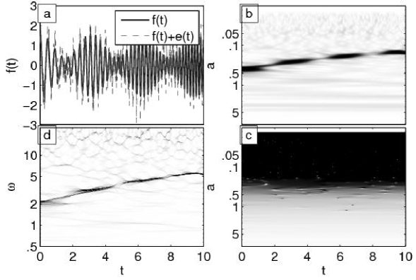
Figure 1: Synchrosqueezing example for $f(t)=(1+0.6\cos(2t))\cos(4\pi t+1.2t^{2})$ and additive noise $e(t)\sim{\mathcal{N}}(0,0.5^{2})$. Panels in clockwise order: a) $f(t)$ and $f(t)+e(t)$ sampled, $n=1024$ points. b) CWT of $f$, $|W_{f}|$. c) Phase transform ${\omega}_{f}$. d) Synchrosqueezing transform $|T_{f}|$; with $\gamma=10^{-5}$ (see §III-E).

III-A DWT of sampled signal: ${\widetilde{W}}_{{\tilde{f}}}$

We first choose an appropriate mother wavelet $\psi$. We pick $\psi$ such that its Fourier transform $\widehat{\psi}(\xi)$ (normalized as in Theorem II.1) is concentrated in absolute value around some positive frequency $\xi=\omega_{0}$, and is small and rapidly decaying elsewhere (i.e. $\lim_{|t|\to\infty}P(t)\psi(t)=0$ for all polynomials $P$). Many standard mother wavelets satisfy these properties, and we compare several examples in §IV-D.

The DWT samples the CWT $W_{f}$ at the locations $(a_{j},t_{m})$, where $a_{j}=2^{j/n_{v}}\Delta t$, $j=1,\ldots,Ln_{v}$, and the ”voice number” $n_{v}$ [22] is a user-defined parameter that affects the number of scales we work with (we have found that $n_{v}=32$ or $64$ works well in practice). The DWT of ${\tilde{f}}$ can be calculated in $O(n_{v}n\log_{2}^{2}n)$ operations using the FFT. We outline the steps below.

First note that $W_{f}(a,\cdot)=a^{-1/2}\overline{\psi(-\frac{\cdot}{a})}\star f$, where $\star$ denotes the convolution. In the frequency domain, this relationship becomes $\widehat{W}_{f}(a,\xi)=a^{1/2}\widehat{f}(\xi)\overline{\widehat{\psi}(a\xi)}$. We use this to calculate the DWT, ${\widetilde{W}}_{{\tilde{f}}}(a_{j},t_{m})$. Let ${\mathcal{F}}_{n}$ (${\mathcal{F}}_{n}^{-1}$) be the standard (inverse) circular Discrete Fourier Transform. Then

$${\widetilde{W}}_{{\tilde{f}}}(a_{j},\cdot)={\mathcal{F}}_{n}^{-1}\left(({\mathcal{F}}_{n}{\tilde{f}})\odot\overline{\widehat{\psi}_{j}}\right).$$ (12)

Here $\odot$ denotes elementwise multiplication and $\widehat{\psi}_{j}$ is an $n$-length vector with $(\widehat{\psi}_{j})_{m}=a_{j}^{1/2}\widehat{\psi}(a_{j}\xi_{m})$; $\xi_{m}$ are samples in the unit frequency interval: $\xi_{m}=2\pi m/n$, $m=0,\ldots,n-1$.

III-B The phase transform: $\widetilde{\omega}_{{\tilde{f}}}$

The next step is to calculate the phase transform (2). We first require a slight modification of the definition (2),

$$\omega_{f}(a,b)=\frac{1}{2\pi}\operatorname{\mathfrak{Im}}{\left((W_{f}(a,b))^{-1}\partial_{b}W_{f}(a,b)\right)}.$$ (13)

In theory Eqs. (13) and (2) are equivalent, and in practice (13) is a convenient way to obtain a real-valued frequency from (2). We denote the discretization of $\omega_{f}$ by $\widetilde{\omega}_{{\tilde{f}}}$.

In practice, signals have noise and other artifacts due to, e.g., sampling errors, and computing the phase of $W_{f}$ is unstable when $\left\lvert W_{f}\right\rvert\approx 0$. Therefore, we choose a hard threshold parameter $\gamma>0$ and disregard any points where $\left\lvert W_{f}\right\rvert\leq\gamma$ . The exact choice of $\gamma$ is discussed in Sec. III-E. We use this to define the numerical support of ${\widetilde{W}}_{{\tilde{f}}}$, on which $\omega_{f}$ can be estimated:

$\widetilde{{\mathcal{S}}}_{{\tilde{f}}}^{\gamma}(m)=\left\{j:\left\lvert{\widetilde{W}}_{{\tilde{f}}}(a_{j},t_{m})\right\rvert>\gamma\right\}$, for $m=0,\ldots,n-1$.

The derivative in (13) can be calculated by taking finite differences of ${\widetilde{W}}_{{\tilde{f}}}$ with respect to $m$, but Fourier transforms provide a more accurate alternative. Using the property $\widehat{\partial_{b}W_{f}}(a,\xi)=2\pi i\xi\widehat{W_{f}}(a,\xi)$, we estimate the phase transform, for $j\in\widetilde{{\mathcal{S}}}_{{\tilde{f}}}^{\gamma}(m)$, as

$\widetilde{\omega}_{{\tilde{f}}}(a_{j},t_{m})=\frac{1}{2\pi}\operatorname{\mathfrak{Im}}{\left(\left({\widetilde{W}}_{{\tilde{f}}}(a_{j},t_{m})\right)^{-1}\partial_{b}{\widetilde{W}}_{{\tilde{f}}}(a_{j},t_{m})\right)},$

with the derivative of $W_{f}$ estimated via (e.g., [43])

$\partial_{b}{\widetilde{W}}_{{\tilde{f}}}(a_{j},\cdot)={\mathcal{F}}_{n}^{-1}\left(({\mathcal{F}}_{n}{\tilde{f}})\odot\widehat{\partial\psi}_{j}\right),$

where $(\widehat{\partial\psi}_{j})_{m}=2\pi ia_{j}^{1/2}\xi_{m}\widehat{\psi}(a_{j}\xi_{m})/\Delta t$ for $m=0,\ldots,n-1$.

The normalization of $\widetilde{\omega}$ corresponds to a dominant, constant frequency of $\alpha$ when $f(t)=\cos(2\pi\alpha t)$. This allows us to transition from the time-scale plane to a time-frequency plane according to the reassignment map $(a,b)\to(\omega(a,b),b)$. Note that the phase transform is not the instantaneous frequency itself except in some simple cases, but contains requisite “frequency information” that we use to recover the actual frequencies in the next step.

III-C Synchrosqueezing in the time-frequency plane: ${T_{f}(\omega,b)}$

We now compute the Synchrosqueezing transform using the reassigned time-frequency plane. Suppose we have some “frequency divisions” $\left\{w_{l}\right\}_{l=0}^{\infty}$ with $w_{0}>0$ and $w_{l+1}>w_{l}$ for all $l$. Let the frequency bin ${\mathcal{W}}_{l}$ be given by $\{w^{\prime}\in{\mathbb{R}}:|w^{\prime}-w_{l}|<|w^{\prime}-w_{l^{\prime}}|\,\forall l^{\prime}\not=l\}$, or in other words, the set of points closer to $w_{l}$ than any other $w_{l^{\prime}}$. We define the discrete-frequency Wavelet Synchrosqueezing transform of $f$ by

$$T_{f}(w_{l},b)=\int_{\left\{a:\omega_{f}(a,b)\in{\mathcal{W}}_{l},|W_{f}(a,b)|>\gamma\right\}}W_{f}(a,b)a^{-3/2}da.$$ (14)

This is essentially the limiting case of the definition (3) as $\delta\to 0$ (note the argument in (9) and see also [14, p. 5-6]), but with the frequency variable $\eta\in{\mathbb{R}}$ replaced by the discrete intervals ${\mathcal{W}}_{l}$. Note that the discretization ${\widetilde{W}}_{{\tilde{f}}}$ is given with respect to $n_{a}=Ln_{v}$ log-scale samples of the scale $a$, so we correspondingly discretize (14) over a logarithmic scale in $a$. The transformation $a(z)=2^{z/n_{v}}$, $da(z)=a\frac{\log 2}{n_{v}}dz$, leads to the modified integrand ${W_{f}(a,b)a^{-1/2}\frac{\log 2}{n_{v}}dz}$ in (14).

To choose the frequency divisions $w_{l}$, note that the time step $\Delta t$ limits the range of frequencies that can be estimated. One form of the Nyquist sampling theorem shows that the maximum frequency is $\overline{w}=w_{n_{a}-1}=\frac{1}{2\Delta t}$. Since $f$ is discretized over an interval of length $n\Delta t$, the fundamental (minimum) frequency is $\underline{w}=w_{0}=\frac{1}{n\Delta t}$. Combining these bounds on a logarithmic scale, we get the divisions $w_{l}=2^{l\Delta w}\underline{w}$, $l=0,\ldots,n_{a}-1$, where $\Delta w=\frac{1}{n_{a}-1}\log_{2}(n/2)$.

We can now calculate a fully discretized estimate of (14), denoted by ${\widetilde{T}}_{{\tilde{f}}}$. Since we have already tabulated $\widetilde{\omega}_{{\tilde{f}}}$ and $\widetilde{\omega}_{{\tilde{f}}}(a_{j},t_{m})$ lands in at most one frequency bin ${\mathcal{W}}_{l}$, the integral in (14) can be computed efficiently by finding the associated ${\mathcal{W}}_{l}$ for each $(a_{j},t_{m})$ and adding it to the appropriate sum. This results in $O(n_{a}n)$ computations for the entire Synchrosqueezed plane ${\widetilde{T}}_{{\tilde{f}}}$. We summarize this approach in pseudocode in Alg. 1.

Algorithm 1 Fast calculation of ${\widetilde{T}}_{\tilde{f}}$ for fixed $m$

  for $l=0$ to $n_{a}-1$ do {Initialize ${\widetilde{T}}$ for this $m$}

     ${\widetilde{T}}_{{\tilde{f}}}(w_{l},t_{m})\leftarrow 0$

  end for

  for all $j\in\widetilde{{\mathcal{S}}}^{\gamma}_{{\tilde{f}}}(m)$ do {Calculate (14)}

     {Find frequency bin via $w_{l}=2^{l\Delta w}\underline{w}$, and $\widetilde{\omega}_{{\tilde{f}}}\in{\mathcal{W}}_{l}$}

     $l\leftarrow\min\left(\max\left(\textrm{ROUND}\left[\frac{1}{\Delta w}\log_{2}\left(\frac{\widetilde{\omega}_{{\tilde{f}}}(a_{j},b_{m})}{\underline{w}}\right)\right],0\right),n_{a}-1\right)$

     {Add normalized term to appropriate integral; $\Delta z=1$}

     ${\widetilde{T}}_{{\tilde{f}}}(w_{l},t_{m})\leftarrow{\widetilde{T}}_{{\tilde{f}}}(w_{l},t_{m})+\frac{\log 2}{n_{v}}{\widetilde{W}}_{{\tilde{f}}}(a_{j},t_{m})a^{-1/2}_{j}$

  end for

We remark that as an alternative, the frequency divisions $w_{l}$ can be spaced linearly, instead of the logarithmic scale we use in keeping with the discretization of the CWT in Section III-A. Examples of this approach can be found in [45], but in practice we find that there are no significant differences either way. In principle, the CWT itself can be discretized linearly as well, but the approach we took in Section III-A is standard and is preferred for its computational efficiency (see [13, 18]).

III-D Component reconstruction

We can finally recover each component $f_{k}$ from ${\widetilde{T}}_{{\tilde{f}}}$ by inverting the CWT (integrating) over the frequencies $w_{l}$ that correspond to the $k$th component, an approach similar to filtering on a conventional TF plot. Let $l\in\mathcal{L}_{k}(t_{m})$ be the indices of a small frequency band around the curve of $k$th component in the phase transform space (based on the results of Thm. II.2 and Thm. II.4 parts 2). These frequencies can be selected by hand or estimated via a standard least-squares ridge extraction method [9], as done in the Synchrosqueezing Toolbox. Then, using the fact that $f_{k}$ is real, we have

$$f_{k}(t_{m})=2{\mathcal{R}}_{\psi}^{-1}\operatorname{\mathfrak{Re}}{\left(\sum_{l\in\mathcal{L}_{k}(t_{m})}{\widetilde{T}}_{{\tilde{f}}}(w_{l},t_{m})\right)},$$ (15)

where ${\mathcal{R}}_{\psi}$ is the normalization constant from Theorem (II.1).

III-E Selecting the threshold $\gamma$

The hard wavelet threshold $\gamma$ effectively decides the lowest CWT magnitude at which $\omega$ is deemed trustworthy. In an ideal setting wherein the signal is not corrupted by noise, this threshold can be set based on the machine epsilon (we suggest $10^{-8}$ for double precision floating point systems). In practice, $\gamma$ can be seen as a hard threshold on the wavelet representation (shrinking small magnitude coefficients to $0$), and its value determines the level of filtering.

In [17], a nearly minimax optimal procedure was proposed for denoising sufficiently smooth signals corrupted by additive white noise. This algorithm consists of soft- or hard-thresholding the wavelet coefficients of the corrupted signal, followed by inversion of the filtered wavelet representation. In [16], this estimator was also shown to be nearly optimal in terms of root mean square error. The asymptotically optimal threshold is $\sqrt{2\log n}\cdot\sigma$, where $n$ is the signal length and $\sigma^{2}$ is the noise power. Following [17], the noise power can be estimated from the Median Absolute Deviation (MAD) of the finest level wavelet coefficients. This is the threshold we suggest and use throughout our simulations:

$$\gamma=1.4826\sqrt{2\log n}\cdot\text{MAD}(|{\widetilde{W}}_{{\tilde{f}}}|_{1:n_{v}})$$

where $1.4826$ is the multiplicative factor relating the MAD of a Gaussian distribution to its standard deviation, and $|{\widetilde{W}}_{{\tilde{f}}}|_{1:n_{v}}$ are the wavelet coefficient magnitudes at the $n_{v}$ finest scales (the first octave).

IV Numerical Simulations

In this section, we provide several numerical examples that illustrate the ideas in Sec. II and III and show how Synchrosqueezing compares to a variety of other time-frequency transforms in current use. The MATLAB scripts used to generate the figures for these examples are available at [8].

IV-A Comparison of Synchrosqueezing with the CWT, STFT and EEMD

We first compare the Synchrosqueezing time-frequency decomposition to the continuous wavelet transform (CWT) and the short-time Fourier transform (STFT) [34]. We show its superior precision, in both time and frequency, at identifying the components of complicated oscillatory signals. We then show its ability to reconstruct (via filtering) an individual component from a curve in the time-frequency plane. We also compare the recovered component with the results of the ensemble empirical mode decomposition (EEMD) method (see [46] for details).

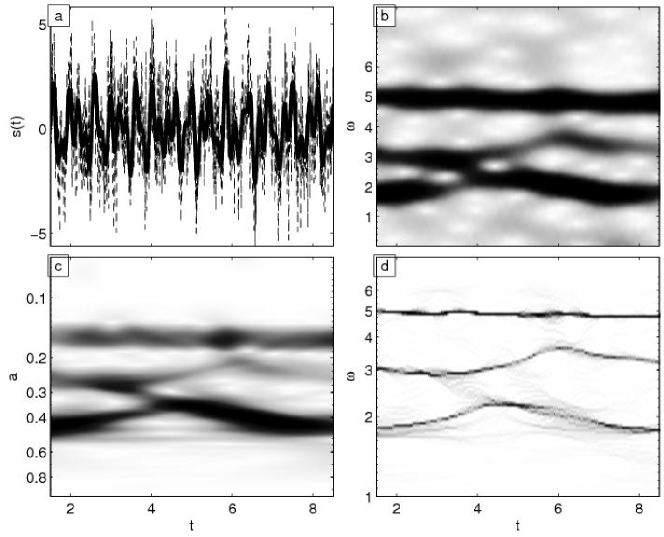
Figure 2: Comparison of Synchrosqueezing with the STFT and CWT. (a) Synthetic signal $s(t)$ (bold), corrupted with noise (dashed), shown for $t\in[2,8]$. (b) STFT of signal $s(t)$. (c) CWT of signal $s(t)$. (d) Synchrosqueezing plot $T_{s}(\omega,t)$.

In Fig. 2 we consider a signal $s(t)=s_{1}(t)+s_{2}(t)+s_{3}(t)+N(t)$ defined on $t\in[0,10]$ that contains different kinds of time-varying AM and FM modulation. It is composed of the following components:

$$s_{1}(t) =(1+0.2\cos(t))\cos(2\pi(2t+0.3\cos(t))),$$

$$s_{2}(t) =(1+0.3\cos(2t))e^{-t/15}\cos(2\pi(2.4t+0.5t^{1.2}+0.3\sin(t)))$$

$$s_{3}(t) =\cos(2\pi(5.3t+0.2t^{1.3})).$$

The signal is discretized to $n=2048$ points and corrupted by additive Gaussian white noise $N(t)$ with noise power $\sigma^{2}=2.4$, leading to an SNR of $-2.6$ dB.

To make the comparison consistent (as the $\gamma$ threshold in Synchrosqueezing has a denoising effect), we first denoise the signal using the Wavelet hard-thresholding methodology of §III-E. We then feed this denoised signal to the STFT, CWT, and Synchrosqueezing transforms. We use the shifted bump wavelet (see §IV-D) and $n_{v}=32$ for both the CWT and Synchrosqueezing transforms, and a Hamming window with length 400 and overlap of length 399 for the STFT. These STFT parameters are selected to have a representation visually balanced between time and frequency resolution [34].

The component $s_{3}$ is close to a Fourier harmonic and is clearly identified in the Synchrosqueezing plot $T_{s}$ (Fig. 2(d)) and the STFT plot (Fig. 2(b)), though the frequency estimate is more precise in $T_{s}$. The other two components have time-varying instantaneous frequencies and can be clearly distinguished in the Synchrosqueezing plot, while there is much more smearing and distortion in them in the STFT and CWT. The temporal resolution of the CWT and STFT is also significantly lower than for Synchrosqueezing due to the selected parameters. A shorter time window or wavelet will provide higher temporal resolution, but lower frequency resolution and more smearing between the three components.

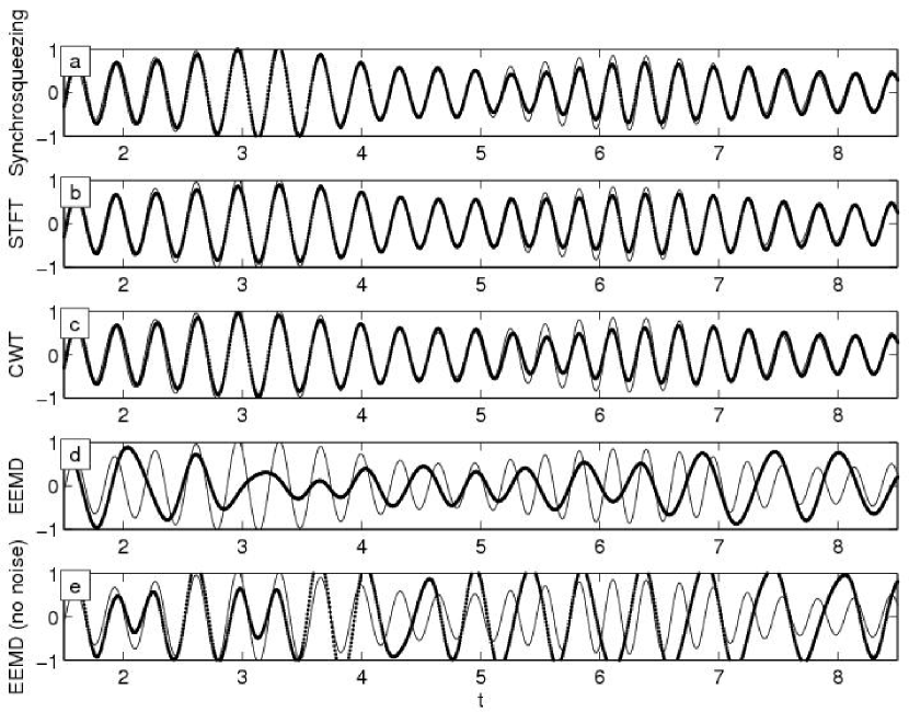
Figure 3: (a-c) Reconstruction of the component $s_{2}$ on $[2,8]$ performed by inverting Synchrosqueezing (a), CWT (b) and STFT (c), shown as dotted curves. (d-e) The EEMD extraction of $s_{2}$ with $50$ ensembles performed on the signal $s$ (d), and on the same signal without any noise and one ensemble (e). The original component $s_{2}$ is shown in solid curves for reference.

Fig. 3 shows the component $s_{2}$ reconstructed from the TF plots in Fig. 2 by inverting each transform in a small band around the curve of $s_{2}$. All three time-frequency methods provide comparable results and pick up the component reasonably accurately, although the AM behavior around $t\in[5,7]$ is slightly smothered out as a result of the noise. On the other hand, EEMD exhibits a poor amplitude recovery and a drifting phase over time, even when applied to the original signal without any noise. In general, EMD/EEMD is sensitive to amplitude changes over time that impose strong requirements on the frequency separation between the components [37], while Synchrosqueezing and the other time-frequency methods produce good results as long as the bandwidth of the mother wavelet or window is small enough, according to Theorem II.1.

IV-B Comparison of Synchrosqueezing with Reassignment Techniques

We next compare the analysis part of Synchrosqueezing to two of the most common time-frequency reassignment (TFR) methods, based on the spectrogram and the Wigner-Ville distribution (see [19], ch. 4 for details). We apply these techniques to $s(t)$, the signal from the last example, for $t\in[2,8]$ and with the noise increased to $\sigma^{2}=5$ ($-5.8$ dB SNR). The results are shown in Fig. 4.

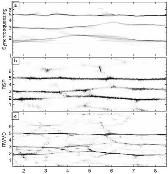
Figure 4: (a) Synchrosqueezing $\widetilde{T}_{{\tilde{f}}}$ of ${\tilde{f}}$. (b) Reassigned spectrogram / STFT of ${\tilde{f}}$ (RSP). (c) Reassigned smoothed pseudo-WVD of ${\tilde{f}}$ (RWVD).

Synchrosqueezing can be understood as a variant of the standard TFR methods. In TFR methods, the directional reassignment vector is computed in both time and frequency from the magnitude of the STFT or WVD, which is then used to remap the energies in the TF plane of a signal. In contrast, the Synchrosqueezing transform can be thought of as a reassignment vector only in the frequency direction. The fact that there are no time shifts in the TF plane is what allows the reconstruction of the signal to be possible. We note that in Fig. 4, the Synchrosqueezing TF plot contains fewer spurious components than the other TFR plots. The other TFR methods exhibit additional clutter in the TF plane caused by the noise, and the reassigned WVD also contains traces of an extra curve between the second and third components, a result of the quadratic cross-terms that are characteristic of the WVD [19].

IV-C Nonuniform Samples and Spline Fitting

We now demonstrate how Synchrosqueezing analysis and extraction works for a three-component signal that has been irregularly sampled. For $t\in[2,8]$, let

$$f(t) =(1+0.5\cos(t))\cos(4\pi t)$$ (16)

$$+2e^{-0.1t}\cos(2\pi(3t+0.25\sin(1.4t)))$$

$$+(1+0.5\cos(2.5t))\cos(2\pi(5t+2t^{1.3})),$$

and let the sampling times be perturbations of uniformly spaced times having the form $t^{\prime}_{m}=\Delta t_{1}m+\Delta t_{2}u_{m}$, where $\{u_{m}\}$ is sampled from the uniform distribution on $[0,1]$. We take $\Delta t_{1}=11/300$ and $\Delta t_{2}=11/310$, which leads to approximately $165$ samples on the interval $[2,8]$ and an average sampling rate of $27.2$, or about three times the maximum instantaneous frequency of $9.85$. As indicated in Cor. II.3, we account for the nonuniform sample spacing by fitting a cubic spline through $(t^{\prime}_{m},f(t^{\prime}_{m}))$ to get the interpolant $f_{s}(t)$, discretized on the finer grid $t_{m}=m\Delta t$ with $\Delta t=10/1024$ and $m=0,\ldots,1023$. The resulting vector, ${\tilde{f}}_{s}$, is a discretization of the original signal plus a spline error term $e(t)$.

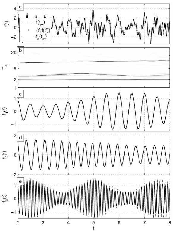
Figure 5: (a) Nonuniform samples of $f$, with spline interpolant ${\tilde{f}}_{s}$ (solid), and original signal $f$ (dashed). (b) Synchrosqueezing TF plane $\widetilde{T}_{{\tilde{f}}_{s}}$. (c-e) Extracted components ${\tilde{f}}^{*}_{k}$ for $k=1,2,3$ (solid) compared to originals ${\tilde{f}}_{k}$ (dashed).

Fig. 5(a-e) shows the Synchrosqueezing TF plot ${\tilde{f}}_{s}$ and the three reconstructed components. The spline interpolant approximates the original signal closely, except for a few oscillations for $t>7.3$ where the highest frequencies of $f$ occur. The Synchrosqueezing results are largely unaffected by the errors and have no spurious spectral information in the TF plot. The effect of the interpolation errors for $t>7.3$ is also localized in time and only influences the AM recovery of the third component, which contains the highest frequencies and is the most difficult to recover as indicated by Thm. II.2. In general, however, we find that components close to the Nyquist frequency are picked up fairly accurately as long as the mother wavelet is chosen according to Theorem II.1 and the components are spaced sufficiently far apart (for cases where multiple high frequency components are close together, see the STFT Synchrosqueezing approach in [44]).

IV-D Invariance to the underlying transform

As a final example, we show the effect of the underlying mother wavelet on the Synchrosqueezing transform. As discussed in [14], Synchrosqueezing is largely invariant to the choice of the mother wavelet, and the main differences one sees in practice are due to the wavelet’s relative concentrations in time and frequency (in particular, how far away its frequency content is from zero), as opposed to its precise shape.

Fig. 6 shows the effect of Synchrosqueezing on the discretized spline signal ${\tilde{f}}_{s}$ from the last example, using three different complex CWT mother wavelets. These wavelets are:

a. Morlet (shifted Gaussian)

$$\qquad\widehat{\psi}_{a}(\xi)\propto\exp(-2\pi^{2}(\mu-\xi)^{2}),\quad\xi\in{\mathbb{R}}$$

b. Complex Mexican Hat

$$\qquad\widehat{\psi}_{b}(\xi)\propto\xi^{2}\exp(-2\pi^{2}\sigma^{2}\xi^{2}),\quad\xi>0$$

c. Shifted Bump

$$\qquad\widehat{\psi}_{d}(\xi)\propto\exp\left(-(1-((2\pi\xi-\mu)/\sigma)^{2})^{-1}\right),$$

$$\qquad\xi\in[\sigma(\mu-1),\sigma(\mu+1)]$$

where for $\psi_{a}$ we use $\mu=1$, for $\psi_{b}$ we use $\sigma=1$, and for $\psi_{c}$ we use $\mu=5$ and $\sigma=1$. These respectively correspond to about $\Delta=0.5$, $0.25$ and $0.16$ in Thm. II.1. We find that, as indicated by Thm. II.1, the most accurate representation is given by the bump wavelet $\psi_{c}$, whose frequency support is the smallest and exactly (instead of approximately) positive and finite.

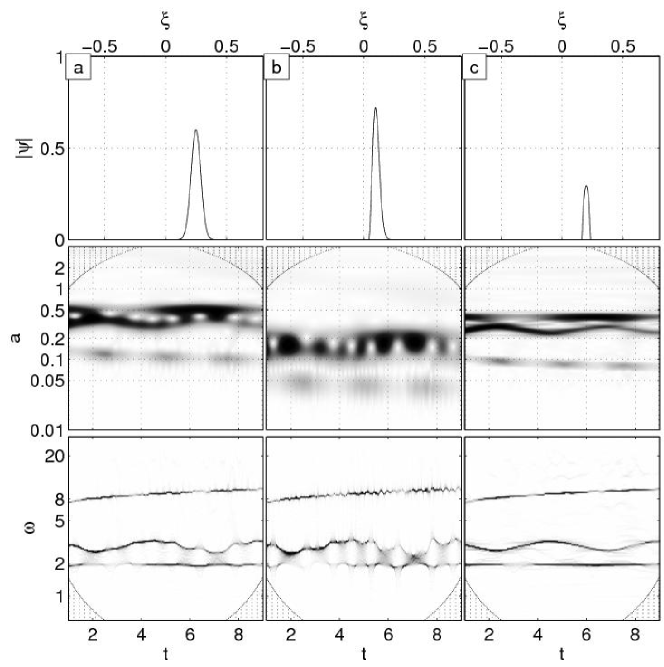
Figure 6: Wavelet and Synchrosqueezing transforms of ${\tilde{f}}_{s}$. Columns (a-c) represent choice of mother wavelet $\psi_{a}\ldots\psi_{c}$. Top row: $|2\widehat{\psi}(4\xi)|$. Center row: $|W_{f_{s}}|$. Bottom row: $|T_{f_{s}}|$.

V Aspects of the mid-Pleistocene transition

In this section, we apply Synchrosqueezing to analyze the characteristics of a calculated index of the incoming solar radiation (insolation) and paleoclimate records of repeated transitions between glacial (cold) and interglacial (warm) climates, i.e., ice age cycles, primarily during the Pleistocene epoch (from $\approx$ 1.8 Myr to $\approx$ 12 kyr before the present). The analysis of time series is crucial for paleoclimate research becuase its empirical base consists of a growing collection of long deposited records.

The Earth’s climate is a complex, multi-component, nonlinear system with significant stochastic elements [35]. The key external forcing field is the insolation at the top of the atmosphere (TOA). Local insolation has predominantly harmonic characteristics in time (diurnal cycle, annual cycle and very long Milanković orbital cycles) enriched by the solar variability. The response of the planetary climate, which varies at all time scales [26], also depends on random perturbations (e.g., volcanism), nonstationary solid boundary conditions (e.g., plate tectonics and global ice distribution), internal variability and feedback (e.g., global carbon cycle). Various paleoclimate records, called proxies, provide us with information about past climates beyond observational records. These proxies are biogeochemical tracers, i.e. molecular or isotopic properties, imprinted into various types of deposits (e.g., deep-sea sediment, ice cores, etc.), and they indirectly represent physical conditions (e.g. temperature) at the time of deposition. We focus on climate variability during the last 2.5 Myr (that also includes the late Pliocene and the Holocene) as recorded by ${\delta}^{18}O$ The oxygen isotope variations in seawater are expressed as deviations of the ratio of ${}^{18}O$ to ${}^{16}O$ with respect to the present-day standard. Carbonate shells of foraminifera plankton (benthic forams) at the bottom of the ocean record ${\delta}^{18}O$ changes in seawater during their growth. The benthic ${\delta}^{18}O$ indicates changes in the global sea level, ice volume and deep ocean temperature. During the buildup of land ice sheets and the decrease in sea level in cold climates, the lighter ${}^{16}O$ evaporates more readily than ${}^{18}O$ and accumulates in ice sheets, leaving the surface water enriched with ${}^{18}O$. At the same time, the inclusion of ${}^{18}O$ during the formation of carbonate shells records the ambient seawater temperature of the benthic forams [29].

Figure 7: (a) Calculated June 21 TOA insolation flux at $65^{o}N$: $f_{SF}$. Climate response as recorded by benthic forams ${\delta}^{18}O$ (b) in the DSDP607 core $f_{CR1}$, (c) in the LR05 stack $f_{CR2}$, and (d) in the H07 stack $f_{CR3}$.

We first examine a calculated element of the daily TOA solar forcing field. Fig. 7(a) shows $f_{SF}$, the mid-June insolation at $65^{o}N$ at 1 kyr intervals [5]. This TOA forcing index has been widely used to gain insight into the timing of advances and retreats of ice sheets in the Northern Hemisphere during this period, based on the classic Milanković hypothesis that summer solstice insolation at $65^{o}N$ paces ice age cycles (e.g., [23, 4]). The CWT and Synchrosqueezing spectral decompositions (using the shifted bump mother wavelet as in the rest of the paper), in Fig. 8(a) and Fig. 8(e) respectively, show the key time-varying oscillatory components of $f_{SF}$. Both panels confirm the presence of strong precession cycles (at periodicities $\tau$=19 kyr and 23 kyr), obliquity cycles (primary at 41 kyr and secondary at 54 kyr), and very weak eccentricity cycles (primary periodicities at 95 kyr and 124 kyr, and secondary at 400 kyr). However, the Synchrosqueezing spectral structure is far more concentrated along the frequency (periodicity) direction than the CWT.

We next analyze the North Altantic and global climate response during the last 2.5 Myr as deposited in benthic ${\delta}^{18}O$ in long sediments cores (in which deeper layers contain forams settled further back in time). Fig. 7(b) shows $f_{CR1}$: benthic ${\delta}^{18}O$, sampled at irregular time intervals from a single core, DSDP Site 607, in the North Atlantic [40]. Fig. 7(c) shows $f_{CR2}$: the orbitally tuned benthic ${\delta}^{18}O$ stack of [32] (LR05). It is an average of 57 globally distributed records placed on a common age model using a graphic correlation technique [31]. Fig. 7(d) shows $f_{CR3}$: the benthic ${\delta}^{18}O$ stack of [25] (H07) calculated from 14 cores (mostly in the Northern Hemisphere) using the extended depth-derived age model free from orbital tuning [27]. The ${\delta}^{18}O$ records included in these stacks vary over different ranges primarily due to different ambient temperatures at different depths of the ocean floor at core drill sites. Also, prior to combining the cores in the H07 stack, the record mean between 0.7 Myr ago and the present was subtracted from each ${\delta}^{18}O$ record, so we have different vertical ranges in Fig. 7(b) through Fig. 7(d). All ${\delta}^{18}O$ records are spline interpolated to 1 kyr intervals prior to the spectral analysis.

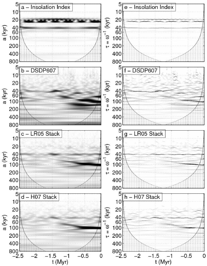
Figure 8: The CWT time-scale decomposition of (a) the solar forcing index $f_{SF}$, and the climate response in benthic ${\delta}^{18}O$ of (b) the DSDP607 core $f_{CR1}$, (c) the LR05 stack $f_{CR2}$, and (d) the H07 stack $f_{CR3}$. The Synchrosqueezing time-periodicity decomposition of (e) the solar forcing index $f_{SF}$, and the climate response in benthic ${\delta}^{18}O$ of (f) the DSDP607 core $f_{CR1}$, (g) the LR05 stack $f_{CR2}$, and (h) the H07 stack $f_{CR3}$.

The Synchrosqueezing decomposition in the right panels in Fig. 8 is a far more precise time-frequency representation of signals from DSDP607 and the stacks than the CWT decomposition in left panels in Fig. 8 or an STFT analysis of the H07 stack [25, Fig. 4]. Noise due to local characteristics and measurement errors of each core is reduced when we shift the spectral analysis from DSDP607 to the stacks, and this is particularly visible in the finer scales and higher frequencies. In addition, the stacks in Fig. 8(g) and Fig. 8(h) show far less stochasticity above the obliquity band (higher frequencies) compared to DSDP607 in Fig. 8(f). This enables the 23 kyr precession cycle to appear mostly coherent over the last 1 Myr, especially in comparison to the CWT decompositions. Thanks to the stability of Synchrosqueezing, the spectral differences below the obliquity band (lower frequencies) are less pronounced betweeen the stacks and DSDP607. Overall, the stacks show less noisy time-periodicity evolution than DSDP607 or any other single core due to the averaging of multiple, noisy time series with shared signals. The Synchrosqueezing decompositions are much sharper than the corresponding CWT decompositions, and a time average of the Synchrosqueezing magnitudes delineates the harmonic components more clearly than a comparable Fourier spectrum (not shown).

During the last 2.5 Myr, the Earth experienced a gradual decrease in the global long-term temperature and $\text{CO}_{2}$ concentration, and an increase in mean global ice volume accompanied with glacial-interglacial oscillations that have intensified towards the present (shown in Fig. 7(b) through Fig. 7(d)). The mid-Pleistocene transition, occurring abruptly or gradually sometime between 1.2 Myr and 0.6 Myr ago, was marked by the the shift from 41 kyr-dominated glacial cycles to 100 kyr-dominated glacial cycles recorded in deep-sea proxies (e.g., [39, 33, 12]). The cause of the emergence of strong 100 kyr cycle in the late-Pleistocene climate and incoherency of the precession band prior to about 1 Myr (evident in Fig. 8(g) and Fig. 8(h)) are still unresolved questions. Both types of spectral analyses of selected ${\delta}^{18}O$ records indicate that the climate system does not respond linearly to external solar forcing.

The Synchrosqueezing decomposition precisely reveals key modulated signals that rise above the stochastic background. The gain (the ratio of the climate response amplitude to insolation forcing amplitude) at a given frequency or period, is not constant due to the nonlinearity of the climate system. The 41 kyr obliquity cycle of the global climate response is present almost throughout the entire Pleistocene in Fig. 8(g) and Fig. 8(h). The most prominent feature of the mid-Plesitocene transition is the initiation of a lower frequency signal ($\approx$ 70 kyr) about 1.2 Myr ago that gradually evolves into the dominant 100 kyr component in the late Pleistocene (starting about 0.6 Myr ago). Finding the exact cause for this transition in the dominant ice age periodicity is beyond the scope of our paper, but the Synchrosqueezing analysis of the stacks shows that it is not a direct cause-and-effect response to eccentricity variability (very minor variation of the total insolation).

The precision of the Synchrosqueezing decomposition allows us to achieve a more accurate inversion across any limited frequency band of interest than the CWT spectrum. Inverting the Synchrosqueezing transform over the key orbital periodicity bands (i.e. filtering) in Fig. 9 emphasizes the nonlinear relationship between the TOA insolation and climate evolution. The top panels in Fig. 9, left to right, show rapidly diminishing contributions to the insolation from precession to eccentricity. However, all of the panels below the top row in Fig. 9 show a moderately increasing amplitude of variability, i.e., the inverse cascade of climate response with respect to $f_{SF}$ from the precession to the eccentricity band in the late-Pleistocene (after $\approx$ 0.6 Myr). On average, the obliquity band contains more power than the precession band in DSDP607 and both stacks. Internal feedback mechanisms, most likely due to the long-term cooling of the global climate, amplify the response of the eccentricity band after the early-Pleistocence (after $\approx$ 1.2 Myr). The cross-band differences in Fig. 9 (rows 2-4) indicate that a superposition of precession cycles can modulate the climate response in lower frequency bands, particularly in the eccentricity band, as the climate drifts into a progressively colder and potentially more nonlinear state (e.g., [6, 36]).

The Synchrosqueezing analysis of the solar insolation index and benthic $\delta^{18}O$ records makes a new contribution in three important ways. First, it produces sharper spectral traces of a complex system’s evolution through the high-dimensional climate state space than the CWT (e.g., [7, Fig. 2]) or STFT (e.g., [12, Fig. 2]). Second, it better delineates the effects of noise on specific frequency ranges when comparing a single core to a stack. Low frequency components are mostly robust to noise induced by local climate variability, deposition processes and measurement techniques. Third, Synchrosqueezing allows for a more accurate reconstruction of the signal components within frequency bands of interest than the CWT or STFT. Questions about the key processes governing large-scale climate variability over the last 2.5 Myr can be answered by using high-precision data analysis methods such as Synchrosqueezing, in combination with a hierarchy of dynamical models at various levels of complexity that reproduce the key aspects of the Pliocene-Pleistocene history. The resulting understanding of past climate epochs may benefit predictions of the future climate. [41]

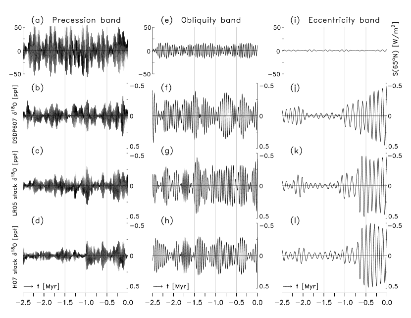
Figure 9: Milanković orbital components extracted by inverting the Synchrosqueezing transforms of the insolation index $f_{SF}$ (a, e, and i), and the climate response in benthic ${\delta}^{18}O$ from the DSDP607 core $f_{CR1}$ (b, f, and j), the LR05 stack $f_{CR2}$ (c, g, and k) and the H07 stack $f_{CR3}$ (d, h, and l). The transforms are inverted over the precession band from 17 kyr to 25 kyr (left column), the obliquity band from 40 kyr to 55 kyr (middle column), and the eccentricity band from 90 kyr to 130 kyr (right column).

VI Conclusions and Future Directions

Synchrosqueezing can be used to spectrally analyze and decompose a wide variety of signals with high precision in time and frequency. An efficient implementation runs in $O(n_{v}n\log^{2}n)$ time and is stable against errors in the signals, both in theory and in practice. We have shown how it can be used to gain further insight into the climate evolution of the past 2.5 million years.

The authors are also using the Synchrosqueezing transform to study additional topics in climate dynamics, meteorology and oceanography (climate variability and change, and large-scale teleconnection), as well as topics in ECG analysis (respiration and T-end detection, [10]). Synchrosqueezing is also being used by others to address problems in the analysis of mechanical transmissions [30] and the design of automated trading systems [1].

References

• [1] A. Ahrabian, C. C. Took, and D. Mandic. Algorithmic Trading Using Phase Synchronization. IEEE Journal of Selected Topics in Signal Processing, 99, 2012.
• [2] J.B. Allen and L.R. Rabiner. A unified approach to short-time fourier analysis and synthesis. Proceedings of the IEEE, 65(11):1558–1564, 1977.
• [3] F. Auger and P. Flandrin. Improving the readability of time-frequency and time-scale representations by the reassignment method. IEEE Transactions on Signal Processing, 43(5):1068 –1089, may 1995.
• [4] A. Berger. Milankovitch theory and climate. Review of Geophysics, 26(4):624–657, 1988.
• [5] A. Berger and M.F. Loutre. Insolation values for the climate of the last 10 million years. Quaternary Science Reviews, 10(4):297–317, 1991.
• [6] A. L. Berger. Support for the astronomical theory of climatic change. Nature, 269:44–45, 1977.
• [7] E. W. Bolton, K. A. Maasch, and J. M. Lilly. A wavelet analysis of Plio-Pleistocene climate indicators: A new view of periodicity evolution. Geophys. Res. Lett., 22(20):2753–2756, 1995.
• [8] E. Brevdo and H.-T. Wu. The Synchrosqueezing Toolbox. 2011. https://web.math.princeton.edu/~ebrevdo/synsq/.
• [9] R. A. Carmona, W. L. Hwang, and B. Torresani. Characterization of Signals by the Ridges of Their Wavelet Transforms. IEEE Transactions on Signal Processing, 45(10):2586–2590, 1997.
• [10] Y.-H. Chan, H.-T. Wu, S.-S. Hseu, C.-T. Kuo, and Y.-H. Yeh. ECG-Derived Respiration and Instantaneous Frequency based on the Synchrosqueezing Transform: Application to Patients with Atrial Fibrillation. arXiv preprint 1105.1571, 2011. http://arxiv.org/abs/1105.1571.
• [11] T. Claasen and W.F.G. Mecklenbrauker. The Wigner distribution: a tool for time frequency signal analysis. Philips J. Res, 35(3):217–250, 1980.
• [12] P.U. Clark, D. Archer, D. Pollard, J.D. Blum, J.A. Rial, V. Brovkin, A.C. Mix, N.G. Pisias, and M. Roy. The middle Pleistocene transition: characteristics, mechanisms, and implications for long-term changes in atmospheric pCO2. Quaternary Science Reviews, 25(23-24):3150–3184, 2006.
• [13] I. Daubechies. Ten Lectures on Wavelets. CBMS-NSF Regional Conference Series. SIAM, Philadelphia, PA, 1992.
• [14] I. Daubechies, J. Lu, and H.-T. Wu. Synchrosqueezed wavelet transforms: An empirical mode decomposition-like tool. Applied and Computational Harmonic Analysis, 30(2):243–261, 2011.
• [15] I. Daubechies and S. Maes. A nonlinear squeezing of the continuous wavelet transform based on auditory nerve models. Wavelets in Medicine and Biology, pages 527–546, 1996.
• [16] D.L. Donoho. De-noising by soft-thresholding. Information Theory, IEEE Transactions on, 41(3):613–627, 1995.
• [17] D.L. Donoho and J.M. Johnstone. Ideal spatial adaptation by wavelet shrinkage. Biometrika, 81(3):425, 1994.
• [18] D. L. Donoho et al. Wavelab. http://www-stat.stanford.edu/ wavelab.
• [19] P. Flandrin. Time-frequency/time-scale analysis, volume 10 of Wavelet Analysis and its Applications. Academic Press Inc., San Diego, CA, 1999.
• [20] S.A. Fulop and K. Fitz. Algorithms for computing the time-corrected instantaneous frequency (reassigned) spectrogram, with applications. J. Acoust. Soc. Am., 119:360, 2006.
• [21] R. Gallager. Circularly-Symmetric Gaussian random vectors. January 2008. http://www.rle.mit.edu/rgallager/documents/CircSymGauss.pdf.
• [22] P. Goupillaud, A. Grossmann, and J. Morlet. Cycle-octave and related transforms in seismic signal analysis. Geoexploration, 23(1):85–102, 1984.
• [23] J.D. Hays, J. Imbrie, NJ Shackleton, et al. Variations in the Earth’s orbit: pacemaker of the ice ages. Science, 194(4270):1121–1132, 1976.
• [24] N.E. Huang, Z. Shen, S.R. Long, M.C. Wu, H.H. Shih, Q. Zheng, N.C. Yen, C.C. Tung, and H.H. Liu. The empirical mode decomposition and the Hilbert spectrum for nonlinear and non-stationary time series analysis. Proceedings: Mathematical, Physical and Engineering Sciences, 454(1971):903–995, 1998.
• [25] P. Huybers. Glacial variability over the last two million years: an extended depth-derived agemodel, continuous obliquity pacing, and the Pleistocene progression. Quaternary Science Reviews, 26(1-2):37–55, 2007.
• [26] P. Huybers and W. Curry. Links between annual, Milankovitch and continuum temperature variability. Nature, 441(7091):329–332, 2006.
• [27] P. Huybers and C. Wunsch. A depth-derived Pleistocene age model: Uncertainty estimates, sedimentation variability, and nonlinear climate change. Paleoceanography, 19, 2004.
• [28] H-H. Kuo. White Noise Distribution Theory. CRC Press, 1996.
• [29] D.W. Lea. Elemental and Isotopic Proxies of Marine Temperatures. In The Oceans and Marine Geochemistry (ed. H. Elderfield), pages 365–390. Elsevier-Pergamon, Oxford.
• [30] C. Li and M. Liang. Time-frequency analysis for gearbox fault diagnosis using a generalized synchrosqueezing transform. Mechanical Systems and Signal Processing, 26:205–217, 2012.
• [31] L. E. Lisiecki and P. A. Lisiecki. Application of dynamic programming to the correlation of paleoclimate records. Paleoceanography, 17(D4), 2002.
• [32] L. E. Lisiecki and M. E. Raymo. A Pliocene-Pleistocene stack of 57 globally distributed benthic d18O records. Paleoceanography, 20, 2005.
• [33] M. Mudelsee and M. Schulz. The Mid-Pleistocene climate transition: onset of 100 ka cycle lags ice volume build up by 280 ka. Earth and Planetary Science Letters, 151:117–123, 1997.
• [34] A.V. Oppenheim, R.W. Schafer, and J.R. Buck. Discrete-Time Signal Processing. Prentice Hall, 1999.
• [35] R.T. Pierrehumbert. Principles of planetary climate. Cambridge University Press, 2010.
• [36] A.J. Ridgwell, A.J. Watson, and M.E. Raymo. Is the spectral signature of the 100 kyr glacial cycle consistent with a Milankovitch origin? Paleoceanography, 14(4):437–440, 1999.
• [37] G. Rilling and P. Flandrin. One or Two Frequencies? The Empirical Mode Decomposition Answers. IEEE Transactions on Signal Processing, 56:85–95, January 2008.
• [38] O. Rioul and P. Flandrin. Time-scale energy distributions: A general class extending wavelet transforms. Signal Processing, IEEE Transactions on, 40(7):1746–1757, 1992.
• [39] W.F. Ruddiman, M. Raymo, and A. McIntyre. Matuyama 41,000-year cycles: North Atlantic Ocean and northern hemisphere ice sheets. Earth and Planetary Science Letters, 80(1-2):117–129, 1986.
• [40] W.F. Ruddiman, M.E. Raymo, D.G. Martinson, B.M. Clement, and J. Backman. Pleistocene evolution: northern hemisphere ice sheets and North Atlantic Ocean. Paleoceanography, 4(4):353–412, 1989.
• [41] L Skinner. Facing future climate change: is the past relevant? Philosophical Transactions of the Royal Society A: Mathematical, Physical and Engineering Sciences, 366(1885):4627–4645, 2008.
• [42] G.W. Stewart. Afternotes goes to graduate school: lectures on advanced numerical analysis. Society for Industrial Mathematics, 1998.
• [43] E. Tadmor. The exponential accuracy of Fourier and Chebyshev differencing methods. SIAM Journal on Numerical Analysis, 23(1):1–10, 1986.
• [44] G. Thakur and H.-T. Wu. Synchrosqueezing-based Recovery of Instantaneous Frequency from Nonuniform Samples. SIAM Journal on Mathematical Analysis, 43(5):2078–2095, 2011.
• [45] H.-T. Wu. Instantaneous frequency and wave shape functions (i). Applied and Computational Harmonic Analysis, 2012.
• [46] Z. Wu and N.E. Huang. Ensemble empirical mode decomposition: a noise-assisted data analysis method. Advances in Adaptive Data Analysis, 2008.