SLAC-PUB-14373 Reducing Memory Cost of Exact Diagonalization using Singular Value Decomposition

Abstract

We present a modified Lanczos algorithm to diagonalize lattice Hamiltonians with dramatically reduced memory requirements, without restricting to variational ansatzes. The lattice of size $N$ is partitioned into two subclusters. At each iteration the Lanczos vector is projected into two sets of $n_{{\rm svd}}$ smaller subcluster vectors using singular value decomposition. For low entanglement entropy $S_{ee}$, (satisfied by short range Hamiltonians), the truncation error is expected to vanish as $\exp(-n_{{\rm svd}}^{1/S_{ee}})$. Convergence is tested for the Heisenberg model on Kagomé clusters of 24, 30 and 36 sites, with no lattice symmetries exploited, using less than 15GB of dynamical memory. Generalization of the Lanczos-SVD algorithm to multiple partitioning is discussed, and comparisons to other techniques are given.

I Introduction

Numerical (”exact”) diagonalizations (ED) of quantum many-body Hamiltonians on finite clusters are often used to advance our understanding of larger lattices. For example, Contractor Renormalization CORE-W ; CORE-A ; CORE-S uses ED to compute the short range interactions of the effective hamiltonian. ED on various size clusters LauchliED are indispensable as unbiased tests of mean field theories and variational wavefunctions. They are also used to obtain short wavelength dynamical correlations SXX and Chern numbers of Hall conductivity Chern .

ED commonly use Lanczos algorithms Lanczos-original ; cullum , to efficiently converge to the low eigenstates. However, for a lattice of size $N$, with $m$ states per site, the dimension of the Lanczos vectors (which are stored in the dynamical memory) increases as $m^{N}$. Therefore, ED on larger lattices are prevented primarily by memory limitations, rather than processor speed.

The central idea of this paper is to significantly reduce the memory cost, in order to enable ED of larger lattice sizes. We use singular value decomposition (SVD) to compress all Lanczos vectors into sets of $2n_{\rm{svd}}$ vectors of size $m^{N/2}$.

As long as entanglement entropy of the target eigenstates obeys $S_{ee}<<N/2\log(m)$ entanglementRMP , one can greatly economize on memory while maintaining high numerical accuracy. Many of the important many body Hamiltonians of condensed matter (e.g. Hubbard and Heisenberg models) have short range interactions. As a consequence, their ground states possess low entanglement entropy EE1 ; EE2 ; EE3 ; EE4 .

The idea of exploiting low entanglement entropy to compress wavefunctions by SVD, is not new. This is the key to the remarkable success of density matrix renormalization group (DMRG) whitedmrg which has been used extensively to obtain low energy state correlations of a large variety of Hamiltonians. DMRG is equivalent to variational minimization in the space of matrix product states Ostlund ; EE1 ; PPB . Extensions to wavefunctions with longer range correlations were given by multiscale entanglement renormalization mera-prl . Nevertheless, sequential minimization may sometimes get ”stuck” in false minima and not converge to the ground state. Therefore Lanczos methods are often called for to independently test the variational results.

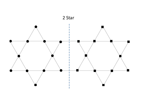
Figure 1: Partitioning 24 sites Kagomé cluster for application of the Lanczos-SVD algorithm. The ground state entanglement entropy is $S_{ee}=1.51$.

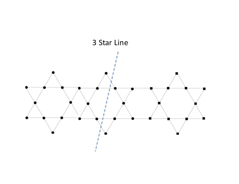
Figure 2: Partitioning 36 sites for three stars in a line. Ground state entanglement entropy is $S_{ee}\approx 1.12$.

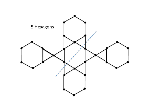
Figure 3: Partitioning of 30 sites containing 5 hexagons. Ground state entanglement entropy is $S_{ee}\approx 1.27$.

Figure 4: Partitioning 36 sites. Ground state entanglement entropy is $S_{ee}\approx 2.59$.

The paper is organized as follows. We begin by defining the SVD for a bipartite split of the lattice, and proceed to explain in practice how perform a single Lanczos step followed by an SVD projection which prevents the expansion of the memory cost. We describe the intermediate matrix manipulations needed for orthonormalizations and diagonalizations. In Section III, we estimate the SVD truncation error after projection, as a function of $n_{{\rm svd}}$. We relate the error estimation to the bipartite entanglement entropy $S_{ee}$, using a generic asymptotic form for the entanglement spectrum which is based on a classical gas model. We test in detail, the convergence of the Lanczos-SVD algorithm for the spin half Heisenberg antiferromagnet on Kagomé clusters of up to 36 sites. The entanglement spectrum asymptotics are verified for a partitioning of a 30 site cluster, Fig. 3. The ground state energy of 36 sites with Lanczos-SVD converges to relative errors of $6\times 10^{-8}$ for the three star line, Fig. 2, and $1.3\times 10^{-4}$ for the three star triangle, Fig. 4. Here we use a desktop computer with less than 15GB of memory and no lattice symmetries. The results agree with our analytical estimate of the truncation error. In Section VI we discuss a possible extension of this approach to multi-partitioning, and estimate the optimal reduction in memory cost that could be achieved. We conclude by a discussion which elaborates on the relative advantages and disadvantages of Lanczos-SVD, standard Lanczos and DMRG.

II The Lanczos-SVD Step

II.1 Bipartite Singular Value Decomposition

Any state $|\psi\rangle$ of the full cluster (see as an example Fig. 1) can be represented in a unique SVD form as

$$|\psi\rangle = \sum_{\alpha}\lambda_{\alpha}|\alpha\rangle_{1}|\alpha\rangle_{2},$$

$$\sum_{\alpha}\lambda_{\alpha}^{2} = 1,~{}~{}~{}~{}\langle\alpha|\alpha^{\prime}\rangle_{i}=\delta_{\alpha\alpha^{\prime}},$$ (1)

where the $\lambda_{\alpha}$ are positive, and $|\alpha\rangle_{i}$ are ”small” basis vectors of subclusters $i=1,2$ (the subclusters on the two sides of the partitioning). Truncating the sum into the largest $n_{{\rm svd}}$ terms defines the SVD projector,

$$P_{{\rm svd}}|\psi\rangle=\sum_{\alpha=1}^{n_{{\rm svd}}}\lambda_{\alpha}|\alpha\rangle_{1}|\alpha\rangle_{2},$$ (2)

which introduces a wavefunction error $\epsilon=\sum_{\alpha>n_{{\rm svd}}}\lambda_{\alpha}^{2}$.

II.2 Application of $P_{{\rm svd}}H$

Lanczos-SVD economizes on the storage space by applying an SVD projection after each application of the Hamiltonian on the Lanczos vector,

$$|\psi\rangle^{\prime}=P_{{\rm svd}}H|\psi\rangle.$$ (3)

The projection entails the following computational steps. $H$ can be written as a sum of products of the two subcluster operators,

$$H=H^{0}_{1}\otimes I_{2}+I_{1}\otimes H^{0}_{2}+\sum_{\mu=3}^{M}H_{1}^{\mu}\otimes H_{2}^{\mu}.$$ (4)

where $H^{0}_{i}$ includes all internal interactions of subcluster $i$. $H_{1}^{\mu}\otimes H_{2}^{\mu}$ is a product of operators residing on both subclusters. For example, a nearest neighbor Heisenberg model ($\sum_{ij}{\bf S}_{i}\cdot{\bf S}_{j}$) with $K$ bonds connecting the two subclusters has $M=2+3K$ terms. For example in Fig. 4, $K=7$ and $M=23$.

Acting with $H$ on $|\psi\rangle$ produces a new state,

$${H}|\psi\rangle=\sum_{\nu=1}^{n_{\rm{svd}}M}|\nu)_{1}|\nu)_{2},$$ (5)

where the new (non orthonormal) small vectors are labeled by the fused index $\nu=(\mu,\alpha)~{}$, i.e. $|\nu)_{i}=H^{\mu}_{i}|\alpha\rangle_{i}$. The state (5) lies outside the $n_{{\rm svd}}$ subspace, and we need to project it back using $P_{{\rm svd}}$ in order not to further expand the memory cost. We first orthonormalize $|\nu)_{i}$ by diagonalizing the Hermitian overlap matrices (of row dimensions $n_{\rm{svd}}M$)

$$\langle\nu^{\prime}|\nu\rangle_{i} = \left(V_{i}^{\dagger}D_{i}V_{i}\right)_{\nu\nu^{\prime}}~{}~{}~{}~{}i=1,2$$

$$|\beta\rangle_{i} = \sum_{\nu}\left(D_{i}^{-\mbox{$1\over 2$}}V_{i}\right)_{\beta\nu}|\nu)_{i},$$ (6)

where $D_{i}$ are diagonal and positive semidefinite, and $V_{i}$ are unitary. $|\beta\rangle_{i},i=1,2$ are orthonormal sets in their respective spaces. Thus, the new vector is given by

$$H|\psi\rangle = \sum_{\beta\beta^{\prime}}^{n_{\beta}n_{\beta^{\prime}}}C_{{\beta}{\beta^{\prime}}}|\beta\rangle_{1}|\beta^{\prime}\rangle_{2}$$

$$C = \sqrt{D_{1}}V_{1}^{*}V_{2}^{\dagger}\sqrt{D_{2}}.$$ (7)

Now we perform an SVD on the matrix $C$,

$$C=\nu_{c}^{2}U_{1}^{t}\Lambda^{\prime}U_{2},$$ (8)

where $\nu_{c}$ is the normalization. $U_{1}^{t},U_{2}^{\dagger}$ are unitary matrices which diagonalize the Hermitian products $CC^{\dagger}$ and $C^{\dagger}C$ respectively. After computing $\Lambda,U_{1},U_{2}$ we obtain the SVD form of the new state. $\Lambda$ is diagonal and normalized to $\mbox{Tr}\Lambda^{2}=1$ with positive eigenvalues $\lambda_{\alpha}^{\prime}$. We keep only the $n_{{\rm svd}}$ largest $\lambda_{\alpha}^{\prime}$ and obtain

$$P_{{\rm svd}}H|\psi\rangle=\sum_{\alpha=1}^{n_{\rm{svd}}}\lambda^{\prime}_{\alpha}|\alpha\rangle_{1}^{\prime}|\alpha\rangle_{2}^{\prime},$$ (9)

where the new small vectors of $i=1,2$ are,

$$|\alpha\rangle_{i}^{\prime}=\sum_{\nu=1}^{n_{\rm{svd}}M}\left(U_{i}D^{-{1\over 2}}V_{i}\right)_{\alpha\nu}|\nu)_{i}.$$ (10)

III Entanglement spectrum and SVD truncation error

The Lanczos algorithm rotates a set of basis states $|\psi_{n}\rangle$ into the lowest energy eigenstates with which the basis has a finite overlap. If we choose $\epsilon$ to be much smaller than the lowest relative energy gap, the Lanczos-SVD vectors converge to a states which are within $\epsilon$ distance from the SVD projection of the corresponding exact eigenstate.

To get an idea of how $\epsilon(n_{{\rm svd}})$ converges, we must know the ”entanglement spectrum” $\{s_{\alpha}\}$ defined by $\lambda^{2}_{\alpha}\equiv e^{-s_{\alpha}}$. $s_{\alpha}$ are pseudo-energies of the entanglement spectrum. A generic density of states can be modeled by a power law form

$$\rho_{p}(s)=\sum_{\alpha}\delta(s-s_{\alpha})={s^{p}\over\Gamma(p+1)},~{}~{}~{}p>-1,$$ (11)

which describes the many-body density of states of a classical gas with constant (Dulong-Petit) specific heat comment . $p$ counts with the number of entangled degrees of freedom. The corresponding entanglement entropy is easy to evaluate,

$$S_{ee}=-\sum_{\alpha}\lambda^{2}\log(\lambda^{2})=\int_{0}^{\infty}dss\rho_{p}(s)e^{-s}=p+1.$$ (12)

Choosing a high cut-off exponent $s_{c}$ such that

$$n_{{\rm svd}}=\int_{0}^{s_{c}}ds\rho_{p}(s)\sim{s_{c}^{p+1}\over\Gamma(p+1)(p+1)},$$ (13)

we arrive at the error estimate

$$\epsilon=\int_{s_{c}}^{\infty}ds\rho_{p}(s)e^{-s}\simeq{s_{c}^{p}e^{-s_{c}}\over\Gamma(p+1)}$$ (14)

Combining Eqs. (13) and (14), yields for $S_{ee}>>1$, the asymptotic expression

$$\epsilon\sim n_{svd}S_{ee}e^{-S_{ee}(n_{{\rm svd}})^{1\over S_{ee}}}$$ (15)

Hence by choosing the ratio $n_{{\rm svd}}/e^{S_{ee}}>>1$ one ensures an exponentially small truncation error.

Numerical entanglement spectrum

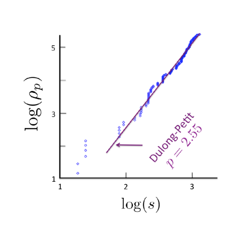
Figure 5: Entanglement spectrum. We extract the asymptotic behavior of the entanglement density of states $\rho_{p}$, for the first excited state of the five hexagon cluster of Fig. 3. The line depicts a pure power law at large pseudoenergies $s$, consistent with the Dulong-Petit form given in Eq. (11).

In Figure 5, we plot the entanglement spectrum for the first excited eigenstate of the 30 site, five hexagon Kagomé cluster depicted in Figure 3. The log-log plot demonstrates the asymptotic power law density of states $\sim s^{p}$, where $p\approx 2.55$. We note that for this system we are in the low $S_{ee}$ regime and hence the difference between the fitted value of $p+1$ and the entanglement entropy of $1.27$. Nevertheless, the density of states at high pseudo-energies extrapolates well to the asymptotic power law behavior of a classical gas as modelled in this section.

IV Implementation of the Lanczos-SVD iteration

The Lanczos-SVD routine proceeds as follows: We initialize $|\psi\rangle^{(0)}$ as a direct product of the two subcluster states. We compute $({\cal P}_{\rm{\rm{svd}}}H)^{n}|\psi^{(0)}\rangle=|\psi^{(n)})$ as described above. Since our method is economical in memory, we can afford to retain $L$ sequential Lanczos vectors $|\psi^{(n)}),|\psi^{(n+1)}),\ldots|\psi^{(n+L)})$, which speeds up the convergence with iteration number considerably. (If memory is scarce, one could use the slower method of keeping only two Lanczos vectors).

Now, we compute the overlap matrix and orthonormalize this set of Lanczos vectors. This produces a ”rotating basis” of dimension $L$

$$|\varphi^{(i)}\rangle=\sum_{n^{\prime}=n}^{n+L}A_{in^{\prime}}|\psi^{(n^{\prime})}\rangle,~{}~{}~{}~{}\langle\varphi^{(i)}|\varphi^{(j)}\rangle=\delta_{ij},$$ (16)

where $A$ are the coefficients determined by diagonalizing the overlap matrix (see e.g. Eq. (6)).

Subsequently, we compute the matrix elements of the reduced Hamiltonian,

$$H_{ij}=\langle\varphi^{(i)}|H|\varphi^{(j)}\rangle,~{}~{}~{}~{}i,j=1,\ldots L.$$ (17)

The reduced Hamiltonian matrix is diagonalized. Its lowest eigenvalue and eigenvector yield the best approximation to the ground state at this level of iteration weinsteincoreprd1993 . We bring the resulting wavefunction to the SVD form, again truncated into $n_{\rm{\rm{svd}}}$ terms. It becomes the new initial state $|\psi^{(n+L+1)}\rangle$ for the next Lanczos iteration. Excited states can be calculated by starting with an initial state orthogonal to the converged lower energy states.

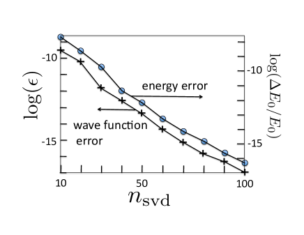
Figure 6: Lanczos-SVD truncation errors, for the 24 sites Kagomé cluster of Fig. 1. $n_{\rm{\rm{svd}}}$ is the number of retained SVD states of the ground state (3). $\epsilon$ is the wavefunction error Eq. (2) and following text). $\Delta E_{0}/E_{0}$ is the relative error in the the Lanczos-SVD ground state energy as compared to the exact (standard Lanczos) result. The rapid decay of the errors for low values of $n_{\rm{\rm{svd}}}<<2^{12}$ is due to the low entanglement entropy, see Section III.

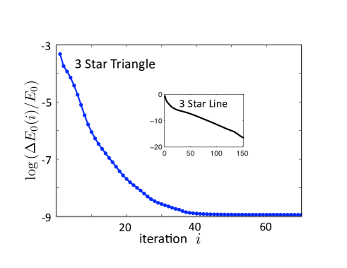
Figure 7: Lanczos-SVD error convergence as a function of iteration, for 36 site Kagomé clusters. The main plot is for Fig. 4, and the inset is for Fig. 2. $\Delta E_{0}(i)$ is difference between the energy at iteration $i$ and the converged ED result given by standard Lanczos sylvain36 . For both clusters we used $n_{\rm{svd}}=200$ and $L=4$ Lanczos vectors.

V Numerical tests

For the spin-half Heisenberg antiferromagnet

$$H=\sum_{\langle ij\rangle}{\bf S}_{i}\cdot{\bf S}_{j},$$ (18)

we tested the convergence of the Lanczos-SVD algorithm on Kagomé clusters depicted in Figs. 1, 2, 3 and 4.

In Fig. 6, we plot the Lanczos-SVD truncation error for the ground state wave function and energy, as a function of $n_{{\rm svd}}$. The errors decrease rapidly on the logarithmic scale as expected by Eq. (LABEL:error-est), arriving at $\approx 10^{-13}$ for $n_{{\rm svd}}=200$.

For the 30 site Kagomé cluster depicted in Fig LABEL:30sites, the energies of the four lowest S=0 eigenstates, and the first triplet S=1 state, converged to a very high accuracy of $10^{-11}$ using $n_{{\rm svd}}=200$.

In Fig.  7 we show the convergence of ground state energy of Lanczos-SVD versus iteration for clusters of 36 sites. We use $n_{\rm{\rm{svd}}}=200$, and $L=4$. For the three star triangle, the exact ground state energy as determined by standard Lanczos is $E_{0}(36{\rm{sites}})=-14.859397$ sylvain36 . The entanglement entropy is $S_{ee}\approx 2.5$. The calculation converges to relative energy accuracy of $1.3\times 10^{-4}$, and an SVD truncation error of similar magnitude.

In the inset of Fig. 7 we show a much smaller error for the three star line of Fig. 2, which converged to a relative error of $6.3\times 10^{-8}$. This is to be expected since the entanglement entropy of the linear arrangement of the three stars is only $S_{ee}\approx 1.12$.

The numerical tests were therefore consistent with Eq  (15).

All the above calculations were performed using multi-core workstations. The maximum memory usage was kept under 15 GB of memory, even though no lattice symmetries were implemented in the computations. The time required for the most intensive calculations (36 sites, $n_{{\rm svd}}=200$) on using parallelisation with 16 cores was a little more than 70 minutes per iteration Fig 4 and about 35 minutess for Fig. 2. A serial MAPLE 15 implementation used in the computations for the 30 site case took about one day for each eigenstate for the same $n_{{\rm svd}}$.

VI Extension to multiple partitioning of large lattices.

The Lanczos-SVD compresses the memory requirement by a single division of the cluster into two subclusters $i=1,2$. This idea could be extended to recursive partitioning mera-prl . For the sake of crude memory estimation, each small vector (e.g. $|\alpha\rangle_{i}$ in Eq. (1) can be decomposed into $n_{{\rm svd}}$ products of even smaller subcluster vectors. If the SVD is thus iterated $p$ times, one obtains a representation in terms of small vectors of $P=2^{p}$ subclusters. $|\psi\rangle$ is thus stored in terms of a set of the smallest vectors. The memory cost after applying a Lanczos step is as follows.

For concreteness, let us consider a two dimensional disk of radius $R>>1$, containing $N\simeq\pi R^{2}$ sites of spin half, divided into $P$ equal sections as shown in Fig.8. The sections are labeled by a binary number ${{\bf i}}=(i_{1},i_{2},\ldots i_{p})$, $i_{k}=0,1$. The recursive SVD decomposition yields the expression

$$|\psi\rangle=\sum_{\alpha_{1},\alpha_{2}\ldots\alpha_{p}}\lambda_{\alpha_{1}}\lambda^{i_{1}}_{\alpha_{1},\alpha_{2}}\cdot\cdot\lambda^{i_{1},\ldots i_{p-1}}_{\alpha_{1},\ldots\alpha_{p}}\prod_{{{\bf i}}}|\alpha_{1},\ldots\alpha_{p}\rangle_{{{\bf i}}}.$$ (19)

The SVD weights $\lambda^{{{\bf i}}}$ are labeled according to the boundaries they describe, as shown in Fig. (8). Each $\alpha_{i}$ runs over $n_{{\rm{svd}}}$ numbers, which means that each section ${\bf i}$ is represented by $n_{{\rm{svd}}}^{p}$ vectors of dimension $2^{N/P}$. By the ”area law” $S_{ee}\propto R$ on each boundary. As shown before, we must retain $n_{{\rm svd}}\sim e^{cR}$ terms in each SVD, where $c(\epsilon)>1$ in order to achieve a desired truncation error $\epsilon$.

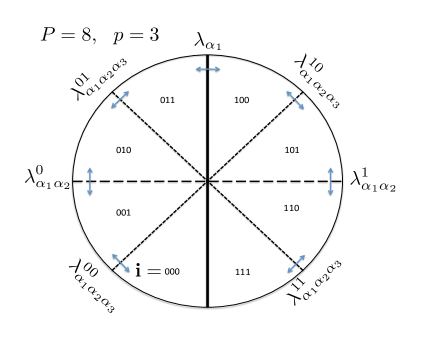
Figure 8: Multiple subclusters

After applying $H$ to $|\psi\rangle$, we generate a factor of $M\approx 6R$ more small vectors. Thus we should store $6PRn_{\rm{svd}}^{p}$ small vectors. Thus the memory cost is

$${\cal M}_{c}\approx 6PR\exp\left({cR\log(P)}+{\pi R^{2}\log(2)\over P}\right).$$ (20)

Minimizing ${\cal M}_{c}(P)$ one finds the optimal partitioning $P^{opt}$, and the optimal memory cost ${\cal M}^{opt}$ at large $N$ to scale as

$$P^{opt}\approx{\pi\log(2)R\over c},~{}~{}~{}{\cal M}_{c}^{opt}\sim Ne^{{c\over 2}\left(\sqrt{N/\pi}\log(N/\pi)-2\right)}.$$ (21)

This would amount to a significant compression of memory as compared to standard Lanczos ${\cal M}\sim 2^{N}$. The remaining challenge is to speed up the significantly larger computational time needed to orthonormalize and SVD large sets of small vectors.

VII Discussion

In this paper we have exploited the SVD to expand the lattice sizes which can be treated by the Lanczos algorithm for ED. Relative to standard Lanczos, Lanczos-SVD demands longer computation time due to additional matrix manipulations.

Does the SVD projection interfere with the Lanczos convergence?. The SVD projection introduces a truncation error in the rotating vector. However, the Lanczos vector is rotated toward the ground state (or some other target state) when the relative energy splitting to neighboring eigenstates is larger than the truncation error. This rotation ceases once the energy has converged within the SVD error. Increasing $n_{{\rm svd}}$ will allow further convergence. It is simplest to think about the SVD projection in the same footing as an additional floating point error which limits the numerical convergence of standard Lanczos algorithms. In computing Fig. 7 we have indeed verified that the implementation of SVD projection in each iteration, does not slow down the energy convergence per each Lanczos step.

Computing time of Lanczos-SVD may be significantly reduced by using multiple cores and by parallelizing the code. In particular the overlap calculations, which are currently the most time-consuming, are easily parallelizeable. In standard Lanczos, memory reduction can be achieved by exploiting lattice and spin symmetries, which demands special boundary conditions and extensive programming. Lanczos-SVD is therefore simpler to implement, and can address arbitrary boundary conditions.

It is often asked what advantage a Lanczos based ED has over DMRG and related variational methods? The answer of course depends on the purpose of the calculation. DMRG has proven very efficient (especially for ground state correlations) for larger lattices than Lanczos methods can address. However, in practical applications, DMRG advances toward the ground state by sequential minimizations, e.g. ”sweeping” the parameters of the wave function in real space. In cases of high frustration and competing phases (e.g. near a phase transition), sweeping methods can get stuck in metastable states DMRG2D . (Consider e.g. the difficulty of getting rid of defects in a phase separated system by sweeping methods).

The Lanczos step, on the other hand, does not necessarily move the state in the direction of maximal slope. Instead, if numerical accuracy is sufficient, it steadily rotates the Lanczos vector toward the true ground state (or some other target eigenstate).

Lanczos-SVD can therefore be used to determine the ground state and low excitations of limited size clusters with well controlled accuracy. It could be used to check DMRG convergence and test variational ansatzes. As mentioned in the introduction, a primary purpose for using ED on small clusters is to derive an effective Hamiltonian by the CORE methodCORE-future . The CORE effective Hamiltonian can then be studied on the coarse grained lattice by iterating CORE, or by variational methods.

Acknowledgments

We thank Dan Arovas, Yosi Avron, Sylvain Capponi, Steve Kivelson, Israel Klich, Netanel Lindner and Steve White for insightful conversations. AA acknowledges support from Israel Science Foundation, and US-Israel Binational Science Foundation, and the hospitalilty of Aspen Center For Physics.

References

- (1) C. J. Morningstar, M. Weinstein Phys.Rev. D 54, 4131 (1996); Marvin Weinstein Phys.Rev. B63, 174421 (2001); M.Stewart Siu, Marvin Weinstein Phys. Rev. B 77, 155116 (2008).
- (2) E. Altman and A. Auerbach, Phys. Rev. B 65, 104508 (2002); E. Berg, E. Altman, and A. Auerbach, Phys. Rev. Lett. 90, 147204 (2003); R. Budnik and A. Auerbach Phys. Rev. Lett. 93, 187205 (2004).
- (3) S. Capponi, A. Läuchli, and M. Mambrini Phys. Rev. B 70, 104424 (2004).
- (4) For recent advances in ED on large Kagomé clusters see A.M. Läuchli, J. Sudan, E.S. Sorensen, arXiv:1103.1159.
- (5) N. H. Lindner and A. Auerbach, Phys. Rev. B 81, 054512 (2010).
- (6) J. E. Avron and R. Seiler, Phys. Rev. Lett. 54, 259 (1985); N. Lindner, A. Auerbach, D. P. Arovas, Phys. Rev. B 82 134510 (2010).
- (7) C. Lanczos. J. Res. Nat. Bur. Stand 45, 255 (1950)
- (8) J. K. Cullum and R. A. Willoughby, Lanczos Algorithms for Large Symmetric Eigenvalue Computations, Birkhuser (1985)
- (9) L. Amico, R. Fazio, A. Osterloh, and V. Vedral, Rev. Mod. Phys. 80, 517 (2008) (and references therein).
- (10) F. Verstraete, M. A. Martin-Delgado, and J. Cirac, Phys. Rev. Lett. 92, 087201 (2004).
- (11) M. B. Hastings,Phys. Rev. B 69, 104431 (2004);
- (12) E. Fradkin, and J. E. Moore, Phys. Rev. Lett. 97, 050404 (2006).
- (13) I. Klich, G. Refael, and A. Silva, Phys. Rev. A 74, 032306 (2006).
- (14) S. R. White, Phys. Rev. Lett. 69, 2863 (1992); Phys. Rev. B 48, 10345 (1993).
- (15) S. Ostlund and S. Rommer, Phys. Rev. Lett. 75, 3537 (1995).
- (16) T. Papenbrock and D. J. Dean, Phys.Rev. C 67 051303 (2003).
- (17) G. Vidal, Phys. Rev. Lett. 99, 220405 (2007); L. Tagliacozzo, G. Evenbly, and G. Vidal, Phys. Rev. B 80, 235127 (2009); G. Evenbly and G. Vidal, Phys. Rev. Lett. 104, 187203 (2010).
- (18) A power law can fit the numerical entanglement spectra asymptotics of two dimensional systems computed by e.g. M-C. Chung and I. Peschel , Phys. Rev. B 64, 064412 (2001). H. Li and F. D. M. Haldane, Phys. Rev. Lett. 101, 010504 (2008).
- (19) M. Weinstein, Phys. Rev. D 47, 5499 (1993).
- (20) S. Capponi, Private communication
- (21) E.M. Stoudenmire and Steven R. White, arXiv:1105.1374v2.
- (22) A. Auerbach, S. Capponi, V. Ravi Chandra and M. Weinstein,(unpublished).