Probing the initial conditions of high-mass star formation – II

Most work on high-mass star formation has focused on observations of young massive stars in protoclusters. Very little is known about the preceding stage. Here, we present a new high-resolution study of pre-protocluster regions in tracers exclusively probing the coldest and dense gas ($\rm NH_{2}D$). The two target regions G29.96$-$0.02 and G35.20$-$1.74 (W48) are drawn from the SCAMPS project, which searches for pre-protoclusters near known ultracompact Hii regions. We used our data to constrain the chemical, thermal, kinematic, and physical conditions (i.e., densities) in G29.96e and G35.20w. $\mathrm{NH_{3}}$, $\mathrm{NH_{2}D}$, and continuum emission were mapped using the VLA, and PdBI. In particular, $\mathrm{NH_{2}D}$ is a unique tracer of cold, precluster gas at high densities, while $\mathrm{NH_{3}}$ traces both the cold and warm gas of modest-to-high densities. In G29.96e, Spitzer images reveal two massive filaments, one of them in extinction (infrared dark cloud). Dust and line observations reveal fragmentation into multiple massive cores strung along filamentary structures. Most of these are cold ($<20\leavevmode\nobreak\ \rm K$), dense ($>10^{5}\leavevmode\nobreak\ \rm cm^{-3}$) and highly deuterated ([$\mathrm{NH_{2}D}$/$\mathrm{NH_{3}}$]$>6\%$). In particular, we observe very low line widths in $\mathrm{NH_{2}D}$ (FWHM $\lesssim 1\leavevmode\nobreak\ \rm km\,s^{-1}$). These are very narrow lines that are unexpected towards a region forming massive stars. Only one core in the center of each filament appears to be forming massive stars (identified by the presence of masers and massive outflows); however, it appears that only a few such stars are currently forming (i.e., just a single Spitzer source per region). These multi-wavelength, high-resolution observations of high-mass pre-protocluster regions show that the target regions are characterized by (i) turbulent Jeans fragmentation of massive clumps into cores (from a Jeans analysis); (ii) cores and clumps that are “over-bound/subvirial”, i.e. turbulence is too weak to support them against collapse, meaning that (iii) some models of monolithic cloud collapse are quantitatively inconsistent with data; (iv) accretion from the core onto a massive star, which can (for observed core sizes and velocities) be sustained by accretion of envelope material onto the core, suggesting that (similar to competitive accretion scenarios) the mass reservoir for star formation is not necessarily limited to the natal core; (v) high deuteration ratios ([$\mathrm{NH_{2}D}$/$\mathrm{NH_{3}}$]$>6\%$), which make the above discoveries possible; (vi) and the destruction of $\mathrm{NH_{2}D}$  toward embedded stars.

1 Introduction

High-mass stars are known to form in clusters and, given their rarity, most such clusters have typical distances of a few kpc or greater. In spite of being few in number relative to solar-mass stars, high-mass stars play a large role in shaping the Galaxy in each of their evolutionary stages, with energetic stellar winds, powerful outflows, UV radiation, expanding Hii regions, and finally supernova explosions. Observations until perhaps the last decade were hindered by a lack of sensitivity and resolution, crucial for such regions, which are more crowded and farther away than typical low-mass star-forming regions.

With the development of infrared sky surveys (starting with IRAS, then ISO, MSX, and recently Spitzer) and sensitive ground-based mm/submm bolometer observations the potential early phases in the formation of high-mass stars/clusters have been identified.

Combining these results with higher angular resolution follow-up observations with radio interferometers yields a suggested evolutionary sequence that separates the actively accreting high-luminosity protostars in clusters with no cm continuum (high-mass protostars $\rightarrow$ hot molecular cores in protoclusters) from those with cm continuum (hypercompact and ultra-compact Hii regions: see Beuther et al. 2007 for a review).

The earliest stage in this scenario would be a “pre-protocluster stage”, which is harder to find. The properties of this precluster stage sets the initial conditions for the formation of high-mass stars. Observers have attempted to identify candidate pre-protocluster cores in many different ways (Hill et al. 2005, Sridharan et al. 2005, Rathborne et al. 2006, Pillai et al. 2007). Follow ups with outflow tracers combined with sensitive Spitzer observations have however revealed active star formation in many of these cores (for e.g. Rathborne et al. 2005, Pillai et al. 2006b, Beuther & Steinacker 2007). A frequently used way of identifying the precluster phase has been to scan the infrared data for dark absorption features against the bright mid-infrared background. Several thousand such dark clouds, now commonly known as infrared dark clouds (IRDCs: Egan et al. 1998, Simon et al. 2006, Peretto & Fuller 2009) have been identified along the Galactic Plane. One of the filaments studied in this paper is such an IRDC.

To our knowledge, interferometer observations on the high-mass precluster phase (as opposed to protocluster phase) in dense gas tracers have been few (Swift 2009, Zhang et al. 2009b, Busquet et al. 2010). The few interferometer observations that have been done focused on the dust continuum structure or the chemistry. The dust continuum is expected to be weak at these scales (as opposed to the strong dust continuum from the envelope as observed by single dishes). This is because precluster phase is colder and less concentrated than the protocluster phase, and therefore such observations often detect only the protoclusters. Therefore, until the commissioning of ALMA, we have to rely on molecular observations that trace the dense and cold gas. Ammonia and $\mathrm{N_{2}H^{+}}$ has proven to be an important tool in measuring the physical conditions in the prestellar stages (Tafalla et al., 2002). These molecules do not deplete from the gas phase for the high densities ($<10^{6}$ $\mathrm{cm^{-3}}$) and cold temperatures ($<20$ K) expected in the prestellar stages. Emission from deuterated analogues ($\mathrm{NH_{2}D}$, and $\mathrm{N_{2}D^{+}}$) of these two molecules is sensitive not only to dense, but also very cold gas. Warmer temperatures ($>20$ K) usually inhibit deuterium enhancement (see Bergin & Tafalla 2007 for a review of chemistry in dark clouds).

We embarked on a project to identify this very early stage in the formation of a high-mass star. We identified secondary high-mass cold cores in the close vicinity of UCHii regions in a SCUBA wide-field mapping survey of $10\times 10$ ′ (SCAMPS: the SCUBA Massive Pre/Protocluster core Survey; Thompson et al. 2005). Recently, we reported on a single dish study of $\mathrm{NH_{3}}$ deuteration ([$\mathrm{NH_{2}D}$/$\mathrm{NH_{3}}$]) and depletion (of CO) toward a sub-sample of these new massive pre/protocluster cores. More than half of the sources exhibit a high degree of deuteration ($0.1-0.7$). The enhancement in deuteration coincides with moderate CO depletion onto dust grains (Pillai et al., 2007). Here, we present interferometer observations of $\mathrm{NH_{3}}$ and $\mathrm{NH_{2}D}$ using the VLA, BIMA and PdBI for two sources from the SCAMPS project.

The SCAMPS source which we denote G29.96e in this paper, is an IRDC about two arcmin east of the ultracompact Hii region G29.96-0.02. The cometary Hii region itself is one of the brightest radio and infrared sources in our Galaxy, and has been studied in detail at infrared and radio wavelengths (Wood & Churchwell 1989, Pratap et al. 1999; Kirk et al. 2010). We adopt the kinematic distance of 7.4 kpc to the cloud estimated from the $\mathrm{NH_{2}D}$ LSR velocity.

The other SCAMPS source which we denote G35.20w lies about one arcmin west of the W48 Hii region (G35.20$-$1.74). We adopt a distance of 3.27 kpc based on recent trigonometric parallax measurements by Zhang et al. (2009a). This value is very close to our kinematic distance estimate of 3.4 kpc for the region. The position of the high-mass cloud we found with SCUBA roughly coincides with that of a molecular cloud adjacent to W48 region mapped at coarse resolution in CO, and its isotopomers (Vallee & MacLeod 1990, Zeilik & Lada 1978). This region has been studied in dust polarization by Curran et al. 2004, where our G35.20w is referred to as W48W.

By determining the properties of these massive secondary cores from our high angular resolution observations, we will constrain the initial conditions of high-mass star formation. After presenting the observations (Section 2), we will discuss our main results (Section 3), then analyze these results (Section 4), and finally discuss the relevance of these results in the context of current theories on initial fragmentation and collapse in high-mass star-forming regions (Section 5).

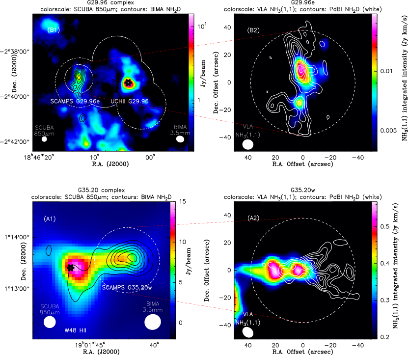
Figure 1: Overview of the SCAMPS regions, G29.96e (top) and G35.20w (bottom). Panel (A1): SCUBA 850$\mu$m dust continuum (color scale) and BIMA $\mathrm{NH_{2}D}$ at 85.9 GHz (contours).Panel (A2): VLA $\mathrm{NH_{3}}$ (1,1) (color scale) starting at 3$\sigma$ and PdB $\mathrm{NH_{2}D}$ at 85.9 GHz (white contours). Panel (B1): SCUBA 850$\mu$m dust continuum (color scale) and BIMA $\mathrm{NH_{2}D}$ at 85.9 GHz (contours). The white dash circle indicates the BIMA coverage. Panel (B2): VLA $\mathrm{NH_{3}}$ (1,1) integrated intensity (color scale) starting at 3$\sigma$ and PdB $\mathrm{NH_{2}D}$ at 85.9 GHz integrated intensity (white contours). The contour levels for PdBI maps start at $-3\sigma$, $3\sigma$ in steps of 3$\sigma$. The primary beam at 3.5 mm is indicated by white dashed circles in the right panels. The nominal positions of the Hii regions are marked as stars (Wood & Churchwell, 1989).

2 Observations

Here we describe the radio interferometer observations with various telescopes, in line and continuum, as well as the Spitzer archival data. All the figures shown in the paper (except for the first reference figure, figure 1) are with respect to the phase center of the Plateau de Bure Interferometer (PdBI) observations (Table 1). A summary of line and continuum frequencies relevant to this paper is given in Table 2. The final synthesized beam, as well as the root mean square (RMS) noise level for each set of observations is given in Table LABEL:tab:beam_rms.

Table 1: Reference Position for PdBI Interferometer Observations

Source	R.A.(J2000)	Dec.(J2000)	$v_{\rm LSR}$ [km/s]
G29.96e	18:46:12.78	$-$02:39:11.8	100.4
G35.20w	19:01:42.11	$+$01:13:33.4	42.4

The SCUBA observations have been reported in Thompson et al. 2005, and will be detailed in a separate paper (Thompson et al. in preparation).

Table 2: Relevant observed rotational transitions.

Species	Transition	Array	$\nu$ (MHz)
$\mathrm{NH_{2}D}$	111–101	PdBI	85926.3
$\mathrm{NH_{3}}$	(1,1)	VLA	23694.496
$\mathrm{NH_{3}}$	(2,2)	VLA	23722.633
$\mathrm{HCO^{+}}$	1–0	BIMA	89188.5230

2.1 PdBI observations

G29.96e and G35.20w were observed with the PdBI in its C and D configurations on Mar 27/28th and Apr 20/21st 2004. The 3.5 mm receivers were tuned to the $\rm NH_{2}D$ line at 86.086 GHz in single sideband mode. The 1.3 mm receivers were tuned to 219.560 GHz in DSB mode. The 3.5 mm lines were observed with a resolution of 80 kHz. At both wavelengths two 320 MHz wide correlator windows were used to probe the continuum emission. The spectral resolution for the $\mathrm{NH_{2}D}$ observations is $\approx 0.27$ $\mathrm{km\,s^{-1}}$.

Hexagonal mosaics with a spacing of 10 arcsec were used to increase the field of view. This kept the sensitivity at the mosaic center very high for the 3.5 mm observations and led to fully sampled mosaics at 1.3 mm.

Using natural weighting, the synthesized beam sizes, and sensitivities at 3 and 1.3mm are as given in Table LABEL:tab:beam_rms.

2.2 VLA observations

The 23 GHz $\mathrm{NH_{3}}$ observations are reported for two sources G35.20w and G29.96e. We retrieved the data for $\mathrm{NH_{3}}$ (1,1) and (2,2) transitions at 1.3 cm from the VLA archive toward G35.20w, while for G29.96e, we report new observations with the VLA.

The 23 GHz G29.96e $\mathrm{NH_{3}}$ observations were done with the Very Large Array (VLA) on 24 August 2004 in its D configuration and in 2 polarizations with a spectral resolution of 0.33 $\mathrm{km\,s^{-1}}$. The primary beam at 23 GHz is $\sim$2 arcmin. The observations were carried out in a three pointing mosaic covering the SCAMPS source G29.96e as well as the cometary Hii region G29.96$-$0.02. The standard interferometer mode was used with a total integration time of 20 minutes on source split into sessions. Phase calibration was done using J1733-130 and the flux calibrator was 3C286. The archival data retrieved for G35.20w were obtained in D array on 03 August 2000, covering the (1,1) and (2,2) lines with 2$\times$64 49 kHz channels. The phase center was at $\alpha_{\rm J2000}=$19:01:45.5, $\delta_{\rm J2000}=$$+$01:13:28.00. The total integration time on source was approximately 50 minutes. The phase calibrator J1824+107 was observed every 10 minutes and the flux calibrator was 3C286.

2.3 BIMA observations

G35.20w and G29.96e were observed with BIMA in its D configuration in Jul/Aug. 2003 in three tracks. The receivers were tuned to the $\rm NH_{2}D$ frequency. Simultaneously, HCO$+$ (1-0) was observed in the upper sideband. The frequency resolution was 0.1 MHz. More details on the observations are as given in Table LABEL:tab:beam_rms. Towards G29.96e, a 5 point mosaic was observed to cover both the hot core and the SCAMPS source in the east. Phase calibration with 1743-038 was performed every 15 minutes, and Uranus was observed as flux calibrator.

Table 3: The sensitivity and beam parameters for the interferometer observations. Columns are the interferometer used, the wavelength with the molecule in brackets for line observations, the effective beam, its position angle and the RMS noise level in the final image.

Instrument	Wavelength(type)	$\theta_{\rm maj}\times\theta_{\rm min}$	PA	RMS (type)
		arcsec	degrees	mJy/beam
		G29.96e
PdBI	1.3mm	2.2 $\times$ 1.6	44	2.3 (continuum)
	3.5mm ($\mathrm{NH_{2}D}$)	5.5 $\times$ 4.1	43	0.5 (continuum), 35 (line)
VLA	23.6 GHz ($\mathrm{NH_{3}}$)	8.0 $\times$ 7.4	12	1.1 (line)
BIMA	89.2 GHz (HCO$+$ 1–0)	21.7 $\times$ 17.6	14.3	420 (line)
		G35.20w
PdBI	1.3mm	1.8 $\times$ 1.7	52	2.5 (continuum)
	3.5mm ($\mathrm{NH_{2}D}$)	4.5 $\times$ 4.2	45	0.5(continuum), 31 (line)
VLA	23.6 GHz ($\mathrm{NH_{3}}$)	8.7 $\times$ 6.9	42	1.2 (line)
BIMA	89.2 GHz (HCO$+$ 1–0)	19.2 $\times$ 18.2	-20.6	210 (line)

2.4 Spitzer archival data

The Spitzer MIR data collected from the Spitzer data archive is part of the GLIMPSE (Benjamin et al. 2003; Churchwell et al. 2009, and MIPSGAL Legacy survey (Carey et al. 2009) in 4 of the Infrared Array Camera (IRAC) bands from $3.6$ to 8$\mu$m, and two of the Multiband Imaging Photometer (MIPS) bands at 24, and 70$\mu$m, respectively, These two Galactic Plane surveys cover the inner Galactic Plane, and thus include the G29.96e region but not G35.20w which lies outside the latitude limits of GLIMPSE & MIPSGAL. However, we were able to download the MIPS 24$\mu$m data for G35.20w from a dedicated survey of UCHII regions by Carey et al (Spitzer Program ID 20778). Our molecular cloud happened to be just within the 24$\mu$m field of view of their target, but the 70$\mu$m image did not cover this cloud.

We discuss G29.96e, followed by G35.20w in each subsection below.

3 Results

3.1 Methods

3.1.1 Identification of $\mathrm{NH_{3}}$ and $\mathrm{NH_{2}D}$ clumps

We used CLUMPFIND, a 3-dimensional clump finding algorithm, to identify the $\mathrm{NH_{2}D}$ cores (Williams et al., 1994). The threshold for $\mathrm{NH_{2}D}$ was set to $0.2\leavevmode\nobreak\ \rm Jy\,beam^{-1}$ for both sources. The step size was $0.02\leavevmode\nobreak\ \rm Jy\,beam^{-1}$, where the RMS noise level (measured in regions free of emission) is $35\leavevmode\nobreak\ \rm mJy\,beam^{-1}$. For $\mathrm{NH_{3}}$ observations of G29.96e, the threshold was set to $0.005\leavevmode\nobreak\ \rm Jy\,beam^{-1}$, and we used an increment of $0.001\leavevmode\nobreak\ \rm Jy\,beam^{-1}$. For G35.20w in this line, a higher threshold of $0.02\leavevmode\nobreak\ \rm Jy\,beam^{-1}$ was used, while the step size was lowered to an unusually low value (a fraction of the threshold value), in order to separate two equal intensity peaks. The observed transition with six hyperfines can be grouped into three pairs: a main pair hfs_mg(which are blended), an inner pair hfs_in, and an outer pair hfs_out. We ignored the outer hyperfines and considered the whole velocity range within the inner hyperfines in CLUMPFIND, since in LTE hfs_out are only 30% as bright as the main group. We identified 11 clumps in G29.96e and 13 in G35.20w. The clumps are referred to as P1…P’n’ (n=11 for G29.96e, and n=13 for G35.20w) in Table 4. Similarly, we identified 5 and 3 $\mathrm{NH_{3}}$ clumps in G29.96e and G35.20w respectively. The line parameters for $\mathrm{NH_{3}}$ clumps are listed in Table 5.

3.1.2 Identification of PdBI dust continuum cores

A modified version of CLUMPFIND for 2-dimensional data is available. However, on manually checking the results, we found that the structures were not intuitively meaningful in some cases. Therefore, we chose to identify dust emission cores as dust emission peaks of an intensity that exceeds the noise level by at least a factor 5 and with sizes larger than a beam. We assigned masses to them according to the following scheme. For a given core (i.e., peak), we identify the $3\leavevmode\nobreak\ \sigma$ contour that contains this core. If this contour contains a single peak, then all of the area contained within the $3\leavevmode\nobreak\ \sigma$ contour is assigned to that core. If several cores are present within the contour, then the core boundaries are drawn at the saddle points separating these cores, respectively at the $3\leavevmode\nobreak\ \sigma$ contour enveloping the peaks. The dust continuum mass is then computed over an effective area of radius R_eff after a beam deconvolution. Results are presented in Table 6.

3.1.3 Analysis of $\mathrm{NH_{3}}$ and $\mathrm{NH_{2}D}$  spectra

To determine the gas temperature and column density, we followed the analysis routine described in Pillai et al. (2007). The ratio of the brightness temperatures of the $\mathrm{NH_{3}}$ (1,1) and (2,2) transitions, along with the optical depth, can be used to estimate the rotational temperature. For temperatures $<20\leavevmode\nobreak\ \rm K$, which are typical of cold dark clouds, the rotational temperature closely follows the gas kinetic temperature (Walmsley & Ungerechts, 1983). Like $\mathrm{NH_{3}}$(1,1) and (2,2), its isotopologue $\mathrm{NH_{2}D}$ 1₁₁–1₀₁ also has hyperfines. This allows the estimation of optical depth and hence the column density of $\mathrm{NH_{2}D}$. We estimate the $\mathrm{NH_{3}}$ column density assuming that the level populations are thermalized, i.e., $T_{\rm ex}=T_{\rm rot}$. A similar assumption holds for our estimation of $\mathrm{NH_{2}D}$ column densities. i.e., Assuming that $\mathrm{NH_{2}D}$ and $\mathrm{NH_{3}}$ reside in the same volume, the excitation of $\mathrm{NH_{2}D}$ can be gauged using the gas temperatures derived from the $\mathrm{NH_{3}}$ analysis. This permits to derive $\mathrm{NH_{2}D}$ column densities. The expressions used to estimate the $\mathrm{NH_{2}D}$ column density from the radiative transfer equation is given in Appendix A of Pillai et al. (2007). We derive the $\mathrm{NH_{2}D}$ column density solely based on the ortho transition. For this, we assume that the ortho and para transitions are in LTE. The $\mathrm{NH_{2}D}$ partition function is determined by considering the contribution of the different energy levels from $J=0$ to $J=2$. Then, the $\mathrm{NH_{2}D}$ and $\mathrm{NH_{3}}$ fractionation ratio can be calculated from ratios of column densities. We calculate the line parameters (line width, peak brightness, LSR velocity) for both tracers for the same beam size, averaged over a square aperture of size equal to the beam major axis. We then estimate the deuteration ratio [$\mathrm{NH_{2}D}$/$\mathrm{NH_{3}}$] wherever both tracers are detected with a signal that exceeds the noise level by a factor 3. We require that the uncertainties in their ratios are below 50%. Table 5 lists our results.

3.1.4 Mass determination

We derive the gas mass from the 1.3 mm and 3.5 mm dust continuum emission for the different clumps identified at both wavelengths following Kauffmann et al. (2008), using dust opacities at 1.3 mm (0.009 $\rm cm^{2}/g$) and 3.5 mm opacities (0.002 $\rm cm^{2}/g$) for dust grains with thick ice mantles and gas density $\rm n(H)=10^{6}\leavevmode\nobreak\$$\mathrm{cm^{-3}}$as in Ossenkopf & Henning 1994, and gas to dust ratio of 100. A dust opacity index of 1.61 is obtained by interpolating between two nearest wavelengths 1.075 mm and 1.300 mm from Ossenkopf & Henning (1994). Here, we adopt dust temperatures identical to the $\mathrm{NH_{3}}$-derived ones (Table 5). If no such measurement exists, a temperature of $16\leavevmode\nobreak\ \rm K$ is used. This is the case for e.g. when the $\mathrm{NH_{3}}$ temperature measurements have a large ($>$30%) error. We adopt $16\leavevmode\nobreak\ \rm K$ since it is the average temperature of the cores (Table 5). For a temperature of 16 K, the 1.3 mm continuum sensitivity limit quoted in Table LABEL:tab:beam_rms correspond to a mass limit of $\sim 4$ and $1\,M_{\sun}\,\rm beam^{-1}$ for G29.96e and G35.20w, respectively.

3.2 Overall cloud structure and associated star formation

3.2.1 G29.96e

We discovered the molecular clump G29.96e in our SCAMPS $10\arcmin\times 10\arcmin$ wide-field mapping survey of the G29.96-0.02 region as the brightest dust clump that has no associated $8\leavevmode\nobreak\ \rm\mu m$ infrared emission (as seen with MSX). The SCUBA map exposes G29.96e as an elongated feature that is dominated by a single bright peak (Fig. 1). The estimated total mass of this region, estimated from SCUBA data, is $7000\,M_{\sun}$ (Sect. 4.4). The PdBI map at $3\leavevmode\nobreak\ \rm mm$ wavelength shows a filament of about $1\arcmin$ ($\sim 2\leavevmode\nobreak\ \rm pc$) length that runs north-south. CLUMPFIND breaks this emission up into 3 cores. At even higher spatial resolution, the $1\leavevmode\nobreak\ \rm mm$ PdBI map reveals seven cores with a mass of $58\leavevmode\nobreak\ {\rm to}\leavevmode\nobreak\ 320\,M_{\sun}$ and a radius $\sim 0.1\leavevmode\nobreak\ \rm pc$ (Sect. 4.4). We denote these cores as mm1 to mm7 (the cores from the $3\leavevmode\nobreak\ \rm mm$ remain unnamed), in order of decreasing peak intensity (Table 6).

The Spitzer $8\leavevmode\nobreak\ \rm\mu m$ image of G29.96e, shown in Fig. 3, reveals this region as an Infrared Dark Cloud (IRDC); it is seen in extinction against the Galactic background. The extinction features correlate strongly with the PdBI continuum emission. Such extinction structures are still visible in Spitzer images at $24\leavevmode\nobreak\ \rm\mu m$ wavelength (also shown in Fig. 4). The latter images also expose a point source in this region, coincident with the dust core G29.96e mm1. This source drives an outflow at a velocity similar to one of the G29.96e clumps (see below). This kinematic information suggests that the $24\leavevmode\nobreak\ \rm\mu m$ point source is physically associated with the G29.96e region (i.e., does not reside in the foreground or background). The core G29.96e mm1 is therefore apparently actively forming stars or clusters. The Spitzer $8\leavevmode\nobreak\ \rm\mu m$ images arguably show an elongated bright structure towards G29.96e mm1; this may be due to emission from an outflow (e.g. Shepherd et al. 2007). No star-formation activity is detected in other parts of the cloud. Walsh et al. (1998) have reported a Class II methanol maser detection at 6.7 GHz towards G29.96e ($\sim 4$ ″north offset from G29.96e mm1). These masers are exclusive signposts of the earliest stages of high-mass star formation (Pestalozzi et al., 2007).

The wide-field map from BIMA shows that $\mathrm{NH_{2}D}$ is only detected towards the G29.96e region, and not towards the neighboring G29.96-0.02 Hii region (see Fig.1). This is consistent with the picture of G29.96e being colder than clump that hosts the Hii region: high temperatures are expected to yield low abundances of $\mathrm{NH_{2}D}$ (Sect. 4.3.1). The PdBI maps probe the $\mathrm{NH_{2}D}$ distribution at higher spatial resolution. Segmentation of the map with CLUMPFIND yields 11 cores. There is a very good correlation between the PdBI-observed $\mathrm{NH_{2}D}$ and dust emission distribution, as well as the Spitzer $8\leavevmode\nobreak\ \rm\mu m$ extinction structures. Details of this spatial correlation are examined in Sect.4.3. We also smooth the PdBI $\mathrm{NH_{2}D}$ maps to the resolution of the VLA $\mathrm{NH_{3}}$ data, in order to compare their distribution. This reveals a strong correlation between $\mathrm{NH_{2}D}$ and $\mathrm{NH_{3}}$; however, we do also find two $\mathrm{NH_{3}}$ cores without $\mathrm{NH_{2}D}$ emission (for e.g. those at $[+5,-29]$ and $[-16,+28]$). The $\mathrm{NH_{2}D}$ emission is well within the VLA primary beam (2 ′) at 23 GHz. Such details are also further examined in Sect.4.3. The $\mathrm{NH_{3}}$ analysis yields rotational temperatures (which serve as an estimate of the kinematic temperatures) of $13\leavevmode\nobreak\ {\rm to}\leavevmode\nobreak\ 23\leavevmode\nobreak\ \rm K$.

BIMA maps in the $\mathrm{HCO^{+}}$ (1–0) line reveal emission from one or several outflows. This is shown in Fig.2, where we present integrated intensity maps for the blueshifted (91–96.0 $\mathrm{km\,s^{-1}}$) and the redshifted (from 108–112 $\mathrm{km\,s^{-1}}$) outflow emission. Both velocity-integrated signals peak at opposite sides of G29.96e mm1, which suggests that the outflow source resides in this core. Broad line wings are also observed with the SMA in the CO (3–2) transition. A detailed characterization of the outflows and the massive protocluster in G29.96e mm1 will be presented in a future paper.

3.2.2 G35.20w

The clump G35.20w was found in our SCAMPS SCUBA survey map of the W48 Hii, where it manifests as a dust filament with east-west orientation that points away from the Hii region (Fig.1). Another filament with north-south orientation is detected closer to W48; this structure is not further examined here. The G35.20w filament has a physical size of $\sim 2\leavevmode\nobreak\ \rm pc$, slightly shorter than the length of the filament in G29.96e as observed with SCUBA. The SCUBA map reveals a filamentary structure in G35.20w: the field studied here contains four peaks. The total mass of the filament from the SCUBA data is $\sim 5000\,M_{\sun}$ (see Sect.4.4 for aperture and core masses). The 3.5 mm PdBI dust emission map essentially recovers the filamentary structure already seen with SCUBA, but shows it at higher spatial resolution. The 1.3 mm dust map from the PdBI, however, only reveals 4 compact peaks in the map, i.e. the global filamentary structure is lost because of interferometer filtering. Compared to G29.96e, this filtering is stronger in G35.20w, since the latter source is closer and thus larger when projected onto the sky. The compact 1.3 mm dust emission cores, numbered mm1 to mm4, have a radius $\sim 0.02\leavevmode\nobreak\ \rm pc$ and a mass of $8\leavevmode\nobreak\ {\rm to}\leavevmode\nobreak\ 18\,M_{\sun}$. This is much denser and the radii and masses smaller than in G29.96e. Different physical domains are thus probed in G29.96e and G35.20w.

Unfortunately, neither GLIMPSE nor MIPSGAL data are currently available for G35.20w, being at a Galactic latitude above the range covered by either surveys. As mentioned in Sect. 2.4, we were able to download the MIPS 24 $\mu$m data for G35.20w from a dedicated survey of UCHii regions by Carey et al (Spitzer Program ID 20778). Our molecular cloud happened to be just within the 24 $\mu$m field of view of their target, but the 70 $\mu$m image did not cover this cloud. The SCUBA clump (which is resolved into “streamers” at higher resolution) appears to originate right at the edge of the strong MIR emission of the W48 Hii region. Our brightest mm continuum source, G35.20w mm1, is associated with bright point-like emission at 24$\mu$m. A comparison of Spitzer and $\mathrm{NH_{2}D}$ in Sect. 4.3.2 shows no MIR emission associated with $\mathrm{NH_{2}D}$ in G35.20w. 6.7 GHz Class II methanol masers have been detected significantly offset from the streamer, closer to the Hii region (Goedhart, Wyrowski & Gibb in preparation). These masers are exclusive signposts of the earliest stages of high-mass star formation (Pestalozzi et al., 2007). However unlike in G29.96e, the gas streamer seen in $\mathrm{NH_{2}D}$  and dust continuum is not seen in absorption (nor in emission) against the MIR background. This is likely because the star-forming region itself is slightly below the Galactic Plane which usually provides the bright MIR background which the cold dust would absorb, and be seen as IRDCs.

In the BIMA wide-field mapping, $\mathrm{NH_{2}D}$ is clearly detected in G35.20w, but only a weak detection is found towards the north-south dust filament closer to W48 (Fig.1). Given our present understanding of deuteration fractionation (Sect.4.3), G35.20w is thus supposedly less evolved than the other filament. The PdBI data reveal several $\mathrm{NH_{2}D}$ filaments. CLUMPFIND segments these into 12 cores. The $\mathrm{NH_{2}D}$ emission is strongly correlated with the filamentary dust emission, as probed at 3.5 mm wavelength. This correlation is, however, weaker than in G29.96e: it is actually rather poor in the eastern part of G35.20w. In that region, a weak correlation is also observed between $\mathrm{NH_{2}D}$ and the VLA-probed $\mathrm{NH_{3}}$ emission. Conversely, the western part of G35.20w hosts $\mathrm{NH_{2}D}$ cores not seen in $\mathrm{NH_{3}}$ map. This is not surprising because these are the only $\mathrm{NH_{2}D}$ cores that lie outside the primary beam of the VLA. Such details of the $\mathrm{NH_{2}D}$ data are also examined in Sect.4.3. The $\mathrm{NH_{3}}$ emission, in contrast, correlates well with the 3.5mm dust emission. We derive rotational temperatures of $15\leavevmode\nobreak\ {\rm to}\leavevmode\nobreak\ 21\leavevmode\nobreak\ \rm K$ from analysis of the $\mathrm{NH_{3}}$ emission.

BIMA $\mathrm{HCO^{+}}$ (1–0) maps reveal an outflow in G35.20w, just as observed in G29.96e. The distribution of the velocity-integrated blueshifted (25.5 – 35.0 $\mathrm{km\,s^{-1}}$) and redshifted (46.6 – 53.6 $\mathrm{km\,s^{-1}}$) emission is presented in Fig.2. The core G35.20w mm1 is located in between the intensity maxima of these two velocity maxima, and so it is likely the source of the outflow. This core is thus actively forming a star or cluster. Detailed studies of this object are not the focus of the present paper, though. Signs for active star formation are detected nowhere else in the field studied here.

Table 4: Line parameters, and virial mass for $\mathrm{NH_{2}D}$ cores.

Core	Offsets	$v_{\rm LSR}$	$\Delta$va	$\tau_{\rm tot}$b	Reff	Mvirc	Mdustc	$\alpha$d	$\rho$e
	arcsec	$\mathrm{km\,s^{-1}}$	$\mathrm{km\,s^{-1}}$		parsec	$\hbox{M}_{\odot}$	$\hbox{M}_{\odot}$		105($\mathrm{cm^{-3}}$)
			G29.96e
P1	( 6.0, 25.0)	103.67 (0.01)	0.94 (0.02)	2.40 (0.29)	0.24	44	255	0.2	1
P2	( 0.0, 8.0)	103.17 (0.01)	1.41 (0.02)	3.81 (0.2 )	0.219	91	1168	0.1	4
P3	( 23.0,-16.0)1	102.77 (0.02)	0.73 (0.03)	2.69 (0.59)	0.135	15	$<56$	–	–
P4	( -2.0,-33.0)1	102.87 (0.03)	1.11 (0.04)	5.78 (0.78)	0.145	37	$<9$	–	–
P5	( 10.0,-18.0)1	101.57 (0.01)	0.72 (0.02)	3.26 (0.48)	0.127	12	$<73$	–	–
P6	( 16.0,-11.0)1	102.47 (0.01)	0.68 (0.03)	1.5 (0.52)	0.117	11	$<70$	–	–
P7	( -1.0,-26.0)1	103.27 (0.02)	0.98 (0.04)	7.48 (0.9 )	0.125	25	$<75$	–	–
P8	( 3.0,-13.0)	103.37 (0.03)	1.22 (0.04)	5.0 (0.56)	0.074	23	132	0.2	11
P9	( 3.0, 6.0)	103.17 (0.01)	1.42 (0.02)	3.74 (0.2 )	0.19	80	986	0.1	5
P10	( -6.0, -4.0)	102.37 (0.27)	0.8 (0.91)	0.95 (0.1 )	0.154	21	289	0.1	3
P11	(-15.0, 28.0)3	101.87 (0.03)	0.69 (0.05)	7.29 (1.95)	–	–	$<7$	–	–
				G35.20w
		$\mathrm{km\,s^{-1}}$	$\mathrm{km\,s^{-1}}$		parsec	$\hbox{M}_{\odot}$	$\hbox{M}_{\odot}$		105($\mathrm{cm^{-3}}$)
P1	(-13.0, -5.0)	41.70 (0.01)	0.71 (0.01)	3.58 (0.22)	0.118	13	120	0.1	0.3
P2	( -3.0, 4.0)2	41.40 (0.02)	0.98 (0.05)	2.76 (0.23)	0.067	–	163	–	2
		42.60 (0.02)	0.74 (0.03)	3.82 (0.32)	0.067	–	152	–	2
P3	( -5.0, 7.0)2	41.70 (0.04)	1.56 (0.08)	3.56 (0.29)	0.065	–	114	–	1
		42.70 (0.01)	0.68 (0.02)	3.59 (0.33)	0.065	–	106	–	1
P4	( -8.0, 5.0)	42.00 (0.01)	1.22 (0.02)	3.98 (0.26)	0.043	13	46	0.3	2
P5	( 7.0, 4.0)	42.00 (0.02)	1.37 (0.03)	2.56 (0.33)	0.056	22	184	0.1	4
P6	( 13.0, -1.0)	42.70 (0.03)	1.69 (0.06)	2.89 (0.41)	0.049	29	148	0.2	4
P7	( 8.0, 0.0)	42.40 (0.02)	1.33 (0.04)	3.14 (0.35)	0.058	21	252	0.1	4
P8	(-21.0, 1.0)3	42.40 (0.01)	0.5 (0.03)	5.56 (1.01)	–	–	$<22$	–	–
P9	( 11.0, -6.0)	43.70 (0.02)	0.9 (0.04)	1.6 (0.53)	0.036	6	54	0.1	4
P10	(-15.0, 10.0)4	42.20 (0.27)	1.25 (0.91)	0.98 (0.1 )	–	–	$<16$	–	–
P11	(-15.0, 13.0)	42.00 (0.02)	0.6 (0.04)	2.97 (0.78)	0.023	2	19	0.1	5
P12	( 6.0, -1.0)4	42.50 (0.02)	1.01 (0.03)	3.32 (0.43)	–	–	95	–	–
P13	(-20.0, 17.0)3	42.30 (0.02)	0.54 (0.05)	1.83 (1.18)	–	–	$<9$	–	–

^a FWHM from the hyperfine fits over an effective area of radius R_eff deduced from CLUMPFIND
^b Total optical depth from the hyperfine fits over an effective area of radius R_eff deduced from CLUMPFIND
^c Virial Mass, and 3.5 mm dust continuum mass computed over an effective area of radius R_eff (deconvolved with the beam) deduced from CLUMPFIND. Dust mass calculated for a temperature of 16 K.
^d virial parameter defined in the text
^e average gas density over R_eff
¹ $\mathrm{NH_{2}D}$ emission with associated very weak or no dust emission ($\leq 3\sigma$).
² Since there are two velocity components, no virial mass has been calculated.
³ point like $\mathrm{NH_{2}D}$ emission with associated very weak or no dust emission ($\leq 3\sigma$). Dust continuum mass is only a 3$\sigma$ upper limit over the area integrated flux.
⁴ point like $\mathrm{NH_{2}D}$ emission with associated continuum emission ($>3\sigma$).

Table 5: $\mathrm{NH_{3}}$ rotational temperatures, $\mathrm{NH_{2}D}$ and $\mathrm{NH_{3}}$ column densities, and fractionation toward G29.96e and G35.20w. ’-’ indicates non-detection at a 3$\sigma$ peak brightness in either tracer. For $\mathrm{NH_{2}D}$ detection with no $\mathrm{NH_{3}}$  we have used an excitation temperature of 16 K ($\pm 5$ K) for computing the column density. Ratios have been quoted only when the error estimate is below 50%.

Corea	Offsets	$\mathrm{NH_{3}}$	$\mathrm{NH_{2}D}$	$v^{\rm NH_{2}D}_{\rm LSR}$	$\Delta$v${}^{\rm NH_{2}D}$	$\tau_{\rm tot}$${}^{\rm NH_{2}D}$	$v^{\rm NH_{3}}_{\rm LSR}$	$\Delta$v${}^{\rm NH_{3}}$	$\tau_{\rm tot}$${}^{\rm NH_{3}}$	$T_{\rm rot}$	$N_{\rm NH_{2}D}$	$N_{\rm NH_{3}}$	[$\mathrm{NH_{2}D}$/$\mathrm{NH_{3}}$]
	(arcsec)			$\mathrm{km\,s^{-1}}$	$\mathrm{km\,s^{-1}}$		$\mathrm{km\,s^{-1}}$	$\mathrm{km\,s^{-1}}$		(K)	$10^{14}\leavevmode\nobreak\ \rm cm^{-2}$	$10^{15}(10^{14})\leavevmode\nobreak\ \rm cm^{-2}$
G29.96e $\mathrm{NH_{2}D}$ cores
P1	( 6.0, 25.0)	+	+	103.67 (0.01)	0.87 (0.02)	2.34 (0.29)	102.4 (0.07)	1 (0.13)	0.82 (0.99)	15.0 (8.1)	3.5(2.0)	0.9 (1.1)	0.37 (0.11)
P2	( 1.0, 7.0)	+	+	103.17 (0.01)	1.35 (0.02)	3.71 (0.22)	101.9 (0.05)	2.09 (0.11)	2.76 (0.45)	22.6 (5.9)	14.3(5.1)	7.9 (2.1)	0.17 (0.02)
P3	( 22.0,-16.0)	-	+	102.77 (0.02)	0.67 (0.04)	3.33 (0.77)				16 (5)	3.9(1.6)
P4	( -3.0,-33.0)	-	+	102.97 (0.03)	1.15 (0.05)	5.21 (0.83)				16 (5)	10.3(4.0)
P5	( 9.0,-19.0)	+	+	101.57 (0.01)	0.6 (0.03)	2.87 (0.76)	100.5 (0.08)	1.44 (0.22)	1.74 (0.73)	13.4 (3.2)	2.7(0.9)	2.8 (1.3)	0.09 (0.03)
P7	( -3.0,-28.0)	+	+	103.17 (0.02)	1.01 (0.04)	6.2 (0.77)	100.6 (0.08)	1.02 (0.35)	4.9 (2.02)	12.8 (4.7)	9.3(3.0)	5.6 (3.1)	0.16 (0.07)
P10	( -7.0, -4.0)	+	+	102.47 (0.01)	0.77 (0.04)	0.55 (0.46)	101 (0.03)	1.39 (0.08)	2.83 (0.45)	14.9 (1.9)	0.7(0.6)	4.4 (0.7)
P8	( 2.0,-17.0)	+	+	103.57 (0.03)	0.9 (0.06)	3.56 (0.86)	101.1 (0.04)	1.81 (0.08)	4.47 (0.56)	15.7 (2.4)	5.8(1.7)	9.1 (1.2)	0.06 (0.02)
G29.96e $\mathrm{NH_{3}}$ cores
	( 0.0, 6.0)	+	+	103.17 (0.01)	1.29 (0.02)	3.82 (0.2 )	101.8 (0.04)	2.02 (0.11)	2.67 (0.43)	22.1 (5.2)	13.6(4.4)	7.2 (1.7)	0.18 (0.02)
	( 2.0,-15.0)	+	+	103.57 (0.03)	0.9 (0.06)	3.56 (0.86)	101.1 (0.04)	1.81 (0.08)	4.47 (0.56)	15.7 (2.4)	5.8(1.7)	9.1 (1.2)	0.06 (0.02)
	(-15.0, 10.0)	+	-				101.4 (0.05)	1.48 (0.13)	2.33 (0.56)	19.5 (5.0)		4.2 (1.2)
	(-16.0, 28.0)	+	-				94.7 (0.12)	2.51 (0.27)		16.6 (7.2)		7.9 (2.7)
	( 5.0,-29.0)	+	-				101.0 (0.09)	1.65 (0.19)	3.27 (1.24)	18.2 (8.7)		6.4 (2.7)
G35.20w $\mathrm{NH_{2}D}$ cores
P1	(-13.0, -7.0)	+	+	41.70 (0.01)	0.69 (0.01)	3.59 (0.24)	41.8 (0.03)	1.05 (0.06)	2.96 (0.5 )	20.3 (4.9)	6.1(1.9)	3.9 (0.9)	0.15 (0.02)
P2	( -4.0, 6.0)	+	+	42.60 (0.02)	0.74 (0.02)	3.68 (0.26)	41.9 (0.02)	1.57 (0.05)	2.55 (0.23)	19.0 (2.1)	6.1(0.9)	4.8 (0.5)	0.12 (0.01)
P2	( -4.0, 3.0)	+	+	41.40 (0.02)	0.93 (0.05)	2.4 (0.21)	41.9 (0.02)	1.59 (0.05)	2.59 (0.24)	19.6 (2.2)	5.2(0.9)	5.1 (0.6)	0.10 (0.01)
P7	( 8.0, 0.0)	+	+	42.60 (0.03)	1.68 (0.06)	3.17 (0.37)	42.5 (0.03)	1.84 (0.06)	2.4 (0.25)	20.5 (2.6)	13.3(2.7)	5.6 (0.7)	0.22 (0.03)
P10	(-15.0, 14.0)	-	+	42.10 (0.02)	0.83 (0.04)	2.44 (0.61)				16 (5)	3.5(1.5)
P8	(-22.0, -1.0)1	-	+	42.30 (0.03)	0.96 (0.06)	3.41 (0.87)	42.2 (0.06)	1.26 (0.14)	2.59 (0.89)	16 (5)	5.7(2.5)
G35.20w $\mathrm{NH_{3}}$ cores
	( 34.0, 0.0)	+	-			42.00 (0.02)	1.00 (0.01)	1.59 (0.33)	20.9 ( 3.8)		2.0 (0.5)
	( 20.0, 2.0)	+	+	42.16 (0.05)	1.28 (0.09)	1.28 (0.83)	42.00 (0.03)	1.73 (0.06)	1.91 (0.25)	20.0 ( 2.4)	3.9(2.6)	4.1 (0.6)
	( 4.0, 0.0)	+	+	42.50 (0.02)	1.41 (0.05)	3.41 (0.39)	42.30 (0.03)	1.89 (0.06)	2.75 (0.27)	20.9 ( 2.9)	12.3(2.7)	6.7 (0.9)	0.17 (0.02)

^a Core names from the original $\mathrm{NH_{2}D}$ data (see Table 4) have been assigned to the cores in the smoothed $\mathrm{NH_{2}D}$ data.
¹ $\mathrm{NH_{3}}$ (2,2) transition is not detected.

4 Analysis and discussion

4.1 Active high-mass star Formation in G29.96e and G35.20w

As shown in Sect.3.2, only the brightest mm cores at the center of both regions are actively forming stars (i.e., in the mm1 cores of both G29.96e and G35.20w). The present paper does not attempt to characterize the forming stars comprehensively; this shall be the subject of forthcoming publications. Here, we limit ourselves to a presentation of evidence that these forming stars are likely to be massive (i.e., $>8\,M_{\sun}$).

First, both star-forming sites are located in the brightest dust cores found in the respective map. They are massive; at 1.3 mm wavelength, with the highest resolution available, we derive masses of 18 and $291\,M_{\sun}$ for the mm1 cores of G35.20w and G29.96e, respectively, within radii of 0.03 and $0.16\leavevmode\nobreak\ \rm pc$. Cores with such masses are not found in solar-neighborhood clouds only forming low-mass stars (Kauffmann & Pillai, 2010). These clouds are typically associated with smaller mass cores: 8 and $76\,M_{\sun}$ for the aforementioned radii (based on Taurus, Perseus, Ophiuchus, and the Pipe Nebula; Kauffmann et al. 2010). This suggests that the stars that are forming within the mm cores in G29.96e and G35.20w are potentially massive.

Second, we detect outflows in both targets. As these outflows are detected at a distance $>2$ kpc, the outflows must be massive, likely only from high mass protostars. In Figure 2, we show the blue and redshifted $\mathrm{HCO^{+}}$ emission from our BIMA observations. This tracer is clearly associated with the brightest mm cores in both objects (mm1). We find that there is significant $\mathrm{HCO^{+}}$ emission from the cores and for clarity we show only the high-velocity outflow contribution, rather than include the bright systemic velocity emission from the cores. There is a clear, collimated redshifted and blueshifted component in both objects. Excluding the strong contribution from the core (or larger envelope) from the outflow is tricky. To do this, we compared the outflow spectra (around mm1) to that offset from mm1. Since outflows have extended line wings, the velocity ranges that have outflow contribution have been chosen by including only the broad line wings on either sides of the LSR velocity of the cloud (constrained by our $\mathrm{NH_{2}D}$ observations). The line wings extend to $\sim-10(+11)$ $\mathrm{km\,s^{-1}}$for G29.96e, and $\sim-17(+11)$ $\mathrm{km\,s^{-1}}$for G35.20w relative to the systemic velocity of the gas. The velocity range for the blueshifted (redshifted) emission is $\sim 5(4)$ $\mathrm{km\,s^{-1}}$for G29.96e, and $\sim 10(7)$ $\mathrm{km\,s^{-1}}$for G35.20w. We then derive the total gas mass contained in the outflow. The $\mathrm{HCO^{+}}$ abundance is expected to be enhanced in outflows (Rawlings et al., 2004). Zinchenko et al. 2009 find almost a constant $\mathrm{HCO^{+}}$ abundance in their sample of four high-mass star-forming regions. We derive an average of 5.5$\times 10^{-9}$ from their estimates, and adopt this value to calculate the outflow mass. We calculate the $\mathrm{HCO^{+}}$ column density following Caselli et al. (2002) for an excitation temperature of 40 K. The total outflow mass is then 5.1 $\hbox{M}_{\odot}$ for G35.20w and 16.1 $\hbox{M}_{\odot}$ for G29.96e. A lower excitation temperature, e.g. 20 K, would lower the mass by $\sim 40\%$, however the outflow would still be characterized as massive. Such massive outflows are typical of high-mass protostellar objects (Beuther et al., 2002). The mm1 sources in these two dark clouds are therefore harboring even younger deeply embedded massive protostars or clusters.

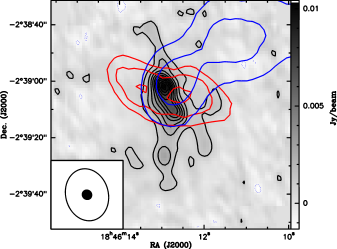
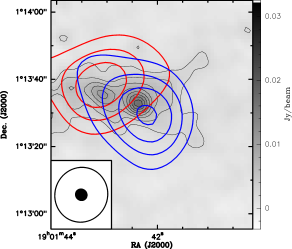
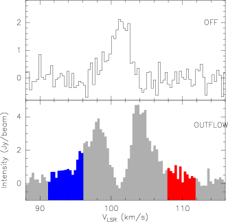
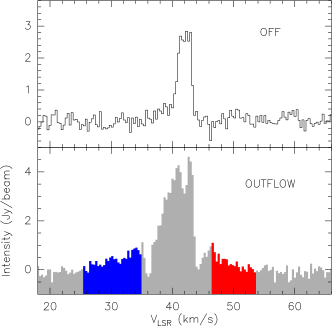
Figure 2: Top Left: G29.96e PdBI 3.5 mm continuum plotted in gray-scales with $\mathrm{HCO^{+}}$ outflow overlaid in contours. Blue (red) contours represent the blueshifted (redshifted) shifted emission between velocities (LSR) of 91 – 96 $\mathrm{km\,s^{-1}}$(108 – 112 $\mathrm{km\,s^{-1}}$.) Top Right: G35.20w PdBI 3.5 mm continuum plotted in gray-scales with $\mathrm{HCO^{+}}$ outflow overlaid in contours. Blue (red) contours represent the blueshifted (redshifted) shifted emission between velocities (LSR) of 25.5 – 35.0 $\mathrm{km\,s^{-1}}$(46.6 – 53.6 $\mathrm{km\,s^{-1}}$.) Bottom Panels: The $\mathrm{HCO^{+}}$ spectra towards the brightest mm position mm1 (i.e. outflow source) and an OFF position for the respective sources in the top panel. The BIMA and PdBI beams are shown in white and black respectively.

The same argument holds for Spitzer data, where we detect protostars at 24 $\mu$m towards the center cores in both filaments (see Figure 4). Similarly, the detection of relatively bright $24\leavevmode\nobreak\ \rm\mu m$ sources in the target clouds suggests the presence of massive luminous stars. In G29.96e, an aperture of $10\arcsec$ radius to measure a flux density of $0.13\leavevmode\nobreak\ \rm Jy$; we subtract backgrounds, which are measured in an annulus inner and outer radii of $10\arcsec$ to $13\arcsec$, respectively. For G35.20w, radii of $13\arcsec$ and $20\arcsec$ are used to derive $2.0\leavevmode\nobreak\ \rm Jy$. In both cases, an aperture correction of 1.167 is used to boost the flux densities. Given extended backgrounds, the measurements suffer from significant uncertainties. These observations can be compared to the luminosity-dependent $24\leavevmode\nobreak\ \rm\mu m$ model flux densities of Dunham et al. (2008), see Parsons et al. (2009) for details. We assume a $24\leavevmode\nobreak\ \rm\mu m$ foreground extinction corresponding to $10^{23}\leavevmode\nobreak\ \rm cm^{-2}$, as suggested by the peak column densities of our target clouds; much lower luminosities apply otherwise. In this framework, the observed flux densities imply luminosities of $6.8\times 10^{3}\,L_{\sun}$ (G29.96e) and $1.5\times 10^{4}\,L_{\sun}$ (G35.20w). This is in the range of luminosities expected for massive young accreting stars (Sridharan et al., 2002).

Finally, Class II methanol masers at 6.7 GHz are detected towards one of the targets (i.e., G29.96e; Sect.3.2.1). These masers are exclusive signposts of the earliest stages of high-mass star formation (Pestalozzi et al., 2007).

4.2 Line widths

A fit to the resolved hyperfine structure of $\mathrm{NH_{2}D}$ allows for an accurate estimate of the line width corrected for any optical depth effects. The observed line width is the sum of the thermal and turbulent components, i.e. FWHM width $\Delta v$, is given by $\Delta v^{2}=\Delta v_{\rm th}^{2}+\Delta v_{\rm nt}^{2}$. For gas temperatures $<20$ K, $\Delta v_{\rm th}<0.22$ $\mathrm{km\,s^{-1}}$. The observed line width, $\Delta v$, is in the range of 0.68 – 1.42 $\mathrm{km\,s^{-1}}$for G29.96e, and 0.5 – 1.69 $\mathrm{km\,s^{-1}}$for G35.20w. The mean and median line width representative of this sample is $\lesssim 1\leavevmode\nobreak\ \rm km\,s^{-1}$. Therefore, the line width is only mildly supersonic ($\Delta v_{\rm nt}/\Delta v_{\rm th}\sim 4$) unlike usually those expected from high-mass star-forming regions McKee & Tan (2002). Recent high resolution observations by Olmi et al. (2010) have also reported such low line widths in massive dense cores. This line width is also smaller than the single dish line width measurements reported towards high-mass IRDCs (for e.g. Pillai et al. 2006a, Pillai et al. 2007). Therefore, we are able (to some extent) resolve the velocity dispersion within the beam, and we can ascertain that the high-mass precluster cores are not necessarily characterized by large velocity dispersions ($>1$ $\mathrm{km\,s^{-1}}$). The implication of this property on the core stability and current theories on high-mass star formation will be discussed in Sect. 5.

4.3 Deuteration: NH₂D vs. NH₃ and dust

The importance of deuteration in our target clouds can be assessed by deriving relative $\mathrm{NH_{2}D}$-to-$\mathrm{NH_{3}}$ abundances, $[{\rm NH_{2}D}/{\rm NH_{3}}]$. These are given in Table 5, calculated using the scheme described in Sect. 3.1.3. Towards the positions with a signal strong enough to permit a reliable abundance measurement, we derive $[{\rm NH_{2}D}/{\rm NH_{3}}]>6\%$. As an average, we find $\langle[{\rm NH_{2}D}/{\rm NH_{3}}]\rangle=15\%$. The maximum relative abundance is $37\%\pm 11\%$. This is high compared to the values reported in literature, for e.g. $[{\rm N_{2}D^{+}}/{\rm N_{2}H^{+}}]$, observed in low mass and intermediate mass prestellar cores (Crapsi et al. 2005, Fontani et al. 2008) as well as $[{\rm NH_{2}D}/{\rm NH_{3}}]$ ratios observed in low mass cores (Crapsi et al. 2007). More recently, Busquet et al. 2010 have reported high deuteration ratios (0.1–0.8) in cores with no associated young stellar objects in a high-mass star-forming region.

Beyond the value of this abundance ratio, it is interesting to see how the abundance of $\mathrm{NH_{2}D}$ varies across the clouds studied here. Because of its particular formation chemistry, $\mathrm{NH_{2}D}$ can effectively be used as a tracer of certain physical conditions. The remainder of this section is dedicated to such studies.

4.3.1 $\mathrm{NH_{2}D}$  chemistry

Let us first examine how deuterated Ammonia — i.e. $\mathrm{NH_{2}D}$ — is supposedly produced. Two aspects warrant particular attention. First, as laid out in Pillai et al. (2007), the deuterium fractionation initiates with the formation of $\mathrm{H_{2}D^{+}}$ through a reaction that plays a role only at low temperatures ($\lesssim 20\leavevmode\nobreak\ \rm K$). The enhanced $\mathrm{H_{2}D^{+}}$ fractionation is then transferred to other molecules including $\mathrm{NH_{3}}$. Second, CO depletion by freeze-out onto dust grains (Tafalla et al., 2002) aids the formation of $\mathrm{NH_{2}D}$, since gas-phase CO “destroys” $\mathrm{H_{2}D^{+}}$  and therefore $\mathrm{NH_{2}D}$ (Caselli et al., 2008). In addition, $\mathrm{NH_{3}}$ does not deplete considerably relative to other molecules. Given similar volatility of the N₂ (parent molecule for $\mathrm{NH_{3}}$ and $\mathrm{NH_{2}D}$) and CO, it is yet unclear why. The deuterium fractionation however is sensitive to temperature such that at temperatures higher than 20  K (close to protostars), release of CO to gas phase together with lower fractionation would lead to a decrease in the $\mathrm{NH_{2}D}$ deuteration. In summary, $\mathrm{NH_{2}D}$ is thus expected to be abundant in cold regions with significant CO depletion.

4.3.2 Spatial abundance patterns

Dust emission and infrared extinction are good probes of $\rm H_{2}$ column density. The coldest cloud regions, and the regions with strongest CO depletion,are usually strongly correlated with $\rm H_{2}$ column density. Therefore, a basic prediction of the formation theory of deuterated analogues of dense gas tracers like $\mathrm{N_{2}H^{+}}$  and $\mathrm{NH_{3}}$ is that they should correlate well with dust emission intensity and extinction features. As seen in Figs.3, this is, in a global sense, the case in G29.96e and G35.20w. There are, however, some interesting exceptions to this general trend.

When examining the correlation of emission from dust, $\mathrm{NH_{3}}$, and $\mathrm{NH_{2}D}$ in more detail we see in Fig.1 that the velocity-integrated $\mathrm{NH_{3}}$ emission correlates very well with the PdBI dust emission map at 3.5 mm (the map at 1.3 mm wavelength is not useful for this because of spatial filtering). This correlation holds in terms of spatial distribution (i.e., dust and $\mathrm{NH_{3}}$ are present in the same regions), as well as in terms of intensity (i.e., very bright regions in dust are also bright in $\mathrm{NH_{3}}$, and vice versa). This situation is entirely different for $\mathrm{NH_{2}D}$; the dust emission peak is not the brightest $\mathrm{NH_{2}D}$ peak in both filaments, thus the brightest dust emission locations do not dominate the $\mathrm{NH_{2}D}$ maps. To give an example, the $\mathrm{NH_{2}D}$-identified P1 position in G29.96e is free of PdBI 3.5 mm dust emission, while P2 coincides with the mm1 dust emission peak; still, both positions are similar in $\mathrm{NH_{2}D}$ brightness. Also, many major $\mathrm{NH_{2}D}$ peak locations (e.g., P1, P2–P4, and P8 in G35.20w) are not unusually bright in 3.5 mm dust emission; sometimes (e.g., P1 in G29.96e), no dust emission at all is detected. Correspondingly (because dust and $\mathrm{NH_{3}}$ have a similar distribution), the detailed correlation of $\mathrm{NH_{2}D}$ and $\mathrm{NH_{3}}$ is not perfect.

To understand these trends, first consider the dust emission peak positions. These are heated by the embedded forming stars; $\mathrm{NH_{3}}$ observations (Table 4) yield gas temperatures $\approx 22\leavevmode\nobreak\ \rm K$ for the mm1 positions in G29.96e and G35.20w. As discussed in Sect. 4.3.1, at these temperatures, deuterium fractionation is expected to drop. Also, the heating can lead to evaporation of CO from dust grains, which will further reduce the $\mathrm{NH_{2}D}$ abundance. The dust emission peaks are thus actually not expected to be particularly rich in $\mathrm{NH_{2}D}$, in case they contain stars (Emprechtinger et al., 2009). The PdBI $\mathrm{NH_{2}D}$ peak intensity map overlaid on the Spitzer 24$\mu$m image in Fig.4 shows a clear offset in the peak position towards the protostar seen in emission at 24$\mu$m in both filaments.

Next, we consider the case of the relatively faint ($\lesssim 9\sigma$) $\mathrm{NH_{2}D}$ peak positions free of detected dust emission. Towards those positions, dark extinction features in the 8 and $24\leavevmode\nobreak\ \rm\mu m$ Spitzer images indicate significant dust column densities. However, the dust emission sensitivities reported in Table LABEL:tab:beam_rms imply $1\leavevmode\nobreak\ \sigma$ column density detection thresholds $\sim 5\times 10^{22}$ $\hbox{{\rm cm}}^{-2}$ for a temperature of 15 K. Thus, it is not surprising that the dust emission towards relatively faint $\mathrm{NH_{2}D}$ cores goes undetected. In fact, a recent 450$\mu$m image of G35.20w taken as part of SCUBA-2 commissioning clearly show the $\mathrm{NH_{2}D}$ streamers that go undetected with PdBI dust continuum (Jenness et al., 2010). Similarly, For G29.96e, the filamentary structure observed in $\mathrm{NH_{2}D}$ coincide with the dark Spitzer extinction features. In summary, the spatial trends observed in $\mathrm{NH_{2}D}$ emission are thus in broad agreement with the theoretical picture drawn in Sect. 4.3.1.

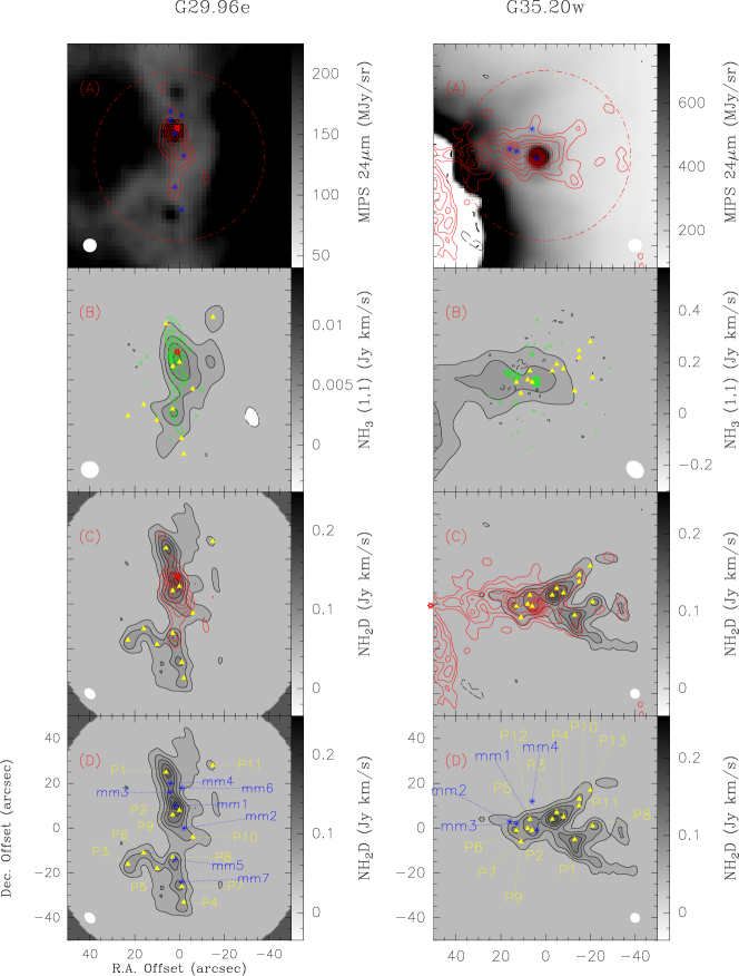
Figure 3: Line and Continuum emission towards G29.96e (left) and G35.20w (right). Panel (A): Spitzer 8$\mu$ (for G29.96e)/24$\mu$ (for G35.20w) emission and 3.5 mm PdBI dust continuum emission as contours. Panel (B): VLA $\mathrm{NH_{3}}$ (1,1) integrated intensity map and 1.3 mm PdBI dust continuum emission as contours. Panel (C): PdBI $\mathrm{NH_{2}D}$ integrated intensity map and 3.5 mm PdBI dust continuum emission as contours. Panel (D): PdBI $\mathrm{NH_{2}D}$ integrated intensity map with the clumps identified from CLUMPFIND from P1. The PdBI primary beam at 3.5 mm is shown as dashed circle in the top most panel. The contour levels for all the maps (line and continuum) start at $-3\sigma$, $3\sigma$ in steps of 3$\sigma$. The positions of the $\mathrm{NH_{2}D}$ cores (P1..) given in Table 4 are marked as filled triangles, the 1.3mm cores (mm1..) are marked as stars and the synthesized beam of the background image shown as filled white ellipses. For G29.96e, we have also marked the methanol maser positions identified by Walsh et al. (1998) as red stars.

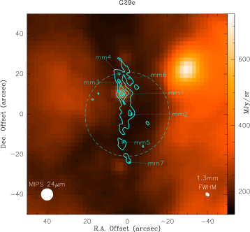
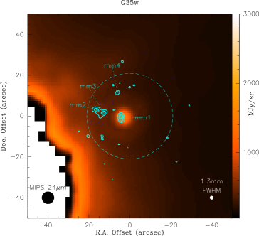
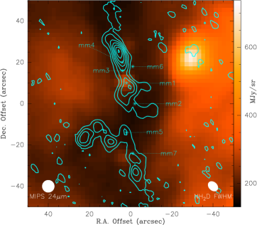
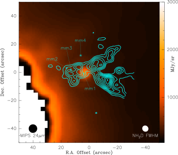
Figure 4: Top Panels: Spitzer 24$\mu$m map (color scale), and PdBI 1.3 mm emission intensity map with the PdBI 1.3 mm primary beam indicated as dashed circle. The contour levels start at $-3\sigma$, $3\sigma$ in steps of 5$\sigma$. Center Panels: Spitzer 24$\mu$m map (color scale), and PdBI $\mathrm{NH_{2}D}$ peak intensity map. The $\mathrm{NH_{2}D}$ contour levels start at $-3\sigma$, $3\sigma$ in steps of 2$\sigma$. Bottom Panels: The $\mathrm{NH_{2}D}$ spectra towards the brightest position for the respective sources in the top panel. The brightest $\mathrm{NH_{2}D}$ peak is is clearly offset from the Spitzer point source and brightest mm core in both cases, and that the clumps are detected at high S/N through out the map.

4.4 Mass estimates

We derive the gas mass from the 1.3 mm and 3.5 mm dust continuum emission as detailed in Sect. 3.1.4). In principle these masses, which were obtained from the flux integrated over a certain area might be influenced by foreground and background emission along the line of sight to the observer. Estimates for density gradients typical of clouds (Kauffmann et al., in prep.) suggest that the mass of embedded cores is usually overestimated by up to a factor 2. However, in our maps, any large scale information is lost in the 1.3 mm data because structures larger than $\approx 19$″ are effectively filtered out by the interferometer. In practice, both biases cancel each other to some extent, and the derived masses and densities are likely to be correct within a factor $\sim{}2$ (when setting uncertainties due to opacities and temperatures aside).

We can quantify the extent of missing flux by comparing the total mass within an aperture for SCUBA and PdBI continuum data. For an aperture with a diameter of 38 ″, which corresponds to the greatest extent of the N-S structure seen in SCUBA data for G29.96e, we estimate the total mass within the filaments to be $2300\,M_{\sun}$ (G29.96e), and $1050\,M_{\sun}$ (G35.20w) from the 3.5 mm data. The single-dish SCUBA continuum mass is derived to be $3550\,M_{\sun}$ (G29.96e), and $2250\,M_{\sun}$ (G35.20w). Therefore, we conclude that the observations suffer from 50 – 65% missing flux on the shortest baselines of the interferometer at 3.5 mm. For G35.20w SCUBA measurements, we used archival SCUBA data because of significant artifacts in our data.

We can also compare the masses derived from the 1.3mm and 3.5mm data. In G29.96e, clumps of masses $\sim 200\leavevmode\nobreak\ {\rm to}\leavevmode\nobreak\ 1000\,M_{\sun}$ are identified in the 3.5 mm dust continuum images. Our 1.3 mm observations, however, reveal twice as many clumps as have been identified at 3.5 mm. This might be because G29.96e is at a distance of 7.4 kpc, so that substructure is easily confused in the 3.5 mm beam. As shown in Table 6, the total mass in 1.3 mm clumps of G29.96e exceeds the total mass in 3.5 mm clumps by a factor 1.3. In G35.20w, however, this ratio is 0.1;g much lesser mass is detected at 1.3 mm, probably because of filtering. This may not be surprising, given that G35.20w is closer by a factor 2.

Virial masses, derived from the $\mathrm{NH_{2}D}$ data, provide an independent mass estimate. Following the framework of Bertoldi & McKee (1992), we define the virial mass as

$$M_{\rm vir}=\frac{5\sigma^{2}R}{G}\,,$$ (1)

where $\sigma$ is the 1-dimensional velocity dispersion, $R$ is the radius of the clump, and $G$ is the constant of gravity. The velocity dispersion is calculated as $\sigma^{2}=\sigma_{\rm th}^{2}+\sigma_{\rm nt}^{2}$, to include thermal and non-thermal contributions to the supporting motions (Sect. 4.6). Velocity dispersions, $\sigma$, derive from FWHM widths, $\Delta v$, as $\sigma=(8\ln[2])^{-1/2}\,\Delta v$. We stress that $M_{\rm{}vir}$ is a characteristic property of a cloud, but is not a strict estimator of the actual mass. Indeed, virial and dust masses can be compared using the virial parameter,

$$\alpha=\frac{M_{\rm vir}}{M}=\frac{{5}{\sigma^{2}}{R}}{GM}\,.$$ (2)

As we see in Table 6 (and discussed further below in Sect. 5.1), $\alpha\ll 1$ for all cores which means that these cores are gravitationally over-bound. The virial masses do thus provide a lower limit to the estimated dust masses. We provide the temperature, size (after deconvolution), column density, volume density, mass, virial parameter, and aperture mass of the identified clumps in Table. 6.

4.5 Correlations between mass and temperature

As discussed in Sect.4.3.2, the brightest dust cores are not the brightest in $\mathrm{NH_{2}D}$. Are these bright dust continuum cores (see Table 6) exceptional? Figure 5 explores the relation between the $\mathrm{NH_{3}}$-derived gas temperatures and the dense core masses (from PdBI dust continuum observations) for these cores. To remove biases due to different source distances, the masses are all calculated for an aperture of 37000 AU diameter. Here, 37000 AU corresponds to the PdBI 3.5 mm beam of $\sim$ 5 arcsec for the more distant source G29.96e.

As we see, the maximum core mass that we derive increases with increasing gas temperature; cores of low mass, for example (i.e., $\leq 40\,M_{\sun}$) are found in all temperature domains, but all massive cores (i.e, $\geq 150\,M_{\sun}$) have high temperatures (i.e., $\geq 18\leavevmode\nobreak\ \rm K$). Most likely, the heating needed to raise the temperatures comes from heating by embedded stars. Heating to temperatures $\gtrsim 10\,K$ can be provided by either (i) a single star luminous (and thus massive) enough to provide the heating, or (ii) a cluster of low-mass stars that is populous enough to have a high luminosity. The luminosity required for the heating is not high; following Eqs. (5, 8) of Kauffmann et al. (2008), $100\,L_{\sun}$ are, e.g., enough to raise the mean dust temperature within a 37000 AU diameter aperture to 20 K.

Regardless of the nature of the sources might be, the dearth of cold (e.g., $\leq 15\leavevmode\nobreak\ \rm K$) high-mass cores ($\geq 100\,M_{\sun}$) suggests that all cores of such high-mass might form stars. These are not entirely devoid of stars and do not exactly represent the conditions before the onset of active star formation. Rather, it is the bright $\mathrm{NH_{2}D}$ cores that are on average colder which represent the initial conditions of high-mass star formation.

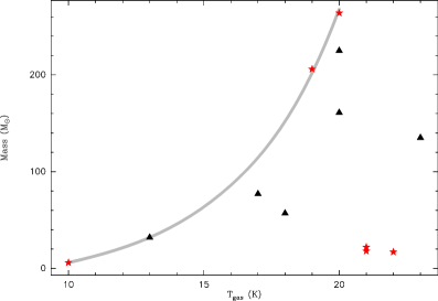
Figure 5: Gas temperature derived from VLA $\mathrm{NH_{3}}$ observations versus the dust mass for the two filaments. Triangles and stars mark G29.96e and G35.20w respectively. The gray curve is shown to indicate the parameter space avoided in mass-temperature space.

4.6 Fragmentation

When trying to understand the initial conditions of (high-mass) star-formation, cloud fragmentation is one of the most important properties to be studied (Field et al., 2008). Indeed, our interferometer observations show that each SCUBA clump fragments into several cores. The initial mass function, star formation efficiency, and star formation rate all depend on cloud fragmentation. To this end, we looked at the fragmentation in our sample from the core separation and their masses (Fig.6).

4.6.1 Theory

This data on cloud fragmentation can be directly compared to predictions from Jeans-type cloud fragmentation (Kippenhahn & Weigert (1990); their Sect. 26.3). In this model, an initially homogeneous state of given characteristic $\rm H_{2}$ particle density and velocity dispersion, $n_{\rm char}$ and $\sigma_{\rm char}$, will fragment into features of mass

$$M_{\rm J}=\varrho\,\ell_{\rm J}^{3}=1.578\,M_{\sun}\,\left(\frac{\sigma_{\rm char}}{0.188\leavevmode\nobreak\ \rm km\,s^{-1}}\right)^{3}\,\left(\frac{n_{\rm char}}{10^{5}\leavevmode\nobreak\ \rm cm^{-3}}\right)^{-1/2}\,,$$ (3)

which are separated by a distance

$$\ell_{\rm J}=\left(\frac{\pi}{G\varrho}\right)^{1/2}\,\sigma_{\rm char}=0.06\leavevmode\nobreak\ {\rm pc}\,\left(\frac{\sigma_{\rm char}}{0.188\leavevmode\nobreak\ \rm km\,s^{-1}}\right)\,\left(\frac{n_{\rm char}}{10^{5}\leavevmode\nobreak\ \rm cm^{-3}}\right)^{-1/2}$$ (4)

($\varrho$ is the mass density implied by $n_{\rm char}$). By comparing the observed masses of cores, and separations between them, to the predicted Jeans-values, we can thus assess whether Jeans-type fragmentation governs the structure formation in our target regions. This is shown in Fig. 6.

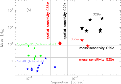
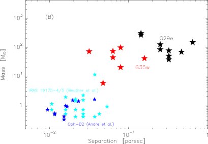
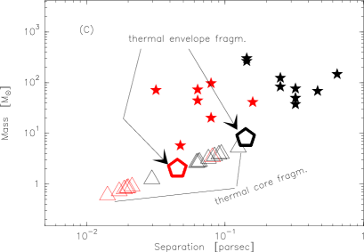
Figure 6: Separation versus core mass. For all panels, stars mark the observations, pentagons mark the envelope properties for thermal/turbulent Jeans fragmentation while triangles mark the core properties. Panel (A): We used 1.3 mm PdBI data for G35.20w(red) and G29.96e(black). The mass sensitivity corresponds to a 3 $\sigma$ rms noise in the final 1.3 mm continuum map for a temperature of 20 K. Data for a high-mass CygnusX-N53 (Bontemps et al., 2010) and low mass protocluster Oph-B2 (André et al., 2007) is shown for comparison. The masses are derived from dust continuum for all the cores. Panel (B): virial mass (scaled by mean virial parameter 0.3) derived from $\mathrm{NH_{2}D}$ data versus separation. Data from two low mass clumps, Oph-B2 (André et al., 2007), and IRAS 19175-4/5 (Beuther & Henning, 2009) is also shown for comparison. The masses correspond to virial masses derived from $\rm N_{2}H^{+}$ 1–0 observations. Panel (C): Same as panel B with the corresponding thermal Jeans mass and length for the respective core density, and temperatures. Panel (D): Same as panel B with the corresponding turbulent Jeans mass and length for the respective core density, and line width.

The densities and velocity dispersions substituted in Eqs. (3, 4) have to be chosen carefully. For a given core, the density will lie between the one of the actual dense core, and the one of the SCUBA-detected envelope. To bracket the reasonable parameter range, we adopt either $n_{\rm char}\to n_{\rm core}$ or $n_{\rm char}\to n_{\rm env}$ in the calculations below. We derive the envelope and core densities from SCUBA 850 $\mu$m and PdBI data respectively as, $n_{\rm char}=\frac{\rm Mass}{\frac{4}{3}\,\pi\,{\rm radius}^{3}}$. Similarly, we use either the thermal velocity dispersion of the mean free particle, $\sigma_{\rm char}\to\sigma_{\rm th}^{\rm mean}$ (using a mean molecular weight of 2.33; Kauffmann et al. 2008), or we also include the impact of non-thermal motions, $\sigma_{\rm char}\to[(\sigma_{\rm th}^{\rm mean})^{2}+(\sigma_{\rm nt})^{2}]^{1/2}$. Depending on whether the core or envelope density is used, we adjust the non-thermal velocity dispersion, $\sigma_{\rm nt}$, to the value for the core or its envelope.

4.6.2 Analysis

Fragmentation is best studied at the highest possible resolution. Here, we rely on our 1.3 mm PdBI maps. Ideally, we would base our analysis on dust emission data, which provides a fairly reliable probe of mass reservoirs. This is shown in panel A of Fig. 6. However, only few cores are detected in dust emission at 1.3 mm wavelength. Therefore, we use the separations and virial masses of $\mathrm{NH_{2}D}$ cores in the following. Here, core separation is defined as the distance to the nearest neighbor as seen in projection on the sky. Since we find that virial masses are always much smaller than the dust masses, we scaled the virial mass by the mean virial parameter (0.3) to reflect the actual core masses. They are presented in Fig. 6B. To guide the reader through the following discussion, the mean observed core size, mass, and density is given by R${}_{\rm eff}=0.14(0.04)$ parsecs, $n_{\rm core}=1.3(8.3)\times 10^{5}$ $\mathrm{cm^{-3}}$  and M${}_{\rm vir}=110(33)$ $\hbox{M}_{\odot}$ for G29.96e(G35.20w).

First consider the case of thermal fragmentation at envelope density ($n_{\rm char}\to n_{\rm env}$, $\sigma_{\rm char}\to\sigma_{\rm th}^{\rm mean}$), indicated by pentagons in panel C of Fig. 6. In G29.96e, the predicted mass for this case falls short of observed values by more than a factor 10. In separation, the discrepancy is up to a factor 10. Similar maximum discrepancies are seen in G35.20w. Thus, the structure of G29.96e and G35.20w is not well described by thermal fragmentation of the envelope. A very similar discrepancy prevails even if we assume core densities ($n_{\rm char}\to n_{\rm core}$, $\sigma_{\rm char}\to\sigma_{\rm th}^{\rm mean}$; triangles in Fig. 6C).

Turbulent Jeans fragmentation at envelope density ($n_{\rm char}\to n_{\rm env}$, $\sigma_{\rm char}\to[(\sigma_{\rm th}^{\rm mean})^{2}+(\sigma_{\rm nt}^{\rm env})^{2}]^{1/2}$, pentagons in Fig. 6D) predicts masses and separations that is inconsistent with observations as seen for thermal fragmentation. The observed values are always lower than the model values. Finally, turbulent Jeans fragmentation at core density ($n_{\rm char}\to n_{\rm core}$, $\sigma_{\rm char}\to[(\sigma_{\rm th}^{\rm mean})^{2}+(\sigma_{\rm nt}^{\rm env})^{2}]^{1/2}$; triangles in Fig. 6D) yields masses and separation predictions that are on average within a factor 3 of the observations. Among the models explored here, this is the best fit to the data.

Thus, the observed masses and separations of the cores are best understood if they result from turbulent Jeans fragmentation. An observable predicted by turbulent fragmentation models is that clump separation scales should scale with mass (Padoan & Nordlund, 2002). We also note that gravitational fragmentation models also claim to make a similar prediction (see Sect.5.2 of Bonnell et al. 2007 for a discussion). Interestingly, our observations lie closer to those predicted for core densities. Thus, it seems plausible that fragmentation occurred closer to core than envelope densities and velocity dispersions.

4.6.3 Previous results

Numerous papers have addressed cloud fragmentation over the last decade. Figures 6A and 6B present, for example, data that are representative of low to intermediate to higher mass protoclusters. Oph-B2 is a well studied low mass protocluster region in the Ophiuchus molecular cloud complex with a total mass of $42\,M_{\sun}$ (Motte et al., 1998). $\rm N_{2}H^{+}$ observation imply subsonic to transonic turbulence (André et al., 2007). Beuther & Henning (2009) study the fragmentation of two clumps of low to intermediate mass, IRAS 19175-4 and 5 (combined single-dish mass of $87\,M_{\sun}$). The velocity dispersions are transonic to supersonic in these sources, just as seen in our targets (Sect.4.2). Also the massive clumps mapped by Zhang et al. (2009b) belong to this latter velocity domain. Ideally, one would want to perform a fragmentation study such as ours on entire massive star-forming complexes like Cygnus-X (Motte et al., 2007). Recently, Bontemps et al. (2010) have studied six individual massive dense cores within this complex in dust continuum at high angular resolution. Bontemps et al.  note that the core size, and separation suggest densities much higher than in a turbulence regulated star formation scenario proposed by McKee & Tan (2002). It would be interesting to combine the continuum data with high angular resolution spectral line data and compare the results with our study. Since this information is not yet available, we derived the minimum separation for one of their massive dense cores CygnusX-53. CygnusX-53 was chosen because their 1.3 mm PdBI continuum observations shows the highest fragmentation toward this core. Comparison with our results is shown in Figure 6A. Clearly, for the same spatial scales, a few cores in CygnusX-N53 have an order of magnitude higher mass than in Oph-B2, the low mass protocluster, in agreement with our naive expectation. Whether fragmentation is turbulence regulated is yet to be answered.

Motte et al. (1998) and Beuther & Henning (2009) both conclude that their separation data are consistent with thermal core fragmentation ($n_{\rm char}\to n_{\rm core}$, $\sigma_{\rm char}\to\sigma_{\rm th}^{\rm mean}$). In contrast, Zhang et al. (2009b) find that thermal envelope fragmentation ($n_{\rm char}\to n_{\rm env}$, $\sigma_{\rm char}\to\sigma_{\rm th}^{\rm mean}$) fails to explain their mass and separation observations. They suggest that turbulence, magnetic fields, or both, may influence fragmentation. Thus, our conclusions are more comparable with the observations by Zhang et al. (2009b). This is not necessarily a surprise, given that our study and Zhang et al. (2009b) explore similar regions, while Motte et al. (1998) and Beuther & Henning (2009) study clumps of much lower mass and turbulence.

4.6.4 Fragmentation sequences & cascades

Intriguingly, all of the fragmentation data plotted in Fig. 6 lie along a common sequence, independent of the nature of the region studied. Mass-separation data for clouds forming stars of lower mass fall at the end with small masses and separations, while observations for turbulent regions forming higher mass stars constitute the opposite end of the sequence. Here we lack the space to discuss the nature of this sequence comprehensively; resolution and intensity detection thresholds may well conspire to yield such an apparent correlation. It may be instructive to explore this finding in future studies.

Another result of the fragmentation analysis is that all studies are consistent with fragmentation occurring at densities and velocity dispersion similar to the present-day values for the cores. Most likely, $n_{\rm char}\to n_{\rm core}$ yields good matches because the telescope resolution highlights a particular spatial scale. At that scale, $n_{\rm core}$ is a characteristic density, simply because of the way cores are extracted. Fragmentation probably occurred at a slightly larger spatial scale of slightly lower density. If true, $n_{\rm char}\to n_{\rm core}$ in fragmentation calculations will thus naturally yield a good description for the emission that is just resolved.

This argument only works if fragmentation continuously occurs at any given spatial scale and density (perhaps with a limit at small scales and high densities). For any given resolution, apparently monolithic objects would break up into smaller fragments, if studied with sufficient resolution. We can detect fragmentation down to $\sim$ twice the beam size (0.02pc for G35.20w, or 0.07pc for G29.96e) but any fragmentation on scales smaller than this would go undetected. In this situation, the fragment masses derived here (or in any other study) only presents a snapshot of the fragmentation cascade taken at a particular scale. Then, they bear no obvious relation to the mass of the star eventually forming from the cloud. This only breaks down at the bottom of the cascade, once fragments with a mass $<M_{\rm J}$ are resolved.

Table 6: Cores identified from the 1.3 mm and 3.5 mm continuum emission. Columns are the clump name (for 1.3mm cores only), offset position relative to the map center, peak flux, total flux, the effective radius after deconvolution with the beam of the mm core, total gas mass for a temperature T_kin estimated from $\mathrm{NH_{3}}$ observations, peak ${\rm H_{2}}$ column density, average gas density over R_eff, total mass, virial mass from $\mathrm{NH_{2}D}$ observations, the alpha parameter as defined in Eq.2, and an aperture mass for an aperture size of 37000 AU. 37000 AU corresponds to the beam of the more distant source G29.96e. The aperture mass is underestimated up to a factor 2 when aperture size is very similar to the beam.

Core	core offsets	Speak	Stotal	Reff	Tkin	N${}_{\rm H_{2}}$	$\rho$	Mtotal	Mvir	$\alpha$	Maperture
	arcsec	Jy/beam	Jy	parsecs	(K)	(1023 $\hbox{{\rm cm}}^{-2}$)	(105 $\mathrm{cm^{-3}}$)	$\hbox{M}_{\odot}$	$\hbox{M}_{\odot}$		$\hbox{M}_{\odot}$
						G29.96e-1.3mm
mm1	( 2, 10)	0.052	0.293	0.16	23.	4.	2.	291.	90.	0.3	135.
mm2	(-2, 0)	0.026	0.200	0.17	16.a	4.	2.	320.	55.	0.2	107.
mm3	( 4, 16)	0.024	0.055	0.07	16.a	4.	9.	88.	19.	0.2	90.
mm4	( 4, 20)	0.020	0.051	0.08	16.a	3.	6.	82.	13.	0.2	83.
mm5	( 2, -14)b	0.018	0.054	0.09	18.	2.	4.	74.	–	–	57.
mm6	(-1, 18)c	0.014	0.036	0.07	16.a	2.	6.	58.	–	–	45.
mm7	(-1, -24)	0.012	0.028	0.07	13.	2.	6.	60.	51.	0.8	32.
						G29.96e-3.5mm
	( 2, 10)	0.010	0.026	0.24	20.	5.	2.	836.	110.	0.1	225.
	(-1, 2)	0.007	0.017	0.21	20.	3.	2.	547.	64.	0.1	161.
	( 2, -15)	0.003	0.005	0.14	17.	2.	2.	193.	42.	0.2	77.
						G35.20w-1.3mm
mm1	( 4, -1)	0.044	0.090	0.03	22.	5.	24.	18.	7.	0.4	17.
mm2	(16, 3)	0.030	0.059	0.03	21.	3.	17.	13.	9.	0.7	22.
mm3	(13, 2)b	0.028	0.051	0.03	21.	3.	14.	11.	–	–	18.
mm4	(6, 12))c,d	0.013	0.012	0.01	10.	5.	265.	8.	–	–	6.
						G35.20w-3.5mm
	( 4, -1)	0.017	0.078	0.15	20.	9.	5.	490.	107.	0.2	264.
	(15, 2)	0.011	0.046	0.13	19.	6.	5.	306.	145.	0.5	206.
	(-13, -11)	0.003	0.009	0.08	16.a	2.	5.	78.	8.	0.1	48.
	(-15, 12)	0.003	0.005	0.06	16. a	2.	6.	40.	13.	0.3	32.

Comments: ^a Mass estimates based on an assumed temperature of  16 K, since measured value has a very high error ($>30\%$).

^b $\mathrm{NH_{2}D}$ spectra at these offsets show clearly more than one velocity component. We did not consider these positions because of the following, (i) poor two-component HFS fit in CLASS in one case, (ii) difficulty of associating a particular component to the dust.

^c No $\mathrm{NH_{2}D}$ detection. ^d mm4 is barely resolved with peak emission just above 5$\sigma$. Given the biases in a typical interferometer image, this might be spurious.

5 Models of star formation: stability & accretion

In recent years, two models for the formation of massive stars have proven particularly influential: (i) the monolithic collapse of massive cloud fragments supported by supersonic turbulent pressure (McKee & Tan 2002; essentially like Shu 1977, with scaled-up velocity dispersions); and (ii) rapid growth of many cores of initially very low mass via competitive accretion from a common massive mass reservoir (Zinnecker 1982; Prediction of the protostellar mass spectrum in the Orion near-infrared cluster; Bonnell et al. 2001, 2004, 2007). Some of our data are suited to test the one or the other of these two scenarios.

Beyond this, we derive estimates of various key properties of out target clouds. This includes their stability against collapse, magnetic fields, and rates for mass accretion onto the cores.

5.1 Turbulent and magnetic cloud support

Random motions in excess of the thermal ones can contribute to the support of an object against self-gravity (Bertoldi & McKee, 1992). The impact of such turbulent motions is captured by the virial mass and ratio (Eqs. 1, 2). In these, the adopted velocity dispersions reflect thermal as well as further random motions. A cloud fulfilling the stability criteria of Ebert (1955) and Bonnor (1956), for example, has $\alpha>2.06$ (Bertoldi & McKee, 1992). The exact stability threshold with respect to collapse depends on the nature of the adopted equation of state. For reasonable assumptions, $\alpha\ll 1$ implies a lack of pressure support against collapse, hence subvirial.

As shown in tables 4 and 6, $\alpha\ll 1$ holds for all cores and clumps identified in our target regions. Table 6 gives the $\alpha$ values for dust and virial mass computed from the 3.5 mm PdBI continuum and line ($\mathrm{NH_{2}D}$) data corresponding to the dust cores. The mean (median) $\alpha$ for the cores is 0.3 (0.2). Similarly, the $\mathrm{NH_{2}D}$ cores identified with CLUMPFIND and listed in Table 4 have also a mean alpha of $0.3$. We do the same estimate for the clump scale for G29.96e and G35.20w since we have the SCUBA data. Comparing the virial mass derived based on average line width from $\mathrm{C^{18}O}$ 2–1 IRAM 30m observations to that of the clump mass from SCUBA data for a $\sim$ 38″ aperture around the brightest peak in G29.96e and G35.20w, we estimate alpha to be 0.3 and 0.2 respectively. Here we have used the relatively low density gas $\mathrm{C^{18}O}$ line widths as opposed to $\mathrm{NH_{2}D}$ as $\mathrm{C^{18}O}$ is more representative of envelope properties. We thus conclude that the observed supersonic turbulent motions, in combination with the (negligible) thermal support, are not sufficient to prevent the cores from collapsing.

Our assessment that $\alpha{}\ll{}1$ is robust with respect to observational uncertainties. Equation (2) shows that $\alpha{}\propto{}\sigma^{2}{}R/M$. The uncertainties on the velocity dispersion, $\sigma$, are negligible. The radius, $R$, has no uncertainty, since it is a freely chosen parameter (as long as $\sigma$ and $M$ are measured for the chosen $R$). The mass is — because of our limited knowledge of dust opacities and temperatures — probably uncertain by a factor $\sim{}2$. This implies a similar uncertainty for $\alpha$. Since our typical observation is $\alpha{}\lesssim{}0.3$, this uncertainty still robustly implies $\alpha{}\ll{}1$. Furthermore, the spatial filtering implies actual masses exceeding the observed ones, and thus virial parameters lower than the derived ones. Large distance errors, $\delta{}d$, are needed to yield large errors in $\alpha$: $(\alpha+\delta{}\alpha{})/\alpha=[(d+\delta{}d)/d]^{-1}$. Distance errors larger than a factor 2 are thus needed to significantly affect $\alpha$. This seems unlikely, in particular given the parallax-based result for G35w.

The observation $\alpha\ll 1$ does not imply that the cloud fragments are collapsing. In particular, there might be additional support from magnetic fields, for which we did not account in the above calculation. Following the virial energy argument used in the initial definition of $M_{\rm vir}$ (see Bertoldi & McKee 1992 for details), we can define a magnetic virial mass,

$$M_{B,\rm vir}=\frac{5R}{G}\,\left(\sigma^{2}+\frac{1}{6}\sigma_{\rm A}^{2}\right)\,,$$ (5)

and a magnetic virial ratio,

$$\alpha_{B}=\frac{M_{B,\rm vir}}{M}\,,$$ (6)

where

$$\sigma_{\rm A}=\frac{B}{(\mu_{0}\varrho)^{1/2}}$$ (7)

is the Alfvén velocity for given magnetic field, $B$ (in SI; $\mu_{0}$ is the permeability of free space). This approach captures the basic aspects of magnetic cloud support, and is well-suited to order-of-magnitude estimates. Researchers requiring a higher degree of accuracy, though, may wish to employ more accurate schemes (see Sect. 2.3 of Bertoldi & McKee 1992).

The magnetic field necessary to support the fragments can be estimated from Eqs. (6, 7) by requiring $\alpha_{B}=1$. For the entire clump, we get $670\leavevmode\nobreak\ \rm\mu G$ (G29.96e), and $1650\leavevmode\nobreak\ \rm\mu G$ (G35.20w). For the cores in both filaments, we find that on average $\sim 1\leavevmode\nobreak\ \rm mG$ field is needed to fulfill $\alpha_{B}=1$. Such field strengths may seem high and unrealistic, in light of recent measurements for low mass dense cores. However, observations spanning a large range in densities have revealed a field-density relation, such that $B\propto n^{1/2}$ (Troland & Heiles, 1986; Padoan & Nordlund, 1999; Vlemmings, 2008). With a lot of upper limits, particularly at the cold core densities, this relation has a significant amount of scatter. Even so, it is interesting to note that the limits on magnetic fields derived by us are not grossly inconsistent with the proposed relation. Specifically, our results for field strengths are not inconsistent with the compilation by Padoan & Nordlund (1999), examined at densities $\sim 10^{5}\leavevmode\nobreak\ \rm cm^{-3}$. However, a preliminary analysis of our own Zeeman and polarization observations towards high-mass cores are inconsistent with a high magnetic field, which would be relatively easy to detect (Pillai et al., work in progress).

Our observations of $\alpha\ll 1$ render the McKee & Tan (2002) model quantitatively not applicable to our target clouds. To see this, consider the basic assumptions of their model: cloud fragments are modeled as equilibria supported by turbulent random motions. Our targets do not bear any similarity with such equilibria, though: these would have $\alpha\gtrsim 1$ (e.g., McKee & Tan 2003), while our observations show $\alpha\ll 1$. In detail, our observations do thus not rule out monolithic collapse. However, the quantitative description by McKee & Tan (2002) cannot apply here.

Global infall motions, as suggested by our $\alpha\ll 1$ observations, are a common feature in many models of competitive accretion. In these models, the whole clump undergoes global collapse, and the gas accretion and the protocluster evolution occurs on the global dynamical timescale. Recently, Krumholz et al. (2005) did actually use $\alpha$ to rule out models with competitive accretion. They assert an apparent lack of observational evidence for $\alpha\ll 1$—a gap now filled by our data. In fact, our observations are not the first to suggest a possible global infall. Two recent studies towards low and intermediate mass star forming regions find evidence of such large-scale collapse (André et al. 2007, Peretto et al. 2007). Also, note that a preliminary numerical model by Vázquez-Semadeni et al. (2008) indicates that physical properties in high-mass star-forming regions can be reproduced by starting with such a global infall.

5.2 Accretion rates onto cores and stars

The formation of massive stars inevitably requires high accretion rates, $\dot{M}$. A fundamental constraint is that a star of mass $M_{\star}$ must accrete all of its mass in one accretion time scale, $\tau_{\rm accr}$. Then, $\dot{M}_{\star}^{\rm time}=M_{\star}/\tau_{\rm accr}$, respectively

$$\dot{M}_{\star}^{\rm time}=10^{-4}{M_{\sun}\leavevmode\nobreak\ {\rm yr^{-1}}}\left(\frac{M_{\star}}{10\leavevmode\nobreak\ M_{\sun}}\right)\,\left(\frac{\tau_{\rm accr}}{10^{5}\leavevmode\nobreak\ \rm{yr}}\right)^{-1}\,.$$ (8)

A normalization of $\tau_{\rm accr}$ to $\lesssim 10^{5}\leavevmode\nobreak\ \rm yr$ is implied by several lines of argument. Recent Spitzer surveys of solar neighborhood clouds yield accretion timescales $\sim 5\cdot 10^{5}\leavevmode\nobreak\ \rm yr$ for low-mass stars (Evans et al., 2009). Given the shorter free-fall times for the more massive cores considered here, one may thus expect shorter timescales for massive stars. Furthermore, theoretical models of the collapse of massive dense cores imply durations $\sim 10^{5}\leavevmode\nobreak\ \rm yr$ (McKee & Tan, 2002). Observational constraints from source counts for different evolutionary stages actually imply $3\cdot 10^{4}\leavevmode\nobreak\ \rm yr$ (Motte et al. 2007, Parsons et al. 2009). The duration of the accretion phase thus robustly implies $\dot{M}_{\star}^{\rm time}\gtrsim 10^{-4}{M_{\sun}\leavevmode\nobreak\ {\rm yr^{-1}}}$ for stars more massive than $10\,M_{\odot}$.

A particular constraint for spherical accretion on massive stars results from the “accretion luminosity problem”: the momentum of the accreting matter has to overcome the star’s radiation pressure (Wolfire & Cassinelli, 1987). Following Jijina & Adams (1996), we estimate that a rate exceeding

$$\dot{M}_{\star}^{\rm lumi}=1.2\times 10^{-6}{M_{\odot}\leavevmode\nobreak\ {\rm yr^{-1}}}\left(\frac{M_{\star}}{10\leavevmode\nobreak\ M_{\odot}}\right)^{-1/2}\,\left(\frac{L_{\star}+L_{\rm accr}}{5\cdot 10^{3}\leavevmode\nobreak\ L_{\odot}}\right)^{5/4}$$ (9)

is needed to overcome the radiation pressure. In this, the combined luminosity of star and accretion, $L_{\star}+L_{\rm accr}$, is normalized to regular observed luminosities. Note that $\dot{M}_{\star}^{\rm lumi}<\dot{M}_{\star}^{\rm time}$ for the case considered here. Thus, the accretion luminosity problem does not imply higher rates than required by basic lifetime arguments. Thus, $\dot{M}_{\star}\approx\dot{M}_{\star}^{\rm time}$.

Direct observations of accretion flows in Hii regions actually imply even higher accretion rates $\sim 10^{-3}{M_{\odot}\leavevmode\nobreak\ {\rm yr^{-1}}}$ (Keto & Wood, 2006). This is in line with observations of nearby young high-mass stars (e.g., Cesaroni et al. 2005). It is not clear, though, how representative these values are.

Equations (8, 9) imply high stellar accretion rates (i.e., onto the stellar surface). These rates have to be supplied by the stellar environment, such as the cores identified here. Thus, it is interesting to also consider core accretion rates, i.e., the rates by which cores (or any other environment of a star) gains mass from its surroundings. Both these rates are considered below.

5.2.1 Accretion of mass onto stars

First, let us consider the rate at which mass accretes onto the central star. A very basic accretion model is the monolithic collapse of the entire core of mass $M$ during the free–fall timescale, $\tau_{\rm{}ff}=(3\pi{}/[32G\langle{}\varrho{}\rangle])^{1/2}$ ($G$ is the constant of gravity, and $\langle{}\varrho{}\rangle$ the mean density), so that $\dot{M}_{\star}^{\rm{}ff}=M/\tau_{\rm{}ff}$. In practice, $\tau_{\rm{}ff}=9.8\times{}10^{4}\leavevmode\nobreak\ {\rm{}yr}\,(\langle{}n\rangle{}/10^{5}\leavevmode\nobreak\ {\rm{}cm^{-3}})^{-1/2}$. We find mean free–fall accretion rates of $0.6\times{}10^{-3}\,M_{\sun}\,\rm{}yr^{-1}$ and $3\times{}10^{-3}\,M_{\sun}\,\rm{}yr^{-1}$ for G35.20w and G29.96e, respectively. This is well within the range required for massive star formation.

McKee & Tan (2002, 2003) present a more elaborate model of such a monolithic collapse. As an initial condition, the model chooses an equilibrium core supported by non-thermal pressure described by a velocity dispersion, $\sigma$, and a polytropic exponent $\gamma_{P}$. Then, the core undergoes the classical inside-out collapse, resulting into accretion onto a star forming in the core’s center. Re-evaluation of the McKee & Tan calculations shows that the maximum accretion rate from a configuration that is initially in equilibrium is found for $\gamma_{P}=1.06$,

$$\dot{M}_{\star}^{\rm eq}\leq 2.3\times 10^{-4}\,M_{\sun}\,\left(\frac{\sigma}{\rm km\,s^{-1}}\right)^{3}\,.$$ (10)

Unfortunately, it is not clear what values are to be substituted for $\sigma$. If we use the greatest velocity dispersions, $(8\ln[2])^{-1/2}\,{}\Delta{}v$, resulting from the observations reported in Table 4, then we derive implied accretion rates of up to $0.6\times{}10^{-4}\,M_{\sun}\,\rm{}yr^{-1}$ and $1.1\times{}10^{-4}\,M_{\sun}\,\rm{}yr^{-1}$ for G29.96e and G35.20w, respectively. This is about consistent with the rate of $10^{-4}\,M_{\sun}\,\rm{}yr^{-1}$ implied by Eq. (8). Also, we find these high rates primarily towards the dust emission peaks where massive stars are observed to form. But this also suggests that the velocity dispersions are increased by stellar feedback and are not representative of the initial conditions to be substituted in Eq. (10).

On average, the observations in Table 4 imply $\langle{}\dot{M}_{\star}\rangle{}\leq{}3\times{}10^{-5}\,M_{\sun}\,\rm{}yr^{-1}$. If representative of the initial state, this is too low for massive star formation. Also, recall that $\alpha{}\ll{}1$, which renders the McKee & Tan (2002, 2003) model not applicable. This observation does, however, not challenge general models of monolithic collapse, which may well obey other accretion laws than explored here.

5.2.2 Accretion of mass onto cores

We may also consider the mass evolution of the reservoir (the “core”) from which a star forms. In our study, this reservoir does probably about correspond to the cores extracted from the interferometer maps. It depletes in mass via accretion onto the star. But the reservoir may also gain mass by accretion onto itself. Here, we derive a new idealized model for this process.

A very basic model of accretion onto cores can be established when idealizing a core as a sphere with radius $R$ that coasts at speed $v$ through a medium of density $\varrho$ and velocity dispersion $\sigma_{\rm{}env}$. Provided collisions with this sphere are inelastic, the sphere-environment collisions due to the sphere’s motion, as well as the drift of gas particles towards the sphere due to random motion, will collect mass at a rate

$$\dot{M}_{\rm{}core}=\pi R^{2}\varrho\left[\sigma+\frac{\pi}{2}v+\int_{0}^{1/2}\left|\sigma-v\,\cos(\vartheta)\right|\,\sin(\vartheta)\,{\rm{}d}\vartheta\right]\,.$$ (11)

This equation can be derived by separately considering the gas particles facing the “front side” and the “back side” of the moving sphere. On the front side, for the first half of particles with random motion towards the core, the mean core–gas relative velocity is $v_{\rm{}rel}=v\,{}\cos(\vartheta)+\sigma$. For the other half, $v_{\rm{}rel}=v\,{}\cos(\vartheta)-\sigma$, where $\vartheta$ is the position angle of a particle with respect to the core’s direction of motion. Similar relations hold for the gas on the back side. At every position on the sphere, mass contained in one of the four populations of gas particles (i.e., two gas motion directions per hemisphere) hits the surface at a rate ${\rm{}d}\dot{M}_{\rm{}core}=(\varrho/2)\,v_{\rm{}rel}\,{\rm{}d}A$, as long as $v_{\rm{}rel}>0$ for the gas population considered. In this, ${\rm{}d}A=2\pi{}R^{2}\,\sin(\vartheta)\,{\rm{}d}\vartheta$ is the surface element. Summation over the populations, and integration over all angles where $v_{\rm{}rel}>0$, then yields Eq. (11).

It is convenient to examine two extreme cases, in which Eq. (11) assumes are more simple form. First, let us consider the case of cores moving through their environment at a very high speed, $v\gg{}\sigma$. Then, the rate at which the core accretes mass that “flies by” becomes $\varrho{}Av$, or

$$\dot{M}_{\rm core}^{\rm{}fly-by} = 2.2\times 10^{-5}\,M_{\sun}\,{\rm yr}^{-1}\,$$ (12)

$$\quad\quad\left(\frac{n}{10^{4}\leavevmode\nobreak\ \rm cm^{-3}}\right)\,\left(\frac{v}{\rm km\,s^{-1}}\right)\,\left(\frac{R}{0.1\leavevmode\nobreak\ \rm pc}\right)^{2}\,,$$

where $A$ is the cross section. To estimate the relative core-envelope motion, we may assume that the ensemble of cores rests with respect to the environment. Then, the dispersion of the core-core relative motions, $\sigma_{\rm core-core}$, gives the mean core-environment relative motion along the line of sight. In 3-dimension, the relative motion is larger by a factor $3^{1/2}$, i.e. $v=3^{1/2}\times\sigma_{\rm core-core}$. Table 7 presents some rate estimates calculated for these assumptions. The environmental density is estimated based on SCUBA data (estimate from Curran et al. 2004 for G35.20w). The G29.96e is broken up into several parts, to reflect the variety of cloud conditions in this region. We find fly-by accretion rates in the range $0.4\leavevmode\nobreak\ {\rm to}\leavevmode\nobreak\ 5\times 10^{-4}\,M_{\sun}\leavevmode\nobreak\ \rm yr^{-1}$.

Second, let us explore the situation of vanishing core-environment motion, $v\ll{}\sigma$. This “turbulent” accretion is only due to random motion of particles towards the sphere. The rate becomes $\varrho{}A\sigma_{\rm{}env}/2$, in which $A$ is the core’s surface, or

$$\dot{M}_{\rm core}^{\rm{}turb} = 4.4\times 10^{-5}\,M_{\sun}\,{\rm yr}^{-1}\,$$ (13)

$$\quad\quad\left(\frac{n}{10^{4}\leavevmode\nobreak\ \rm cm^{-3}}\right)\,\left(\frac{\sigma_{\rm{}env}}{\rm km\,s^{-1}}\right)\,\left(\frac{R}{0.1\leavevmode\nobreak\ \rm pc}\right)^{2}\,.$$

We gauge $\sigma_{\rm{}env}$ by setting it equal to the velocity dispersion in the $\rm{}C^{18}O$ 2–1 transition, as observed with the IRAM 30m–telescope towards the phase center of the PdBI map. Values are given in Table 7. Rates $\geq{}3\times{}10^{-4}$ $\hbox{M}_{\odot}$ are found.

Table 7: Core accretion rates. The columns are, (i) the region of the filament, (ii) number of cores for that region, (iii) mean radius of the cores, (iv) mean velocity dispersion from PdBI $\mathrm{NH_{2}D}$  (v) mean $\rm{}C^{18}O$ envelope velocity dispersion, (vi) mean protocluster density (SCUBA 850$\mu$m), (vii) mean fly–by accretion rate, and (viii) mean turbulent accretion rate.

Source	$N_{\rm cores}$	$R$	$\sigma_{\rm core-core}$	$\sigma_{\rm{}env}$	$n$	$\langle\dot{M}_{\rm core}^{\rm{}fly-by}\rangle$	$\langle\dot{M}_{\rm core}^{\rm{}turb}\rangle$
		pc	$\mathrm{km\,s^{-1}}$	$\mathrm{km\,s^{-1}}$	$10^{4}$ $\mathrm{cm^{-3}}$	$10^{-4}$ $\hbox{M}_{\odot}$$\rm yr^{-1}$	$10^{-4}$ $\hbox{M}_{\odot}$$\rm yr^{-1}$
G29.96e
North filament	4	0.22	0.5	1.4	5	4.6	14.5
South filament	3	0.15	0.2	1.4	2.5	0.4	3.4
G35.20w
Whole filament	13	0.06	0.5	1.1	30	2.3	5.2

This model of core accretion is very simplistic; for example, if collisions were truly inelastic, the inhibition of rebound after particle collisions would imply the strict absence of kinetic pressure. Still, our toy model shows that a dense core is in steady contact with a large mass reservoir, from which it could at least in principle collect mass at a significant rate.

Thus, the accretion rate onto the core might be similar to the accretion rate onto the massive stars, i.e. $\dot{M}_{\rm core}\sim\dot{M}_{\star}^{\rm time}$. This means that the mass reservoir from which stars form is not limited to the cores: the core mass received by the star can be replenished by accretion onto the core. In other words, $M_{\star}>M_{\rm core}$ is entirely consistent with the rates. For core identification schemes as adopted here, a direct correlation of core and stellar masses is not implied by our observations. This is similar to models of competitive accretion, where several stars accrete from a common environment, so that their growth is not limited by the mass reservoir immediately surrounding them.

6 Summary

Although there have been many studies at high angular resolution towards evolved high-mass objects (protostars, Hii regions, outflows associated with protostars), those with the right choice of line tracer (that trace the cold prestellar/cluster gas) with high spectral resolution and sensitivity towards precluster gas has been few. We present high angular resolution observations of two cold,and high-mass filaments G29.96e, and G35.20w, in the close vicinity of two well known UCHii regions G29.96-0.02 and W48 respectively. To our knowledge, these are the first observations that look at the massive cold cores with a line tracer that uniquely traces cold, and dense gas ($\mathrm{NH_{2}D}$). G29.96e is an IR dark cloud as seen with Spitzer at 8$\mu$m, while except for the central object, G35.20w is IR quiet at Spitzer 24$\mu$m. The clustered nature of star formation implies that such filaments are ideal laboratories for determining the initial conditions of high-mass star formation.

Our findings are based on observations obtained in line ($\mathrm{NH_{2}D}$  $\mathrm{NH_{3}}$  HCO⁺), and continuum (3.5 mm, and 1.3 mm) with PdBI, VLA, BIMA, SCUBA, and Spitzer. If the properties of the two filaments were to reflect the initial conditions for forming high-mass stars, then we make the following conclusions that have to be taken into consideration in future models of high-mass star formation;

• $\mathrm{NH_{2}D}$ is a good tracer of the entire filament seen in dust emission with single dish, and shows rich structure along both the filaments. Multiple objects were detected in $\mathrm{NH_{2}D}$  as well as $\mathrm{NH_{3}}$. Millimeter dust continuum detected at high S/N were detected only towards few of these objects. Only the brightest mm continuum core shows several signs of high-mass star formation, with their compact 24 $\mu$m emission, high masses, densities, associated massive outflows, and methanol maser emission. Therefore, gas is predominantly precluster.

• The core temperature is always $<22$ K as derived from our $\mathrm{NH_{3}}$ observations.

• High deuteration seen on large scales is also observed on the small scales resolved by the interferometer. Such high deuteration ratios ([$\mathrm{NH_{2}D}$/$\mathrm{NH_{3}}$]$>6\%$), make the discoveries discussed below possible. We find clear evidence of $\mathrm{NH_{2}D}$ being destroyed in cores showing protostellar activity.

• We studied the fragmentation of these cores, and compared them with two local and far away low mass precluster cores. We find that our observations are consistent with turbulent Jeans fragmentation of massive clumps into cores (from a Jeans analysis).

• The observed velocity dispersions towards the precluster cores are low ($<1$ $\mathrm{km\,s^{-1}}$), and therefore are characterized by low level of turbulence.

• The cores as well as clumps are “over-bound/subvirial”, i.e. turbulence is too weak to support them against collapse, meaning that some models of monolithic cloud collapse are quantitatively inconsistent with data.

• Accretion from the core onto a massive star which can (for observed core sizes and velocities) be sustained by “fly-by accretion” of envelope material onto the core, suggesting that (similar to competitive accretion scenarios) the mass reservoir for star formation is not necessarily limited to the natal core.