Anomalous Fisher-like zeros for the canonical partition function of noninteracting fermions

Abstract

Noninteracting fermions, placed in a system with a continuous density of states, may have zeros in the $N$-fermion canonical partition function on the positive real $\beta$ axis (or very close to it), even for a small number of particles. This results in a singular free energy, and instability in other thermal properties of the system. In the context of trapped fermions in a harmonic oscillator, these zeros are shown to be unphysical. Our results are also applicable to mean-field canonical calculations for fermions. By contrast, similar bosonic calculations with continuous density of states yield sensible results.

Statistical mechanics of model systems Quantum statistical mechanics

Long back, Lee and Yang [1, 2] pointed out that the onset of a phase transition could be deduced by studying the zeros of the grand partition function on the complex fugacity plane. As the number of particles goes to infinity in the thermodynamic limit, the complex zeros tend to pinch the real fugacity axis, signalling a phase transition. Later, Fisher [3] found a similar behaviour of the canonical partition function $Z_{N}(\beta)$ on the complex $\beta$ (inverse temperature) plane near a phase transition. Given a single-particle partition function $Z_{1}(\beta)$, $Z_{N}(\beta)$ may be calculated exactly for noninteracting bosons or fermions using recursion relations [4]. The single-particle partition function may arise from a one-body trapping potential, or may be the result of a calculation in a many-body problem. In this context, Mülken et al. [5] have studied the pattern of Fisher zeros for trapped noninteracting bosons in a harmonic oscillator. As the number of bosons was increased, the real positive $\beta$ axis tended to be pinched at $T=T_{c}$, the Bose-Einstein condensation temperature for spatial dimensions $d>1$. The behaviour of the heat capacity as a function of $T$ also showed a sharp peak for large $N$ at $T=T_{c}$. As expected, this was found both for the exact single-particle density of states of a harmonic oscillator (HO), and for the corresponding (asymptotic) continuous density of states. Mülken et al. [5] examined the distribution of zeros on the complex $\beta$ plane to classify the order of the phase transition in finite systems. Similar analyses were done with the Fisher zeros in interacting statistical models by Janke et al. [6, 7].

Noninteracting fermions trapped in a HO have not been studied in this context, presumably because no irregularity or phase transition is expected. However, a classical version of this formalism has been applied in a model for the thermodynamic properties of nuclear multifragmentation in heavy-ion collisions [8]. In this paper, we are especially interested in the effects of the Fermi statistics on the analytical properties of the canonical partition function. In particular, we compare results obtained from the exact single-particle partition function from the discrete HO energy spectrum, with those obtained using a continuous density of states approximation. The latter is widely used in the grand canonical formalism. With the exact HO density of states, the fermionic system shows no evidence of any phase transition in any dimension, as expected. With continuous density of states, however, we obtain some very surprising results, to be described below. We conclude that for fermions trapped in a HO, or, for that matter, confined in a box, these zeros are spurious. We should mention here that in quantum field theory, lattice calculations of free Wilson fermions also manifest a real zero on the analogous inverse coupling axis if periodic boundary conditions are used [9]. This also gives rise to anomalous properties of the system [10]. Our paper may stimulate the search for spurious zeros of the canonical partition function in other areas of physics. They may appear when a continuous density of states is used that relaxes the restrictions in long-range correlations, or the use of improper boundary conditions. The long-range correlations in our case arose from the Pauli principle, but in other cases may conceivably arise from long-range interactions.

The $N$-particle canonical partition function is generated from a one-body partition function $Z_{1}(\beta)$ by using a recursion relation [4]

$$Z_{N}(\beta)=\frac{1}{N}\sum_{k=1}^{N}\sigma^{k+1}Z_{1}(k\beta)Z_{N-k}(\beta)~{},$$ (1)

where $\sigma=1$ for bosons, and $(-1)$ for fermions, and $Z_{0}(\beta)=1$. The particles are (otherwise) taken to be noninteracting and identical, but correlations coming from quantum statistics are included. In this paper, for analytical simplicity, the particles are taken to be noninteracting, and in a $d$-dimensional isotropic harmonic oscillator. The corresponding one-body partition function is given by [11]

$$Z_{1}(\beta)=\left[\sum_{n=0}^{\infty}e^{\textstyle-(n+1/2)\hbar\omega\beta}\right]^{d}=\left[\frac{1}{2\sinh(\hbar\omega\beta/2)}\right]^{d}~{},$$ (2)

where we have not included the spin degeneracy for fermions. This $Z_{1}(\beta)$, when substituted in eq. (1), enables us to calculate $Z_{N}(\beta)$ exactly for noninteracting bosons or fermions occupying the discrete HO spectrum of energies. The single-particle density of states, $g(\epsilon)$ may be obtained from a Laplace inversion of $Z_{1}(\beta)$, and may be written as a sum of a smoothly varying part $\widetilde{g}(\epsilon)$, and an infinite sum of oscillatory terms [11]. For example, for $d=2$, $g^{(2)}(\epsilon)=\Sigma_{n=0}^{\infty}(n+1)\delta(\epsilon-(n+1)\hbar\omega)$, and may be written exactly as

$$g^{(2)}(\epsilon)=\frac{\epsilon}{(\hbar\omega)^{2}}\left[1+2\sum_{k=1}^{\infty}\cos\left(2\pi k\frac{\epsilon}{\hbar\omega}\right)\right].$$ (3)

To see how this comes about, note that [12]

$$Z_{1}(\beta)=\dfrac{1}{4}\mathrm{cosech}^{2}\left(\dfrac{\hbar\omega\beta}{2}\right)=\dfrac{1}{4}\sum_{n=-\infty}^{\infty}\dfrac{1}{\left(\dfrac{\hbar\omega\beta}{2}+in\pi\right)^{2}}~{},$$ (4)

with no restriction on $\beta$. On taking the Laplace inverse with respect to $\epsilon$, the single pole at $\beta=0$ for $n=0$ yields the first term on the right-hand side of eq. (3) , and the two poles for every integer $n>0$ at $\beta=\pm 2in\pi/\hbar\omega$ give rise to the oscillatory terms. The continuous part of the density of states above is $\epsilon/(\hbar\omega)^{2}$, which we denote by $\widetilde{g}^{(2)}(\epsilon)$. In thermodynamic calculations, it is the continuous density of states $\widetilde{g}^{(d)}$ that is used widely. The smooth one-body (Thomas-Fermi) partition function in $d$ dimensions is

$$\widetilde{Z}_{1}(\beta)=\frac{1}{(\hbar\omega\beta)^{d}}~{},$$ (5)

whose Laplace inverse yields the continuous density of states

$$\widetilde{g}^{(d)}(\epsilon)=\dfrac{\epsilon^{d-1}}{(d-1)!(\hbar\omega)^{d}}~{}.$$ (6)

The zeros of $Z_{N}(\beta)$ on the complex $\beta$ plane may be calculated for bosons as well as fermions. Note that the analytical expression for $Z_{N}(\beta)$ is determined by the choice of $Z_{1}(\beta)$ given by eq. (2), or its continuous counterpart $\widetilde{Z_{1}}(\beta)$ defined above. Schmidt and Schnack [14] have expressed $Z_{N}(\beta)$ in terms of polynomials in $\exp(-\hbar\omega\beta)$, which make the calculation of the zeros for the discrete cases manageable. As stated earlier, the bosonic calculations had been done in Ref. [5], and we repeated some of these to check our programs. Our calculations showed a clear tendency, even for as few as $N=10$ bosons, for Fisher zeros to approach the real positive $\beta$ axis for $d=2$, and more so for $d=3$. This is shown in fig. 1

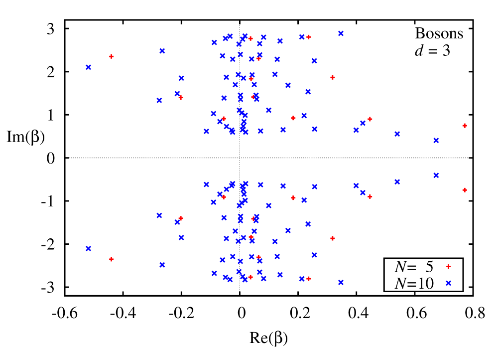
Figure 1: (Color online) The zeros of the exact $Z_{N}(\beta)$, for $N=5$ and $N=10$, obtained from $Z_{1}(\beta)$ of eq. (2) as a function of $\beta=1/kT$ for noninteracting bosons in a three-dimensional harmonic oscillator well.

Although the actual distribution of zeros on the complex plane differed for the discrete and the continuous density of states, both showed the expected behaviour as $N$ was increased. These bosonic results have been studied [5], and will not be displayed further.

We now present the fermionic results. Consider first the discrete density of states, which gives rise to $Z_{1}(\beta)$ of eq. (2), and the resulting $Z_{N}$ for fermions.

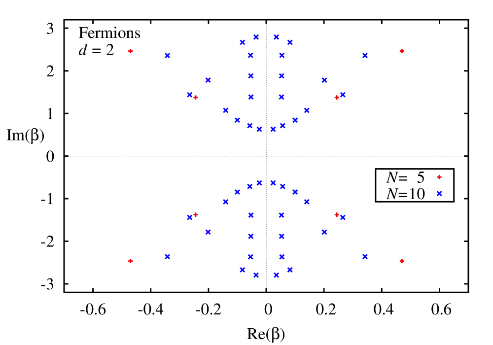
(a)   Zeros of the partition function in two dimensions.

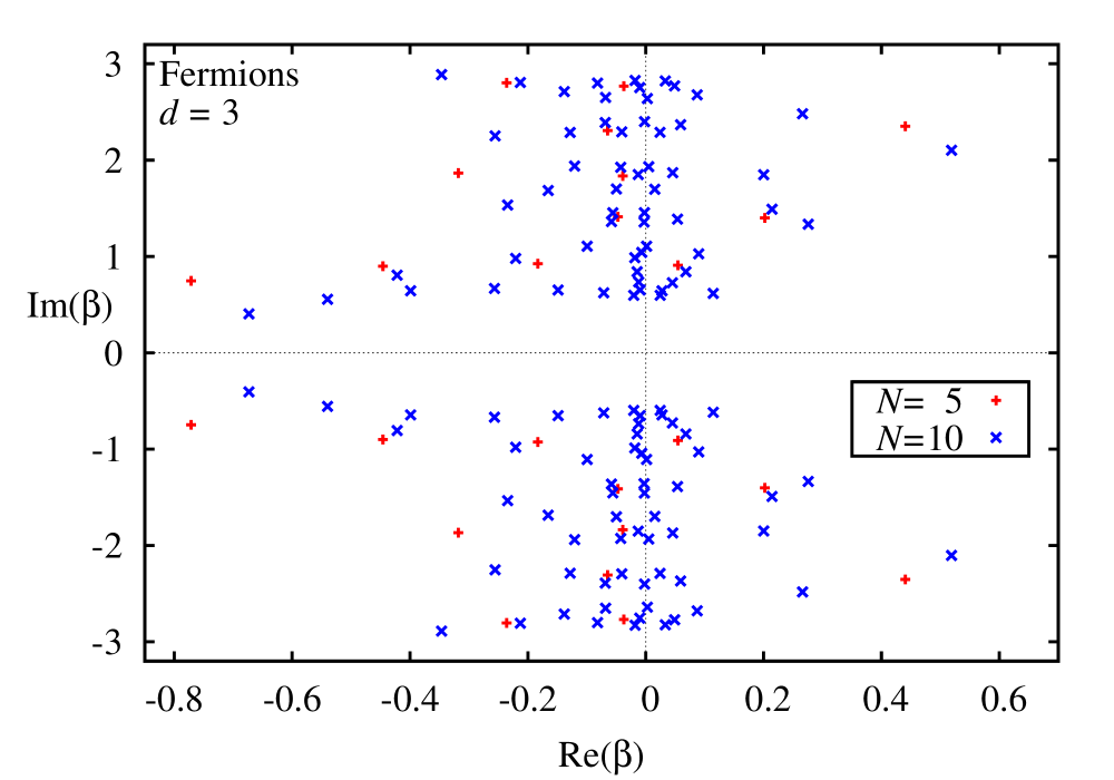
(b)   Zeros of the partition function in three dimensions.

Figure 2: (Color online) The zeros of the exact $Z_{N}(\beta)$, for $N=5$ and $N=10$, obtained from $Z_{1}(\beta)$ of eq. (2) as a function of $\beta=1/kT$ for noninteracting fermions in a harmonic oscillator well: (a) $d=2$ and (b) $d=3$.

In fig. 2, its zeros on the complex plane are displayed for $N=5$ and $N=10$ fermions in two and three spatial dimensions. There are no zeros other than the origin in one dimension. Since $Z_{N}(\beta)$ is known, the thermal properties (for real $\beta$) are easily calculated. These show the expected regular behaviour.

When, however, $Z_{N}(\beta)$ is calculated using $\widetilde{Z}_{1}(\beta)$ given by eq. (5) for the continuous density of states, we get very unexpected results. For even $N$, we find that one zero falls precisely on the positive real $\beta$ axis, even for very small particle number (i.e., $N=2$ ), regardless of the dimension $d$ .

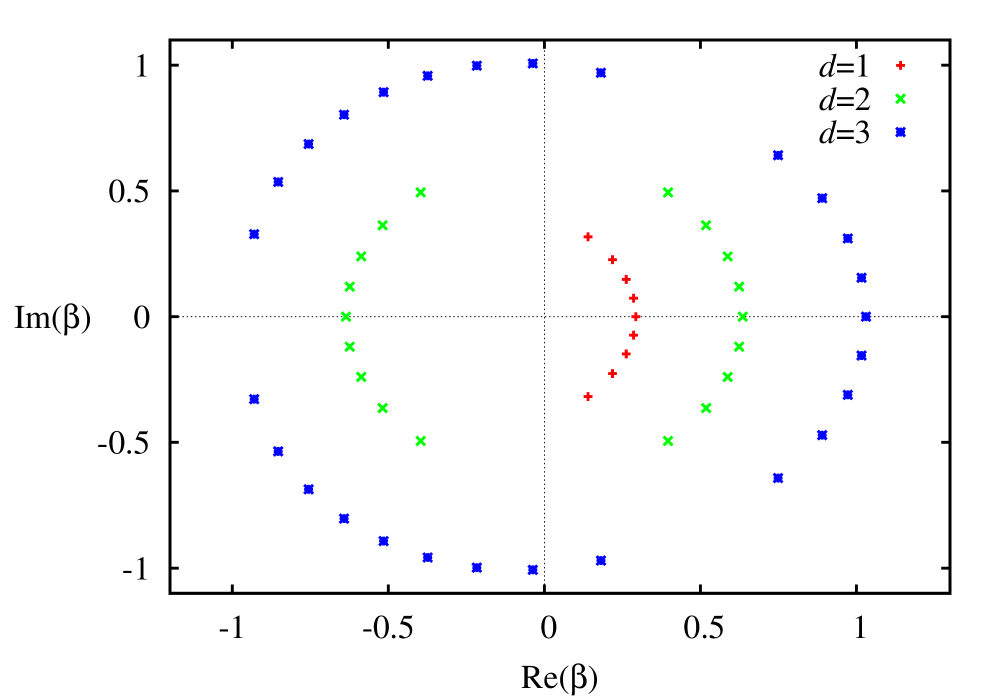
(a)   Zeros of $Z_{N}(\beta)$ for $10$ fermions calculated using $\widetilde{Z}_{1}(\beta)$ given by eq.(5) in three different dimensions.

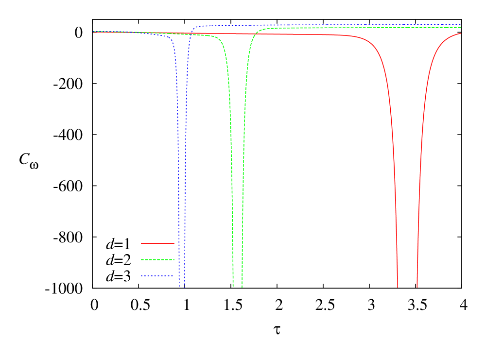
(b)   Heat capacity as a function of temperature for a 10-fermion system, under the same approximation as in (a) above.

Figure 3: (Color online) The zeros of the canonical partition function as a function of $\beta=1/kT$ (a) and the heat capacity as a function of $\tau=1/\beta$ (b) for a system of 10 noninteracting fermions with a continuous density of states, given by eq. (6).

We investigate the thermal properties of such a system when calculated using the canonical formalism. The resulting heat capacity is negative over a range of temperature, indicating instability of the system. This will be discussed shortly. In fig. 3, we display the zeros of $Z_{N}(\beta)$ on the complex $\beta$ plane for $N=10$ in one, two and three spatial dimensions. The associated heat capacities for these cases are also shown. Similar behaviour is also found for very small to very large even $N$. For odd $N$, however, $Z_{N}(\beta)$ from the continuous density of states has no real zero on the positive $\beta$ axis. This could be easily checked analytically, for example, for $N=3$. Nevertheless, the complex zeros of $Z_{N}(\beta)$ get dense near the positive $\beta$ axis and give anomalous thermal properties. This is displayed in fig. 4 for $N=15$. Similar results are obtained for smaller as well as larger odd $N$.

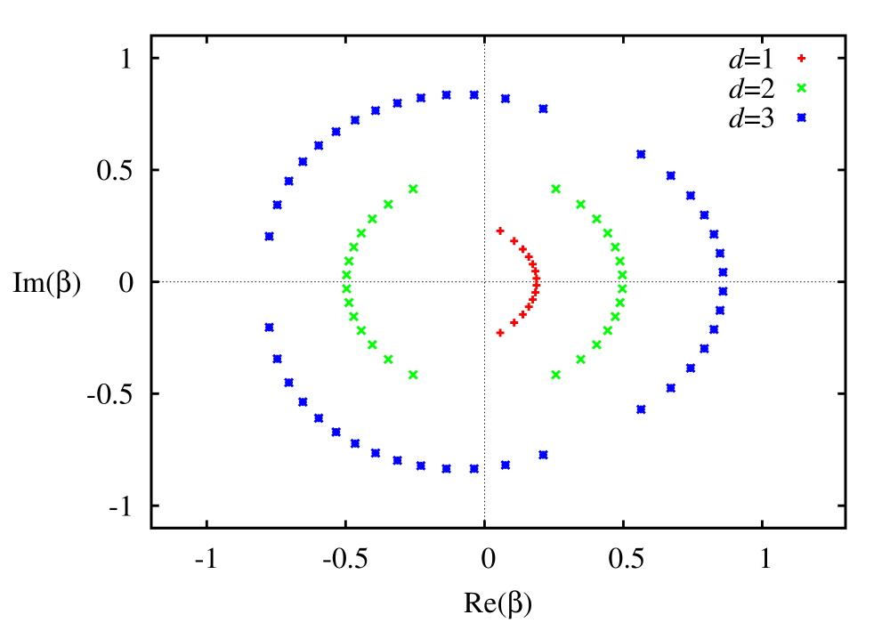
(a)   Zeros of the partition function of 15 fermions for three different dimensions.

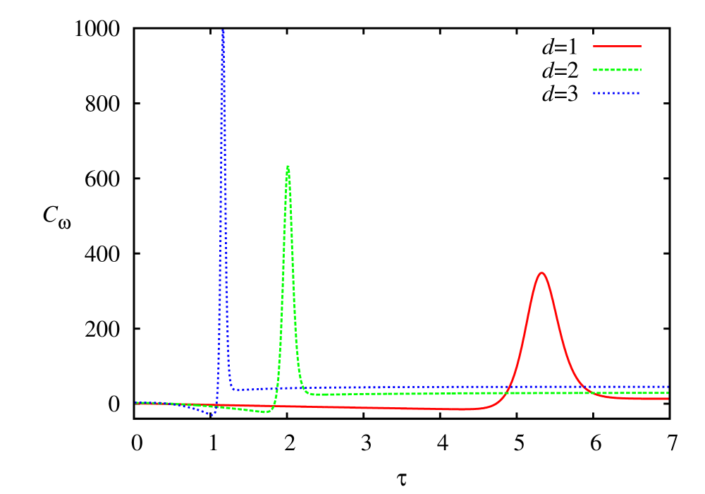
(b)   Heat capacity of a 15-fermion system.

Figure 4: (Color online) The zeros of the canonical partition function as a function of $\beta=1/k_{B}T$ (a) and the heat capacity as a function of $\tau=1/\beta$ (b) for a system of 15 noninteracting fermions with a continuous density of states, given by eq. (6).

The present calculations with the continuous density of states give unphysical results for fermions in a harmonic potential. For example, take the case of $N=2$. From Eq. (1), we get

$$Z_{2}(\beta)=(Z_{1}^{2}(\beta)-Z_{1}(2\beta))/2~{}.$$ (7)

For the continuous density of states, replacing $Z_{1}(\beta)$ by $\widetilde{Z}_{1}(\beta)$, and using Eq. (5) for $d=2$ with $(\hbar\omega=1)$, we obtain

$$\widetilde{Z}_{2}(\beta)=(1/\beta^{4}-1/(4\beta^{2}))/2~{},$$ (8)

which has a real positive root for $\beta=2$. This behaviour for trapped particles is spurious, and can be seen as follows. Consider the single-particle canonical partition function of a one-dimensional system. The $d$-dimensional counterpart may be obtained by taking its $d^{\mathrm{th}}$ power. Writing $Z_{1}(\beta)=\sum_{i}\exp(-\beta\epsilon_{i})$, we find, using Eq.(7)

$$\begin{split}Z_{2}(\beta)&=\frac{1}{2}\left[\sum_{i}\sum_{j}e^{\textstyle-\beta(\epsilon_{i}+\epsilon_{j})}-\sum_{i}e^{\textstyle-2\beta\epsilon_{i}}\right]\\ &=\sum_{i}\sum_{j<i}e^{\textstyle-\beta(\epsilon_{i}+\epsilon_{j})}~{}.\end{split}$$ (9)

The second term on the RHS of Eq. (7) subtracts out the contributions where the two particles occupy the same orbital. The resulting expression for $Z_{2}(\beta)$ in Eq. (9) above is in accordance with the Pauli principle, and cannot be zero for real positive $\beta\neq 0$, if all states have discrete eigenvalues. The roots of $\widetilde{Z}_{2}(\beta)=0$ found from Eq. (8) may not be physically meaningful. This analysis may be extended for larger (finite) $N$. Figure 5 shows the variation of entropy $S$ with temperature for

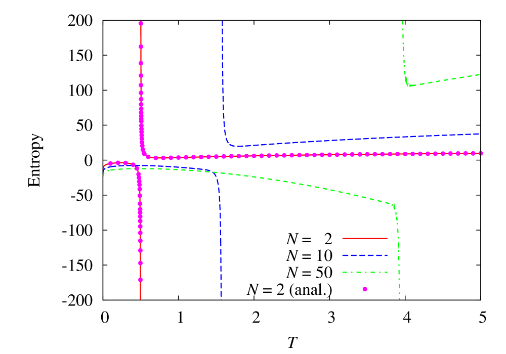
Figure 5: (Color online) Entropy $S$ for 2-dimensional fermion systems with continuous energy-density spectrum. $N=2$ (anal.) refers to entropy obtained from Eq. (8).

$N=2$, $N=10$ and $N=50$ fermions trapped in a $d=2$ harmonic oscillator, using the continuous density of states given by Eq. (6). The behaviour in all three cases is the same, and is dominated by an unphysical pole in $S$ due to the anomalous Fisher zero. Note that the anomalous zero shifts from $T=1/2$ to about $T=4$ as $N$ varies from 2 to 50. For $N=2$, the anomalous zero is at $T=1/2$, and near this $T$, $S\simeq(4T^{2}-1/2)/(T^{2}-1/4)$. This causes $S(T)$ to plunge to large negative values for $T<1/2$, giving rise to a discontinuity at $T=1/2$. This explains why the heat capacity is negative in this range of $T$.

The energy fluctuation in a canonical ensemble is $(\langle E^{2}\rangle-\langle E\rangle^{2})=T^{2}C_{\omega}(T)$, where $\langle\dots\rangle$ denotes an ensemble average. Since the energy fluctuation may also be written as $\langle(E-\langle E\rangle)^{2}\rangle$, we normally expect this to be positive. The change in sign can, however, be explained by examining the inverse Laplace transform of Eq. (8), which gives the two-fermion continuous density of states. This is not positive definite, and ensemble averaging $\langle\dots\rangle$ is no longer guaranteed to yield a positive definite answer. This is easily checked, for example, by calculating, for $E>0$, the ensemble average $\langle E\rangle$ as a function of $T$.

Quite generally, the exact density of states for particles moving in a potential, consists of a smooth continuous part, and a sum of oscillating terms [11]. Equation (3) for the HO is a specially simple example of this. It is the oscillatory contribution that gives rise to the discrete delta-function spikes to the density of states. The oscillatory part has a large effect on the analytical behaviour of $Z_{N}(\beta)$, specially for fermions. The fermionic $Z_{N}(\beta)$ is more sensitive since the recurrence relation given by Eq. (1) has alternating positive and negative terms. This is unlike the situation in the grand canonical partition function, given by

$$\ln Z_{G}(\alpha,\beta)=\int_{0}^{\infty}g(\epsilon)\ln\big{(}1+\exp(\alpha-\beta\epsilon)\big{)}d\epsilon~{},$$ (10)

where $\alpha=\beta\mu$, and $\mu$ the chemical potential. It can be shown that the contribution of the oscillatory terms is exponentially small with a $1/\beta$ dependence in the exponent [15]. The grand canonical formalism generally gives sensible results using the smooth single-particle density of states $\widetilde{g}(\epsilon)$. We show that the same $\widetilde{g}(\epsilon)$, when used recursively to generate the canonical $\widetilde{Z}_{N}(\beta)$, yields anomalous results subject to misinterpretation.

- [1] \NameYang C. N. Lee T. D. \REVIEWPhys. Rev.871952404.
- [2] \NameLee T. D. Yang C. N. \REVIEWPhys. Rev.871952410.
- [3] \NameFisher M. E. in \BookLectures in theoretical physics, edited by \NameBritten W. Vol. 7C (University of Colorado Press, Boulder, Colorado) 1965 pp. 42–45.
- [4] \NameBorrmann P. Franke G. \REVIEWJ. Chem. Phys.9819932484.
- [5] \NameMülken O., Borrmann P., Harting J. Stamerjohanns H. \REVIEWPhys. Rev. A642001013611.
- [6] \NameJanke W. Kenna R. \REVIEWJ. Stat. Phys.10220011211.
- [7] \NameJanke W. Kenna R. \REVIEWNucl. Phys. B (Proc. Suppl.)106-1072002905.
- [8] \NameDas C., Das Gupta S., Lynch W., Mekjian A. Tsang M. \REVIEWPhys. Rep.40620051.
- [9] \NameKenna R., Pinto C. Sexton J. \REVIEWNucl. Phys. B (Proc. Suppl.)832000667.
- [10] \NameBaille C. \REVIEWNucl. Phys. B2831987217.
- [11] \NameBrack M. Bhaduri R. K. \BookSemiclassical physics (Westview Press, Colorado) 2003 p. 122.
- [12] \NamePhillips E. \BookFunctions of a complex variable 8th Edition (Oliver and Boyd, London) 1957.
- [13] \NameAbramowitz M. Stegun I. A. \BookHandbook of mathematical functions (Dover Publications, Inc., New York) 1965 p. 85.
- [14] \NameSchmidt H. J. Schnack J. \REVIEWPhysica A2651999584.
- [15] \NameRichter K., Ullmo D. Jalabert R. A. \REVIEWPhys. Rep.27619961.