The Diagnostics and Possible Evolution in Active Galactic Nuclei Associated With Starburst Galaxies

Abstract

We present a large sample which contains 45 Seyfert 1 galaxies (Sy1s), 46 hidden broad-line region (HBLR) Seyfert 2 galaxies (Sy2s), 57 non-HBLR Sy2s, and 22 starburst galaxies to distinguish their properties and to seek the possible evolution of active galactic nuclei (AGNs) and starburst galaxies. We show that (1) using a plot of [O iii] $\lambda$5007/H$\alpha$ versus [N ii] $\lambda$6584/H$\alpha$ of standard optical spectral diagnostic diagrams, we find that a equation can separate well non-HBLR Sy2s and HBLR Sy2s; (2) the emission-line ratios and both the combination of the ratios and polycyclic aromatic hydrocarbon (PAH) strength are utilized effectively to separate starburst galaxies and Seyfert galaxies; (3) we compare a number of quantities from the data and confirm well the separations with statistics; (4) on the basis of statistics, we suggest that HBLR Sy2s may be the counterparts of Sy1s at edge-on orientation. In addition, we discuss the possibility of starburst galaxies evolving to non-HBLR Sy2s and HBLR Sy2s and then evolving to Sy1s based on the statistical analysis.

1. Introduction

To constrain the galaxy formation and evolution process, it is essential to understand the nuclear activity in nearby galaxies (Constantin et al. 2009). As galaxies evolve, they usually experience the phases of their star formation rates increasing substantially, which is often ascribed to large-scale perturbations in their structure, such as, interactions triggering the formation of bars, resulting in the accumulation of large numbers of gas in their nuclei (Bernard-Salas et al. 2009). For the complexity and importance of the starburst and nuclear activities in the nuclear region, the study of starburst-active galactic nucleus (AGN) connection is a crucial component of modern astrophysics. Based on the results of X-ray imaging and spectroscopic analysis of a Seyfert 2 galaxy (Sy2) sample, starbursts and AGNs are regarded as part of a general evolutionary sequence (Levenson et al. 2001).

Some of the fundamental study for the evolution can date back to the 1980s. Close companions or part of interacting systems were found in the Seyfert galaxies and luminous $Infrared~{}Astronomical~{}Satellite~{}(IRAS)$ galaxies ($L_{\rm FIR}>10^{11}L_{\sun}$; Mirabel $\&$ Wilson 1984; Sanders et al. 1986). In addition, many results indicated that the galaxy interactions play a critical role in boosting not only the far-infrared luminosity but also the $L_{\rm FIR}/M(\rm H_{2})$ ratio (Sanders $\&$ Mirabel 1985; Young et al. 1986), and in the case of strong interactions or mergers, they significantly increase the total supply of molecular gas fueling the starburst. The merger-driven evolutionary sequence initially proposed by Sanders et al. (1988) suggests that the merger of two gas-rich disk galaxies can eventually form an elliptical galaxy.

Based on different methods, some studies seem to conclude that there are indeed some evolutionary processes in some galaxies. Investigating some relations for a sample of 35 Seyfert 2 nuclei, Storchi-Bergmann et al. (2001) found that the star formation activity nearby Seyfert 2 nuclei is linked to interactions and suggested an evolutionary scenario which the starburst dies down with time while the composite Seyfert 2$~{}+~{}$starburst nucleus evolves to a “pure” Seyfert 2 nucleus with an old stellar population. Using the bright infrared galaxies (BIRGs) sample and related studies, Koulouridis et al. (2006) suggested that molecular clouds moving toward the galactic center are drived by close interactions, which can both trigger starburst activity and obscure the nucleus. Under the similar environment found for the BIRGs and Sy2s, Krongold et al. (2002) suggested an evolutionary link between starbursts, Sy2s, and Sy1s and proposed the evolutionary scenrio for AGNs: interaction $\rightarrow$ starburst$\rightarrow$ Seyfert 2 $\leftrightarrow$ Seyfert 1.

Oliva et al. (1999c) found that old and powerful starbursts are absent in Seyfert 1 galaxies while relatively common in obscured (type 2) AGNs. Some studies also show that the majority of type 2 AGNs appear to have experienced significant starbursts (Kauffmann et al. 2003a, b). As suggested in Buchanan et al. (2006) that if star formation is strong in Sy2s, then Seyfert 2 galaxies may evolve to Seyfert 1 galaxies (Tommasin et al. 2010). A similar scenario that Seyfert 2 galaxies are the transitional stages of H ii/starburst galaxies evolving into Seyfert 1 galaxies was proposed: H ii$\rightarrow$ Seyfert 2 $\rightarrow$ Seyfert 1 (Hunt & Malkan 1999; Levenson et al. 2001; Tommasin et al. 2010).

The goal of this study is to explore whether both Seyfert and starburst galaxies can be distinguished by optical and infrared spectral diagnostics; then we investigate and discuss a possibility that whether a evolutionary sequence of starburst galaxies$\rightarrow$ non-hidden broad line region (HBLR) Sy2s $\rightarrow$ HBLR Sy2s $\rightarrow$ Sy1s could be invoked.

This paper is organized as follows. In Section 2, we show the sample of galaxies and their basic properties in detail and provide details of how we selected the data. Section 3 displays the different diagnostics through various quantities. In Section 4, we distinguish between starburst galaxies, non-HBLR Sy2s, HBLR Sy2s, and Sy1s with a number of quantities, namely the optical emission-line ratio, $f_{60}/f_{25}$ ratio, several mid-infrared line ratio diagnostics, and $6.2~{}\mu m~{}$polycyclic aromatic hydrocarbon (PAH) equivalent width (EW) and suggest the possible evolutionary scenario. In Section 5, we discuss the separation among them with the optical and mid-infrared spectral diagnostics, respectively and the possibility of the evolution sequence from starburst galaxies, non-HBLR Sy2s, and HBLR Sy2s to Sy1s. In Section 6, we summarize the results and the conclusions.

Table 1The Sy1 sample

name	$f_{25}$	$f_{60}$	[Ne ii]	[Ne v]	[Ne iii]	[O iv]	[Fe ii]	[S iii]	[Si ii]	$\rm EW$	Reference
			$12.81~{}\mu m$	$14.32~{}\mu m$	$15.56~{}\mu m$	$25.89~{}\mu m$	$25.99~{}\mu m$	$33.48~{}\mu m$	$34.28~{}\mu m$	$6.2~{}\mu m$
(1)	(2)	(3)	(4)	(5)	(6)	(7)	(8)	(9)	(10)	(11)	(12)
ESO 012-G21	0.25	1.45	11.95	3.19	6.42	15.98	…	11.17	26.8	0.278	27,13,13,19
ESO 0141-G55	0.46	0.47	2.24	2.25	5.62	7.26	…	5.45	8.85	…	27,13,13
F03450+0055	0.39	0.87	1.09	$<$1.48	1.82	2.52	…	1.54	$<$4.5	$<$0.103	27,14,14,19
F05563-3820	0.77	0.38	3.89	2.54	4.82	5.31	…	$<$1.84	2.89	….	27,14,14
F13349+2438	0.72	0.85	…	…	…	…	…	…	…	….	27
F15091-2107	0.97	1.60	11.52	8.48	16.29	31.03	…	12.26	12.27	….	27,13,13
IC 4329A	2.26	2.15	27.6	29.3	57.0	117.0	…	16.0	32.5	$<$0.02	27,14,14,19
I ZW 1	1.17	2.24	1.90	5.50	4.50	2.70	$<$1.60	$<$2.00	4.40	0.01	27,15,15,15,18
MCG-2-33-34	0.65	1.23	7.37	6.75	15.93	81.93	…	20.42	29.46	$<$0.304	27,13,13,19
MCG-3-7-11	0.35	1.45	…	…	…	…	…	…	…	…	27
MCG-5-13-17	0.57	1.28	11.0	…	13.0	12.0	…	15.0	…	0.20	27,16,16,19
MCG-6-30-15	0.97	1.39	4.98	5.01	5.88	26.0	…	6.51	9.26	$<$0.063	27,14,14,19
Mrk 6	0.73	1.25	28.0	9.39	49.34	48.24	…	14.09	36.40	$<$0.097	27,13,13,19
Mrk 9	0.44	0.77	3.23	2.21	1.90	5.55	…	3.94	7.32	$<$0.142	1,13,13,19
Mrk 79	0.73	1.55	10.2	6.55	19.6	42.0	…	14.0	30.5	$<$0.039	27,14,14,19
Mrk 205	0.08	0.29	…	…	…	…	…	…	…	…	27
Mrk 231	8.80	35.4	18.50	$<$6.20	$<$5.60	$<$10.00	…	$<$32.50	…	0.011	27,18,18,19
Mrk 279	0.50	1.58	…	3.28	…	10.82	….	…	….	…	27,21
Mrk 335	0.45	0.35	$<$7.0	$<$5.0	$<$8.0	13.0	$<$3.0	$<$1.21	$<$1.45	$<$0.074	27,12,12,14,19
Mrk 509	0.73	1.39	14.0	4.74	14.5	27.5	…	7.41	14.5	0.042	27,14,14,19
Mrk 618	0.85	2.70	16.4	3.89	5.38	10.2	…	6.35	78.0	….	27,14,14
Mrk 704	0.60	0.36	$<$3.30	3.93	5.63	11.8	…	$<$4.30	…	$<$0.071	27,14,14,19
Mrk 817	1.42	2.33	3.83	1.86	4.58	6.53	…	$<$3.21	$<$0.45	$<$0.109	27,13,13,19
Mrk 841	0.47	0.46	3.60	8.0	11.0	24.0	$<$1.0	4.50	5.50	…	1,15,15,15
Mrk 993	$<$0.13	0.30	…	…	…	…	…	…	…	…	1
Mrk 1239	1.21	1.41	9.4	3.4	9.38	15.6	…	9.09	10.5	$<$0.029	27,14,14,19
NGC863	0.22	0.49	…	1.01	…	3.39	…	…	…	….	27,21
NGC931	1.42	2.80	5.47	14.30	15.41	42.60	…	11.97	13.72	$<$0.06	27,13,13,19
NGC1566a	3.07	23.12	21.09	1.19	11.53	7.50	1.56	9.03	18.37	0.223	27,23,23,23,19
NGC3080	$<$0.15	0.35	…	…	…	…	…	…	…	…	27
NGC3227	2.04	9.01	…	23.13	…	65.37	…	19.00	…	0.138	30,21,16,19
NGC3516	0.96	2.09	8.07	7.88	17.72	46.92	…	9.52	22.14	$<$0.061	27,13,13,19
NGC4051	2.28	10.62	21.2	10.7	17.1	94.6	…	38.8	39.6	0.079	27,14,14,19
NGC4151	5.04	5.64	118.0	55.0	207.0	203.0	4.0	81.0	156.0	$<$0.011	27,12,12,12,19
NGC4235	0.28	0.65	…	…	…	…	…	…	…	…	27
NGC4253	1.47	3.89	23.3	21.0	24.1	46.1	…	21.4	15.5	0.036	27,14,14,19
NGC4593	0.96	3.43	7.34	3.09	8.13	33.3	…	19.1	32.2	0.044	27,14,14,19
NGC5548	0.81	1.07	8.47	5.4	7.27	17.5	…	$<$4.14	12.46	0.018	27,14,14,19
NGC5940	0.11	0.74	…	…	…	…	…	…	…	…	27
NGC6104	0.16	0.76	…	…	…	…	…	…	…	…	27
NGC6860	0.31	0.96	5.60	2.85	6.65	12.1	…	7.93	10.4	0.084	27,14,14,19
NGC7213	0.81	2.70	25.7	$<$1.85	12.0	$<$13.5	…	6.97	15.7	0.022	27,14,14,19
NGC7469	6.04	28.57	226.0	$<$15.0	22.0	34.0	6.0	104.0	196.0	0.208	27,12,12,12,18
NGC7603	$<$0.24	0.85	11.0	…	7.0	7.0	…	10.0	…	0.056	1,16,16,19
UGC524	0.17	0.94	…	…	…	…	…	…	…	….	27

Notes: Column 1: Source name. Columns 2 and 3: Infrared flux (in janskys) for 25 and 60 $\mu m$. Columns $4-10$: Flux ($10^{-21}$W $\rm cm^{-2}$) for [Ne ii]  $12.81~{}\mu m$, [Ne v]  $14.32~{}\mu m$, [O iv]  $25.89~{}\mu m$, [Fe ii]  $25.99~{}\mu m$, [S iii]  $33.48~{}\mu m$, and [Si ii] $34.28~{}\mu m$, respectively. Column 11: Equivalent width in $\mu m$. Column 12: References (for columns. 2-3, 4-7, 8, 9-10 and 11, respectively). The fluxes listed of reference 25 between the two high-resolution modules, short-high and long-high, are not to be directly compared because of the different aperture used (Bernard-Salas et al. 2009).

^a Fluxes (except 25 and 60$\mu$m) are listed in units of $\rm 10^{-9}W~{}m^{-2}~{}sr^{-1}$.

This table has the same References as the table 2.

Table 2The HBLR Sy2 sample

name	$\rm\frac{[O~{}III]\lambda 5007}{H\beta}$	$\frac{[\rm N~{}II]\lambda 6584}{H\alpha}$	$f_{25}$	$f_{60}$	[Ne ii]	[Ne v]	[Ne iii]	[O iv]	[Fe ii] a	[S iii]	[Si ii]	$\rm EW$	Reference
					$12.81~{}\mu m$	$14.32~{}\mu m$	$15.56~{}\mu m$	$25.89~{}\mu m$	$25.99~{}\mu m$	$33.48~{}\mu m$	$34.28~{}\mu m$	$6.2~{}\mu m$
(1)	(2)	(3)	(4)	(5)	(6)	(7)	(8)	(9)	(10)	(11)	(12)	(13)	(14)
Circinus	10.25	1.15	68.44	248.7	900.0	317.0	335.0	679.0	59.0	932.0	1510.0	…	20,1,12,12,12
ESO273-IG04	…	…	1.72	4.76	…	…	…	…	…	…	…	…	1
F00521-7054	…	…	0.80	1.02	5.80	5.78	8.13	8.63	…	3.75	…	…	1,13,13
F01475-0740	5.21	0.49	0.84	1.10	13.7	6.38	9.95	6.49	…	3.12	$<$6.13	$<$0.177	4,27,14,14,19
F04385-0828	…	…	1.70	2.91	13.9	2.28	7.06	8.56	…	$<$5.23	$<$5.36	$<$0.058	27,14,14,19
F05189-2524	…	…	3.41	13.27	16.0	19.0	18.0	28.0	3.50	$<$11.0	$<$16.0	0.037	27,15,15,15,19
F11057-1131	…	…	0.32	0.77	…	…	…	…	…	…	…	…	1
F15480-0344	…	…	0.72	1.09	5.57	6.08	9.35	35.0	…	5.20	5.13	$<$0.19	27,14,14,19
F17345+1124	…	…	0.20	0.48	…	…	…	…	…	…	…	…	1
F18325-5926	…	…	1.39	3.23	…	…	…	…	…	…	…	…	1
F20460+1925	…	…	0.53	0.88	…	…	…	…	…	…	…	…	1
F22017+0319	…	…	0.59	1.31	5.95	8.33	14.07	29.04	…	9.33	…	…	27,13,13
F23060+0505	…	…	0.43	1.15	…	…	…	…	…	…	…	…	1
IC 3639	9.55	0.78	2.54	8.90	45.15	11.15	27.00	21.21	…	32.80	44.99	0.185	10,28,13,13,19
IC 5063	8.03	0.60	3.95	5.79	26.7	30.3	66.3	114.0	5.0	31.0	52.7	0.011	6,27,14,12,14,19
MCG-2-8-39	…	…	0.48	0.51	3.86	6.59	9.79	14.4	…	$<$4.31	…	$<$0.128	1,14,14,19
MCG-3-34-64	…	…	2.88	6.22	…	…	…	…	…	…	…	…	27
MCG-3-58-7	…	…	0.98	2.60	8.52	6.63	9.29	8.80	…	$<$2.84	11.7	0.074	27,14,14,19
MCG-5-23-16	0.40	0.78	…	…	…	…	…	…	…	…	…	…	11
Mrk 3	…	…	2.90	3.77	86.0	109.0	207.0	210.0	…	82.0	…	…	1,16,16
Mrk 78	13.09	0.87	0.55	1.11	…	…	…	…	…	…	…	…	7,1
Mrk 348	11.74	0.83	1.02	1.43	16.4	5.82	20.4	17.6	…	12.2	9.81	$<$0.083	20,27,14,14,19
Mrk 463E	…	…	1.49	2.21	11.6	18.3	51.8	72.3	…	13.5	30.3	$<$0.008	27,17,17,19
Mrk 477	…	…	0.51	1.31	…	…	…	…	…	…	…	…	29
Mrk 573	12.3	0.84	0.85	1.24	$<$13.0	18.0	24.0	79.0	…	29.0	…	…	20,24,12,12
Mrk 1210	…	…	2.08	1.89	…	…	…	…	…	…	…	…	1
NGC 424	…	…	1.76	2.00	8.70	16.10	18.45	25.8	$<$3.0	9.82	8.14	$<$0.024	27,13,12,13,19
NGC 513	…	…	0.48	0.41	12.76	1.91	4.43	6.54	1.41	14.50	27.49	0.334	27,13,13,13,19
NGC 591	9.77	1.12	0.45	1.99	…	…	…	…	…	…	…	…	11,1
NGC 788	20.0	0.79	$<$0.51	0.51	…	…	…	…	…	…	…	…	9,1
NGC 1068	13.14	0.82	92.70	198.0	700.0	970.0	1600.0	1900.0	80.0	550.0	910.0	…	20,27,12,12,12
NGC 2110	5.0	1.37	0.84	4.13	…	…	…	…	…	…	…	…	9,1
NGC 2273	5.77	0.86	1.36	6.41	…	16.80	23.8	…	…	…	…	…	8,28,1
NGC 2992	…	…	1.57	7.34	…	…	…	…	…	…	…	0.151	30,19
NGC 3081	…	…	…	…	…	…	…	…	…	…	…	…
NGC 4388	11.15	0.57	3.72	10.46	76.6	46.1	106.0	340.0	…	85.1	135.0	0.128	8,27,14,14,19
NGC 4507	7.14	0.49	1.39	4.31	…	18.40	…	…	…	…	…	…	9,1,1
NGC 5252	5.97	0.88	…	…	…	…	…	…	…	…	…	…	2
NGC 5506	8.91	0.95	4.24	8.44	59.0	26.0	58.0	135.0	6.0	81.0	142.0	0.023	10,27,12,12,12,19
NGC 5995	…	…	1.45	4.09	16.50	6.13	8.47	12.90	…	5.32	25.40	0.066	27,14,14,19
NGC 6552	…	…	1.17	2.57	…	…	…	…	…	…	…	…	27
NGC 7212	12.06	0.69	0.77	2.89	…	…	…	…	…	…	…	…	6,1
NGC 7314	…	…	0.58	3.74	8.08	16.9	23.2	67.0	…	15.0	14.2	0.063	1,14,14,19
NGC 7674	11.75	0.89	1.79	5.64	18.0	31.0	46.0	46.0	…	14.4	29.7	0.132	11,27,16,14,19
NGC 7682	…	…	0.22	0.47	…	…	…	…	…	…	…	…	27
Was 49b	…	…	…	…	…	…	…	…	…	…	…	…

Notes: Column 1: Source name. Columns 2 and 3: Nuclear line ratios. Columns 4 and 5: Infrared flux (in janskys) for 25 and $60~{}\mu m$. Columns $6-11$: Flux ($10^{-21}$W $\rm cm^{-2}$) for [Ne ii]  $12.81~{}\mu m$, [Ne v]  $14.32~{}\mu m$, [O iv]  $25.89~{}\mu m$, [Fe ii]  $25.99~{}\mu m$, [S iii]  $33.48~{}\mu m$, and [Si ii]   $34.28~{}\mu m$, respectively. Column 12: Equivalent width in $\mu m$. Column 13: References (for columns. 2-3, 4-5, 6-9, 10, 11-12 and 13, respectively). The fluxes listed of reference 25 between the two high-resolution modules, short-high and long-high, are not to be directly compared because of the different aperture used (Bernard-Salas et al. 2009).

^a Uncertain detection for NGC 1068 and NGC 5506 (Sturm et al. 2002).

References: (1) NED; (2) MPA-JHU DR7 ; (3) Brandl et al. 2006; (4) Brightman & Nandra 2008; (5) Armus et al. 1989; (6) Bennert et al. 2006; (7) Contini et al, 1998; (8) Ho et al. 1997; (9) Vaceli et al. 1997; (10) Kewley et al. 2000; (11) Veilleux & Osterbrock 1987; (12) Sturm et al. 2002; (13) Tommasin et al. 2008; (14) Tommasin et al. 2010; (15) Veilleux et al, 2009; (16) Deo et al. 2007; (17) Armus et al. 2004; (18) Weedman et al. 2005; (19) Wu et al, 2009; (20) Sosa-Brito et al. 2001; (21) Dasyra et al. 2008; (22) Farrah et al. 2007; (23) Dale et al. 2009; (24) Zhang & Wang 2006; (25) Bernard-Salas et al. 2009; (26) Goulding & Alexander 2009; (27) Tran 2003; (28) Sanders et al. 2003; (29) Imanishi. 2002; (30) Surace et al. 2004;

Table 3The non-HBLR Sy2 sample

name	$\frac{[\rm O~{}III]\lambda 5007}{H\beta}$	$\frac{[\rm N~{}II]\lambda 6584}{H\alpha}$	$f_{25}$	$f_{60}$	[Ne ii]	[Ne v]	[Ne iii]	[O iv]	[Fe ii]	[S iii]	[Si ii]	$\rm EW$	Reference
					$12.81~{}\mu m$	$14.32~{}\mu m$	$15.56~{}\mu m$	$25.89~{}\mu m$	$25.99~{}\mu m$	$33.48~{}\mu m$	$34.28~{}\mu m$	$6.2~{}\mu m$
(1)	(2)	(3)	(4)	(5)	(6)	(7)	(8)	(9)	(10)	(11)	(12)	(13)	(14)
ESO 428-G014	…	…	1.77	4.40	…	82.90	168.01	…	…	…	…	…	24,1
F00198-7926	…	…	1.15	3.10	6.19	12.27	14.03	33.03	…	17.13	…	….	27,13,13
F03362-1642	…	…	0.50	1.06	…	…	…	…	…	…	…	….	24
F04103-2838	…	…	0.54	1.82	11.0	2.50	7.50	4.30	$<$1.00	…	…	….	1,15,15
F04210+0401	…	…	0.25	0.60	…	…	…	…	…	…	…	….	24
F04229-2528	…	…	0.26	0.98	…	…	…	…	…	…	…	….	24
F04259-0440	…	…	1.41	4.13	…	…	…	…	…	…	…	….	1
F08277-0242	…	…	0.43	1.47	…	…	…	…	…	…	…	….	24
F10340+0609	…	…	$<$0.25	0.39	…	…	…	…	…	…	…	….	24
F13452-4155	…	…	0.81	1.84	…	…	…	…	…	…	…	…	24
F19254-7245	…	…	1.35	5.24	31.48	2.77	13.19	6.35	…	9.07	56.80	0.064	27,22,22,19
F20210+1121	…	…	1.40	3.39	…	…	…	…	…	…	…	…	1
F23128-5919	…	…	1.59	10.80	27.29	2.56	20.44	18.16	…	22.47	17.48	….	24,22,22
IC 5298	…	…	1.80	9.76	…	…	…	…	…	…	…	….	24
Mrk 334	…	…	1.05	4.35	30.0	13.0	26.0	15. 0	…	90.0	…	….	1,16,16
Mrk 938	4.0	0.87	2.51	16.84	52.1	$<$2.19	6.37	$<$0.66	…	$<$10.7	40.5	0.44	9,24,14,14,19
Mrk 1066	3.89	0.87	2.26	11.0	…	17.80	52.0	…	…	…	…	…	11,24,1
Mrk 1361	3.41	0.68	0.84	3.28	…	…	…	…	…	…	…	….	2,24
NGC1143	…	…	$<$0.10	$<$1.10	15.0	…	…	…	…	…	…	….	30,1
NGC1144	2.94	0.84	0.62	5.35	17.2	0.92	5.40	5.31	2.51	32.2	67.0	0.343	9,24,14,14,14,19
NGC1241	5.56	0.92	0.60	4.37	13.4	1.61	8.08	5.46	2.41	13.8	19.1	0.461	9,24,14,14,14,19
NGC1320	…	…	1.32	2.21	9.0	8.0	9.0	32. 0	…	12.0	10.4	0.082	24,16,14,19
NGC1358	7.69	1.89	$<$0.12	0.38	…	…	…	…	…	…	…	….	9,24
NGC1386	16.67	1.94	1.46	6.01	17.8	34.5	36.6	106.0	…	31.0	32.8	0.053	9,24,14,14,19
NGC1667	7.58	2.38	0.67	6.29	10.1	1.32	7.23	7.06	…	24.5	54.3	0.391	8,24,14,14,19
NGC1685	…	…	0.22	0.98	…	…	…	…	…	…	…	….	24
NGC3079	…	…	3.65	50.95	98.96	1.31	23.17	8.45	14.57	56.88	173.51	0.458	24,25,25,25,19
NGC3147	6.11	2.71	1.08	8.40	…	…	…	…	…	…	…	…	4,8
NGC3281	10.0	0.98	2.63	6.73	…	…	…	…	…	…	…	…	10,28
NGC3362	8.14	1.74	0.35	2.13	…	…	…	…	…	…	…	….	2,24
NGC3393	10.2	1.2	0.75	2.25	…	42.40	95.0	…	…	…	…	…	20,24,1
NGC3660	2.63	0.82	0.64	2.03	6.51	0.98	1.49	3.61	…	9.52	9.54	$<$0.434	4,27,13,13,19
NGC3982	11.97	0.94	0.97	7.21	11.4	2.89	6.79	5.11	…	15.4	32.8	0.467	2,24,14,14,19
NGC4117	3.98	0.41	…	…	…	…	…	…	…	…	…	….	2
NGC4501	5.25	2.1	3.02	19.93	7.02	$<$1.5	4.72	4.22	2.62	7.9	16.70	$<$0.187	4,27,13,13,13,19
NGC4698	4.29	1.31	$<$0.154	0.26	…	…	…	…	…	…	…	…	8,1
NGC4941	…	…	0.46	1.87	13.50	8.21	24.8	32.8	…	5.79	13.4	$<$0.041	24,14,14,19
NGC5128	…	…	28.2	213.0	221.0	27.0	141.0	98.0	12.0	223.0	545.0	0.014	24,12,12,12,18
NGC5135	3.57	0.85	2.39	16.60	36.7	4.88	16.7	71.3	6.8	38.30	140.0	0.384	9,24,14,14,14,19
NGC5194	8.96	2.90	17.47	108.7	…	…	…	…	…	…	…	0.372	8,8,19
NGC5256	4.47	0.62	1.07	7.25	57.04	7.96	27.95	52.94	4.35	50.93	87.02	0.608	11,28,25,25,25,19
NGC5283	…	…	0.09	0.13	…	…	…	…	…	…	…	…	1
NGC5347	…	…	0.96	1.42	4.17	2.08	4.09	7.64	…	$<$3.38	$<$4.62	$<$0.112	24,14,14,19
NGC5643	11.4	1.04	3.65	19.50	46.41	24.63	56.47	118.28	…	58.0	55.0	…	6,24,26,12
NGC5695	10.47	1.48	0.13	0.57	…	…	…	…	…	…	…	….	11,24
NGC5728	11.8	1.4	0.88	8.16	…	…	…	…	…	…	…	…	20,24
NGC5929	3.42	0.59	1.67	9.52	13.2	1.14	9.83	5.32	…	6.45	21.5	$<$0.48	2,27,14,14,19
NGC6300	9.09	2.23	2.27	14.70	11.52	12.54	15.28	29.45	$<$3.49	$<$7.63	11.31	…	9,24,26,26,26
NGC6890	…	…	0.65	3.85	11.32	5.77	6.57	10.10	…	16.97	26.54	0.237	24,13,13,19
NGC7130	…	…	2.16	16.71	79.3	9.09	29.4	19.7	11.81	48.2	93.9	0.493	28,14,14,14,19
NGC7172	10.0	1.0	0.95	5.74	33.0	10.2	17.1	45.4	…	26.9	59.3	0.045	9,24,14,14,19
NGC7496	0.34	0.46	1.93	10.14	48.08	$<$1.8	6.67	$<$2.4	…	39.47	44.58	0.912	10,28,13,13,19
NGC7582	2.33	0.69	7.48	52.47	148.0	22.0	67.0	116.0	8.0	113.0	218.0	0.274	20,24,12,12,12,19
NGC7590	5.00	1.05	0.89	7.69	7.78	$<$1.5	3.49	5.60	…	15.69	26.50	0.496	9,28,13,13,19
NGC7672	…	…	$<$0.15	0.46	…	…	…	…	…	…	…	….	24
UGC6100	12.63	1.11	0.20	0.57	…	…	…	…	…	…	…	….	2,1

Note: This table has the same Columns and References as the table 2.

Table 4The Starbursts Galaxies sample

name	$\frac{[\rm O~{}III]\lambda 5007}{H\beta}$	$\frac{[\rm N~{}II]\lambda 6584}{H\alpha}$	$f_{25}$	$f_{60}$	[Ne ii]	[Ne v]	[Ne iii]	[O iv]	[Fe ii]	[S iii]	[Si ii]	$\rm EW$	Reference
					$12.81~{}\mu m$	$14.32~{}\mu m$	$15.56~{}\mu m$	$25.89~{}\mu m$	$25.99~{}\mu m$	$33.48~{}\mu m$	$34.28~{}\mu m$	$6.2~{}\mu m$
(1)	(2)	(3)	(4)	(5)	(6)	(7)	(8)	(9)	(10)	(11)	(12)	(13)	(14)
NGC253	0.36	0.72	119.7	784.2	2832.33	$<$20.5	204.64	154.74	250.56	1538.03	2412.03	…	10,1,25,25,25
NGC520	0.74	0.39	3.22	31.52	44.62	$<$0.64	7.53	8.1	7.56	89.44	190.71	0.563	8,3,25,25,25,3
NGC660	2.53	0.85	7.30	65.52	353.01	$<$2.26	36.96	18.8	22.92	246.07	441.96	0.504	8,3,25,25,25,3
NGC1097	5.10	3.0	7.30	53.35	37.24	$<$0.43	6.33	4.41	11.48	100.05	225.19	0.459	20,3,25,25,25,3
NGC1222	2.29	0.21	2.28	13.06	80.57	$<$0.57	89.41	9.92	4.74	132.52	112.05	0.624	10,3,25,25,25,3
NGC1365	3.0	0.55	14.28	94.31	139.50	18.83	59.53	141.57	22.2	246.89	500.3	0.368	20,3,25,25,25,19
IC342	…	…	34.48	180.8	615.46	$<$2.41	37.2	$<$7.7	51.87	672.46	985.73	0.497	3,25,25,25,3
NGC1614	0.81	0.60	7.50	32.12	249.0	$<$0.99	63.32	8.68	12.99	101.06	148.6	0.561	10,3,25,25,25,3
NGC2146	0.48	0.45	18.81	146.69	625.0	$<$2.81	91.16	19.33	52.69	848.02	1209.35	0.545	8,3,25,25,25,3
NGC2623	…	…	1.81	23.74	55.55	2.71	15.08	9.62	2.23	13.78	28.74	0.598	3,25,25,25,3
NGC3256	…	…	15.69	102.63	514.19	$<$2.35	64.42	12.23	33.56	484.64	623.37	0.603	3,25,25,25,3
NGC3310	0.95	0.66	5.32	34.56	27.57	$<$0.25	28.35	4.03	8.78	106.02	143.54	0.789	8,3,25,25,25,3
NGC3556	0.26	0.32	4.19	32.55	21.47	$<$0.37	3.23	$<$1.50	3.14	96.37	96.44	0.502	8,3,25,25,25,3
NGC3628	1.77	0.95	4.85	54.80	125.63	0.9	10.05	$<$2.37	11.96	149.93	277.55	0.50	8,3,25,25,25,3
NGC4088	0.21	0.32	3.45	26.77	37.03	$<$0.39	2.45	0.73	2.15	35.02	63.33	0.496	8,3,25,25,25,3
NGC4194	$\leq$1.35	0.46	4.51	23.20	165.47	2.96	53.99	27.45	8.48	151.01	185.82	0.529	5,3,25,25,25,3
Mrk52	…	…	1.05	4.73	29.38	$<$0.57	3.82	1.31	1.90	60.43	38.02	0.535	3,25,25,25,3
NGC4676	…	…	0.33	2.67	27.78	$<$0.25	4.68	1.37	1.78	23.95	41.27	0.61	3,25,25,25,3
NGC4818	0.15	0.63	4.40	20.12	184.93	$<$1.21	13.73	$<$1.59	10.83	80.54	128.66	0.459	10,3,25,25,25,3
NGC4945	…	…	42.34	625.46	583.84	3.84	68.98	47.85	55.21	338.91	846.23	0.432	3,25,25,25,3
NGC7252	…	…	0.43	3.98	41.68	$<$0.33	3.72	1.33	3.12	24.75	70.53	0.585	3,25,25,25,3
NGC7714	1.35	0.35	2.88	11.16	102.55	$<$1.0	77.42	5.51	5.93	115.9	102.97	0.601	10,3,25,25,25,3

Note: This table has the same Columns and References as the table 2.

2. Sample and Data Reductions

Based on the related analysis between HBLR and non-HBLR Sy2s, Wu et al. (2011) suggested that the former and follower are dominated by AGNs and starburts, respectively. In Section 1, many works showed that Seyfert galaxies could experience some evolution processes. To investigate the evolutionary probability, we define a sample composed of Seyfert and starburst galaxies. However, due to both considering sample completeness and having as large a sample size as possible, this is not an easy job. There are two criteria on sample selection mainly arising from: (1) the spectropolarimetric observations are determinant to distinguish between HBLR and non-HBLR Sy2s; (2) all sources of our multiple subsamples have within $z\sim$0.18. Next we introduce the sample selection of each of our multiple subsamples in detail.

Starburst subsample derives from the study object of Bernard-Salas et al. (2009) which is well known nearby starburst galaxies. Such starburst system often depends on high nuclear star formation rates as the primary energy source. It now seems clear that producing the most luminous infrared galaxies is trigged by strong interactions and mergers of molecular gas-rich spirals and that an important link between starburst galaxies and the AGN phenomena is very likely represented by luminous infrared galaxies (LIRGs; $\geq 10^{11}L_{\sun}$) (Sanders $\&$ Mirabel 1996).

Considering that Mrk 266 and NGC 3079 are suggested by Tran (2003) as non-HBLR Sy2s, so our starburst subsample has 22 objects. Five out of the seven objects with a known AGN component show emission of the high excitation [Ne v] line, meanwhile 15 objects are not signs of AGN activity. In addition, seven of this subsample are LIRGs (Bernard-Salas et al. 2009). In the most luminous of these galaxies, Lagache et al. (2005) suggested that AGN activity is very common, even though their energy output is not dominated by the activity. Based on the above analysis, we have some criteria on sample selection mainly arising from: (1) only those sources have within $z<0.03$; (2) the [Ne v]/[Ne ii]  ratio of $\sim$0.13 is the upper limit.

To avoid the disadvantages of sample misclassification, we try to collect updated and more precise classifications from the literatures. So we mainly employ the combined CfA and 12 $\mu$m sample of Tran (2003) as our Sy1 subsample. Tran (2003) had revised the original Sy1 table of Rush et al. (1993) to include only Sy1 and Sy1.5 galaxies, excluding those classified as Sy1.8 or Sy1.9. In order to avoid biases, he had also removed several highly radio-luminous 3C galaxies from their Sy1 sample, as noted in their table 2. In addition, we exclude NGC 2992 from the Sy1 sample, because the object is classified by NASA/IPAC Extragalactic Database (NED) as a Sy2 galaxy and the spectropolarimetric observation shows that it is an HBLR galaxy (Lumsden et al. 2004).

The Sy1 subsample comprises a subset of the combined 12 $\mu$m and CfA samples of AGNs. To eliminate some forms of selection effects or incompleteness, Rush et al. (1993) followed the approach originated by Spinoglio $\&$ Malkan (1989), a selection based on a flux limit at 12 $\mu$m which minimizes wavelength-dependent selection effects. Using an IRAS detection at 12$\mu$m, $F_{12}(IRAS)>0.22$ Jy, and color selection $F_{60}(IRAS)>0.5F_{12}(IRAS)$ or $F_{100}(IRAS)>F_{12}(IRAS)$ defines the parent sample to remove stars but few galaxies (Rush et al. 1993; Gallimore et al. 2010). The CfA sample had also been defined by Osterbrock $\&$ Martel (1993). So our sample selection mainly meet the following criteria: (1) only those sources have within $z<0.11$; (2) this subsample includes only Sy1 and Sy1.5 galaxies.

Compared to the classical Seyfert 1 galaxies and starburst galaxies, only a small percentage of Sy2s have been observed by spectropolarimetry, and they are not extensively well studied, because this observation is a time-consuming and tedious job (Tran 2001; Wang $\&$ Zhang 2007). Since it is difficult in the spectropolarimetric observations for both HBLR and non-HBLR Sy2s, we have constructed an amalgamated sample by searching all the literatures related to Seyfert galaxy samples.

Some previous samples for studying HBLR and non-HBLR Sy2s are the amalgamation of different observations with diverse quality of spectropolarimetric data (e.g., Gu $\&$ Huang 2002; Zhang $\&$ Wang 2006; Shu et al. 2007), varying from object to object determined by the brightness, observers, integration time, and other factors. For example, although Ruiz et al. (1994) had found that it was no sign for broad H$\alpha$ and H$\beta$ components in the polarized light for Mrk 334, its flux was regarded as polarized broad-line derives from a maximum of $\sim 0.6\%$ of the light in H$\alpha$. For other Sy2s with detected PBLs, the mean percentage of $1\%-5\%$ has been reported. Obviously, it is necessary to evaluate the sensitivities of detecting PBLs in different groups from which our data are taken (Gu $\&$ Huang 2002).

The situation we are faced with has some changes which some groups (e.g., Young et al. 1996; Lumsden et al. 2004; Shi et al. 2010; Tran et al. 2010) have presented detailed information for their polarized broad emission components, so that we can derive their sensitivities — the detected mean polarized broad H$\alpha$ flux is about $2\times 10^{-15}$ergs s^-1 for NGC 3147 and NGC 4698, and their mean percentages of polarized broad H$\alpha$ emission to total H$\alpha$ emission is $0.11\%\pm 0.01\%$ and $0.31\%\pm 0.01\%$, respectively (Tran et al. 2010). However, most sources of our sample have not such comparable sensitivities.

The significant case is the difference in judging either non-HBLR or HBLR Sy2s of two Sy2s (NGC 5347 and NGC 5929). The two sources show faint polarized broad emission lines with high signal-to-noise ratio (S/N) data discovered by Moran et al. (2001), and they were regarded as non-HBLR Sy2s in Tran’s (2001) sample (Gu $\&$ Huang 2002). However, NGC 5929 was also reported as a non-HBLR Sy2 galaxy by Lumsden et al. (2001). Another case is the classification of Mrk 573 which was suggested as a non-HBLR Sy2 galaxy (Tran 2001; 2003), and now it is regarded as an HBLR Sy2 galaxy (Nagao et al. 2004; Ramos Almeida et al. 2008).

Based on the above analysis, the subsamples’ selection of HBLR and non-HBLR Sy2s mainly meet the following criteria: (1) all sources of the two subsamples have within $z\sim$0.18; (2) the percentage of the polarization is $>1\%$ for HBLR Sy2s and $<1\%$ for non-HBLR Sy2s. With regard to their spectropolarimetric observations of HBLR and non-HBLR Sy2s in our sample, Wu et al. (2011) described them (here, Mrk 573 is regarded as an HBLR Sy2 galaxy) in their Table A1 in detail.

Since Seyfert 1 and Seyfert 2 subsamples are included in our sample, we discuss how it would be possible to disentangle evolutionary effects from geometric effects. Baum et al. (2010) found that in Seyfert sample, the opacity of the torus at [Ne v] 14.32 $\mu$m is not large, so we suggest that the [Ne v] 14.32 $\mu$m emission is roughly independent orientation. In addition, [O iv]  25.89 $\mu$m originates purely from the narrow-line region (NLR) in AGNs. In a unified scheme, the NLR line luminosity should be independently orientated (Sturm et al. 2002). Because [Ne v] 14.32 $\mu$m and [O iv]  25.89 $\mu$m are mainly used as the diagnostic of AGNs, we may remove basically their geometric effects in our sample.

To avoid sample bias due to the absence of spectropolarimetric observations, we exclude 18 objects, 4 HBLR Sy2s and 14 non-HBLR Sy2s, from Table 5 in Wang $\&$ Zhang (2007). We construct a sample composed of 170 Seyfert galaxies and starburst galaxies, which contain 45 Sy1s, 46 HBLR Sy2s, 57 non-HBLR Sy2s, and 22 starburst galaxies. The subsample of Sy1s for the combined CfA and 12 $\mu m$ sample is shown in Table 1. The subsamples of HBLR and non-HBLR Sy2s are the amalgamation of different observations with diverse quality of spectropolarimetric data, and they are listed in Tables 2 and 3, respectively. Starburst subsample derives from the study object of Bernard-Salas et al. (2009) and is presented in Table 4.

To improve the accuracy of the measurements of our sample objects, we use the catalog of MPA-JHU emission line measurements for the Sloan Digital Sky Survey (SDSS) Data Release (DR7). The measurements are available for  927552  different spectra. Compared to previous DR4 release, this represents a significant extension in size and a number of improvements in the data. These data are available online at the following address: http://www. mpa-garching. mpg. de/SDSS/DR7/. Each fiber is 3″  in diameter (Bernardi et al. 2003; Adelman-McCarthy et al. 2006). We do cross-correlation with the NED and exclude those objects which are larger than 2″  in RA or DEC errors. According to S/N $>5$ for the H$\beta$ $\lambda$4861, H$\alpha$ $\lambda$6563, [N ii] $\lambda$6584, and [O iii]  $\lambda$5007 lines, meanwhile we exclude the objects with low emission-line signal-to-noise ratio (S/N).

In order to derive reliable statistical results, we have the two highest priorities obtaining a sample which is complete and larger. Since data collected from the literatures or datasets usually involve their different quality, they can also influence the results. In this paper, although they may have some selection effects, we use the line ratios among various fluxes to study Seyfert and starburst galaxies, so the selection effects could little or not influence our results.

3. Derived Quantities

Baldwin, Phillips, & Terlevich (1981) first proposed using optical emission-line ratios to classify the dominant energy source in emission line galaxies. Later, Kewley et al. (2001a) developed the first purely theoretical classification scheme to derive a “starburst line” on the BPT diagrams. However, they had not obtained the accurate line between star forming galaxies and AGNs. To obtain a more stringent sample of star-forming galaxies, Kauffmann et al. (2003b) shifted the Kew01 line to form, Ka03 line, a semi-empirical upper boundary for the star-forming branch observed with the SDSS.

The [O iii] $\lambda$5007/H$\beta$ versus [N ii] $\lambda$6584/H$\alpha$ diagram is most commonly used to separate starburst galaxies from AGN hosts (see e.g., Brinchmann et al. 2004; Lamareille et al. 2004; Mouhcine et al. 2005; Gu et al. 2006). Because dust is often heavily enshrouded nuclei, an important limitation of galaxy optical diagnostic is the effect of extinction. The advent of sensitive infrared line data from the $Infrared~{}Space~{}Observatory~{}(ISO)$ was vital to gazing deeply into buried nuclear sources (Genzel et al. 1998; Laurent et al. 2000a; Sturm et al. 2002; Peeters et al. 2004). Based on the strength of PAH emission features correlating with mid-infrared line ratios, ionization-sensitive indices are first showed by Genzel and collaborators. Spitzer  Space Telescope affords the sensitivity and wide bandpass, so the mid-IR mechanism has a wide prospect (Ho 2008).

The Spitzer  with unprecedented sensitivity and angular resolution can achieve a more detailed view to investigate the nature of galactic nuclei (e.g., Armus et al. 2004; Smith et al. 2004). In Figure 4, we compare the values of [Ne v]  14.32 $\mu m$/[Ne ii]  12.81 $\mu m$ with [O iv]  25.89 $\mu m$/[S iii]  33.48 $\mu m$ measured in our sample of Seyfert galaxies and starburst galaxies. In Figure 5, we investigate the positions of galaxies on the [Fe ii]   25.99 $\mu m$/[O iv]  25.89 $\mu m$ versus [O iv]  25.89 $\mu m$/[S iii]   33.48 $\mu m$ diagnostic diagram. These diagrams separate starburst galaxies from those dominated by AGNs. In Figure 6, since the $f_{60}/f_{25}$ ratio denotes the relative strength of starburst and AGN emissions (Wu et al. 2011), we show the correlation of the $f_{60}/f_{25}$ ratio versus 6.2 $\mu$m EW.

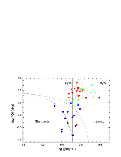
Figure 1.— Traditional diagnostic diagram. Red filled and green open triangles mark HBLR Sy2s and non-HBLR Sy2s; blue filled circles mark starbursts. The dotted curve is the theoretical “maximum starburst line” derived by Kewley et al. (2001a) as an upper limit for star-forming galaxies; the dashed curve on the diagram is the Kauffmann et al.’ (2003a) semi-empirical lower boundary for the star-forming galaxies; the dashed line is Zhang et al. (2008); the red dotted line is described in the text. [See the electronic edition of the Journal for a color version of this figure.]

4. Results

In Section 4.1, we show the separations of starburst galaxies, non-HBLR Sy2s, and HBLR Sy2s with optical diagnostic diagrams. In Section 4.2, their separations are presented by infrared spectral diagnostics and are confirmed by statistics. In Section 4.3, we demonstrate their possible evolution with the change of  [N ii]  flux between starburst galaxies, non-HBLR Sy2s, and HBLR Sy2s/Sy1s.

4.1. Optical Diagnostic Diagrams

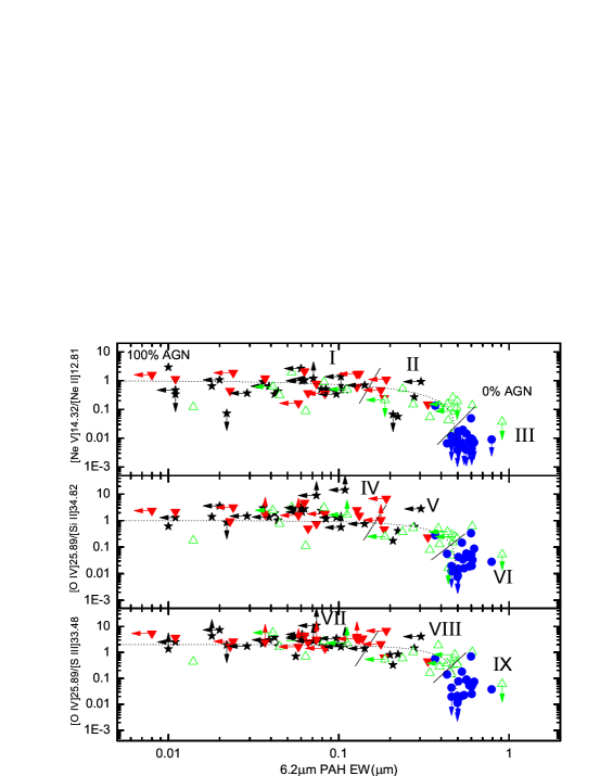
Figure 2.— Ratios of mid-infrared forbidden lines as a function of the $6.2~{}\mu m$ PAH feature equivalent width. Red filled and green open triangles mark HBLR Sy2s and non-HBLR Sy2s, respectively; blue filled circles mark starbursts; black stars mark Sy1s. The dotted lines are linear mixing models of a “pure” AGN and a “pure” star-forming source (see text). The solid lines and Roman numerals delineate regions distinguished by Sy1s, HBLR Sy2s, non-HBLR Sy2s, and starbursts (see table 5). [See the electronic edition of the Journal for a color version of this figure.]

An excellent means of classifying galaxies by easily measured line ratios is provided by the BPT diagnostic diagrams. Here we employ the line ratio of [O iii]   $\lambda$5007/H$\beta$  against the [N ii]  $\lambda$6584/H$\alpha$  ratio. Starburst galaxies fall onto the lower left-hand region of these plots, narrow-line Seyferts are located in the upper right and LINERs are in the lower right-hand zone (Kewley et al. 2001b). We present the diagram for the galaxies of our subsamples in Figure 1 (due to the enough large size of the Sy1s sample of Zhang et al. 2008, we do not put our Sy1s sample into Figure 1). Equations 1 and 2 display the Kewley et al.’s (2001a) theoretical curve (the dotted curve in Figure 1) and Kauffmann et al.’s (2003) semi-empirical curve (the dashed curve), respectively.

$$\rm log(\frac{[OIII]{5007}}{H\beta})=\frac{0.61}{log([NII]/H\alpha)-0.47}+1.19,$$ (1)

$$\rm log(\frac{[OIII]{5007}}{H\beta})=\frac{0.61}{log([NII]/H\alpha)-0.05}+1.3,$$ (2)

$$\rm log(\frac{[OIII]{5007}}{H\beta})=3.53\times log([NII]/H\alpha)+1.65,$$ (3)

Based on the galaxy catalog of SDSS Data Release 4 (DR4) at redshift $z<0.3$, Zhang et al. (2008) found that Seyfert 1 and Seyfert 2 galaxies have different distributions on the [O iii]  $\lambda$5007/H$\beta$  versus [N ii]  $\lambda$6584/H$\alpha$  diagram. Seyfert 2 galaxies display a clear left boundary on the BPT diagram, while Seyfert 1 galaxies do not show such a cutoff. They defined a line (dashed line on this diagram) with the equation 3.

$$\rm log(\frac{[OIII]{5007}}{H\beta})=3.2\times log([NII]/H\alpha)+1.15,$$ (4)

Table 5Classifications by Region in Figure 2

Region	Number of Sources	Sy1s (%)	HBLR Sy2s (%)	non-HBLR Sy2s (%)	Starbursts (%)
(1)	(2)	(3)	(4)	(5)	(6)
I	41	51	32	17	0
II	23	17.5	17.5	61	4
III	23	0	0	9	91
IV	40	50	33	17	0
V	21	19	14	62	5
VI	24	0	0	12	88
VII	43	51	33	16	0
VIII	20	25	20	50	5
IX	26	0	0	19	81

Note: Column 1: the regions in Figure. 2. Column 2: number of Sources. Column 3: the percents in Sy1s. Column 4: the percents in HBLR Sy2s. Column 5: the percents in non-HBLR Sy2s. Column 6: the percents in starburst galaxies.

The non-HBLR Sy2s have weaker optical narrow-line ratios than the HBLR Sy2s on the BPT diagram, so they are closer to the sequence of star-forming galaxies on the BPT diagram (Deo et al. 2009), which appears consistent with that non-HBLR Sy2s are dominated by starbursts (Wu et al. 2011).

In Figure 1, we define the red dotted line with the equation 4 as the separation of HBLR and non-HBLR Sy2s. The line can clearly distinguish between the two types of objects: HBLR Sy2s mainly display a left boundary (12/19) while non HBLR Sy2s mostly display a right boundary (26/30). Compared to non-HBLR Sy2s, HBLR Sy2s are closer to Sy1s in the diagram. Since our sample is not enough completeness, this boundary may not quite accurate and may have no strict physical significance.

4.2. Infrared Spectral Diagnostics of Nuclei and Starburst Regions

4.2.1 Emission-Line Ratios and PAH Strength

Next we use the different emission-line ratios as the mid-infrared diagnostic. The top panel of Figure 2 uses the 6.2 $\mu m$ PAH feature and the emission-line ratio [Ne v] 14.32 $\mu m$/[Ne ii]  12.81 $\mu m$ in a similar mid-infrared diagnostic diagram. Due to the intense star formation in the nuclear region of many active galaxies, some fraction of the measured fluxes of low lying fine structure line (excitation potential $\leq$50 eV) will be produced by photoionization from stars rather than AGNs, while the high excitation lines ([Ne v], [O iv] ) show little or no contamination from possible starburst components (Sturm et al. 2002). Since the ionization potentials needed to product $\rm Ne^{4+}$ and $\rm Ne^{+}$ are 97.1 and 21.6 eV, respectively, the above result can be understood. Starburst galaxies and non-HBLR Sy2s exhibit comparatively large $6.2~{}\mu m$ EWs and relatively low ratios of [Ne v] 14.32 $\mu m$/[Ne ii]  $12.81~{}\mu m$, predicating that the strong contribution comes from [Ne ii]  $12.81~{}\mu m$ and is negligible from AGN emission.

We also use another two diagnostic diagrams in Figure 2. High-ionization lines like [O iv]  25.89 $\mu m$ are somewhat difficult to be detected for its higher ionization potential. Removing an electron from doubly ionized oxygen is required at least $54.9$ eV. Both the middle and bottom panels involve the more easily detectable [Si ii]  34.82 $\mu m$ line which has an ionization potential of 8.15 eV; and another strong mid-infrared lines involved is [S iii]   $33.48~{}\mu m$ with the ionization potentials of 23.3 eV (Dale et al. 2006). In the middle and bottom panels, starburst galaxies and non-HBLR Sy2s exhibit comparatively large $6.2~{}\mu m$ EWs. Starburst galaxies have rough trends in the three panels, which significantly exhibit the comparatively small ratios, so the difference in the ionization potential between various emission lines may be the main factor.

Table 6Classification by Region in Figure 3

Region	Number of Detections	Sy1s (%)	HBLR Sy2s (%)	non-HBLR Sy2s (%)	Starbursts (%)
(1)	(2)	(3)	(4)	(5)	(6)
I	23	61	30	9	0
II	14	36	29	21	14
III	33	18	12	49	21
IV	19	5	5	21	69
I+II	37	51	30	14	5
III+IV	52	14	10	38	38
I+III	56	36	20	32	12
II+IV	33	18	15	21	46

Note: Column 1: parameters. Column 2: number of sources. Column 3: the percents in Sy1s. Column 4: the percents in HBLR Sy2s. Column 5: the percents in non-HBLR Sy2s. Column 6: the percents in starburst galaxies.

Although the starburst galaxies perhaps show a cleaner separation (less mixing), the regions of Figure 2 where Sy1s/HBLR Sy2s/non-HBLR Sy2s mix are slightly significant. According to the unified model of AGNs (Antonucci 1993) and some results (e.g., Tran 2003), it is highly probable that HBLR Sy2s are the counterparts of Sy1s. We can achieve a cleaner separation between Sy1s/HBLR Sy2s and non-HBLR Sy2s. The three regions in the panels of Figure 2 are delineated by the short solid lines roughly perpendicular to the dotted AGN/starburst lines. Using the similar method of Dale et al. (2006), the boundaries are

$\rm log(\frac{[Ne~{}V]14.32~{}\mu m}{[Ne~{}II]12.81~{}\mu m})=10log[EW(6.2~{}\mu m~{}PAH)]+8.0,$

$\rm log(\frac{[Ne~{}V]14.32~{}\mu m}{[Ne~{}II]12.81~{}\mu m})=6.0log[EW(6.2~{}\mu m~{}PAH)]+0.3,$

$\rm log(\frac{[O~{}IV]25.89~{}\mu m}{[Si~{}II]34.82~{}\mu m})=10log[EW(6.2~{}\mu m~{}PAH)]+7.8,$

$\rm log(\frac{[O~{}IV]25.89~{}\mu m}{[Si~{}II]34.82~{}\mu m})=5.0log[EW(6.2~{}\mu m~{}PAH)]+0.8,$

$\rm log(\frac{[O~{}IV]25.89~{}\mu m}{[S~{}III]33.48~{}\mu m})=10log[EW(6.2~{}\mu m~{}PAH)]+8.5,$

$\rm log(\frac{[O~{}IV]25.89~{}\mu m}{[S~{}III]33.48~{}\mu m})=6.0log[EW(6.2~{}\mu m~{}PAH)]+1.5,$

(5)

for regions I-II, II-III, IV-V, V-VI, VII-VIII, and VIII-IX, respectively. The short solid lines separate appropriately Sy1s/HBLR Sy2s, non-HBLR Sy2s, and starburst galaxies. In Table 5, we provide the population statistics for these regions. Regions I+IV+VII and III+VI+IX are representative (at the $>81\%$ level) of Sy1s/HBLR Sy2s and starburst galaxies, respectively, while regions II+V+VIII comprise a some mixture of pure types and are representative (at the $>$50% level ) of non-HBLR Sy2s. Non-HBLR Sy2s exhibit relatively small line ratios and large PAH EWs in Figure 2 (see Table 7), which is consistent with that non-HBLR Sy2s have a quite fraction of starburst components (Wu et al. 2011).

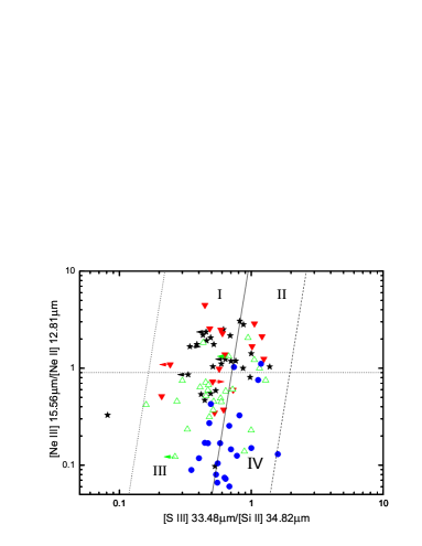
Figure 3.— Neon, Sulfur, and silicon diagnostic diagram involving ratios of lines at different ionizations. The meaning of the symbols is the same as Figure 2. The three lines are defined by the equation 7 and Roman numerals delineate regions distinguished by Sy1s, HBLR Sy2s, non-HBLR Sy2s, and starburst galaxies (see table 6). [See the electronic edition of the Journal for a color version of this figure.]

The dotted lines in Figure 2 display a variational mix both an AGN nucleus and a starburst region. We show the anchors for the mixing model as follow:

$\rm EW(\rm 6.2~{}\mu m~{}PAH)\approx 0.005~{}\mu m$

$\rm(\frac{[Nev]14.32~{}\mu m}{[NeII]12.81~{}\mu m})\approx 1.0(100{\%}~{}AGN)$

$\rm EW(6.2~{}\mu m~{}PAH)\approx 0.5~{}\mu m$

$\rm(\frac{[Nev]14.32~{}\mu m}{[NeII]12.81~{}\mu m})\approx 0.01(0{\%}~{}AGN)$

$\rm EW(\rm 6.2~{}\mu m~{}PAH)\approx 0.005~{}\mu m$

$\rm(\frac{[OIV]25.89~{}\mu m}{[SiII]34.82~{}\mu m})\approx 2.0(100{\%}~{}AGN)$

$\rm EW(6.2~{}\mu m~{}PAH)\approx 0.5~{}\mu m$

$\rm(\frac{[OIV]25.89~{}\mu m}{[SiII]34.82~{}\mu m})\approx 0.02(0{\%}~{}AGN)$

$\rm EW(6.2~{}\mu m~{}PAH)\approx 0.005~{}\mu m$

$\rm(\frac{[OIV]25.89~{}\mu m}{[SIII]33.48~{}\mu m})\approx 2.0(100{\%}~{}AGN)$

$\rm EW(6.2~{}\mu m~{}PAH)\approx 0.5~{}\mu m$

$\rm(\frac{[OIV]25.89~{}\mu m}{[SIII]33.48~{}\mu m})\approx 0.01(0{\%}~{}AGN)$

(6)

These results can be understood. The PAH emission is a tracer of star forming regions in other galaxies (Laurent et al. 2000b; Peeters et al. 2004; Brandl et al. 2006; Dale et al. 2006; Draine et al. 2007; Smith et al. 2007), and its luminosity is in proportion to the star formation rate in star forming galaxies (Roussel et al. 2001; Brandl et al. 2006; Calzetti et al. 2007; Shi et al. 2007; Farrah et al. 2007; Baum et al. 2010). In Figure 2, we know that the 6.2$\mu$m PAH EW is a very useful discriminant between starburst galaxies and Seyfert galaxies.

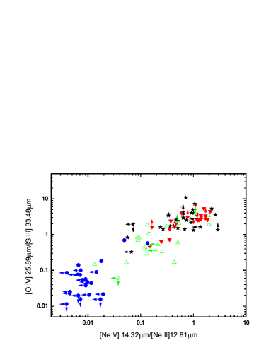
Figure 4.— [Ne v] $14.32~{}\mu m$/[Ne ii] $12.81~{}\mu m$ vs [O iv] $25.89~{}\mu m$/[Ne ii]  $12.81~{}\mu m$ for Seyfert and starburst galaxies in our sample. The meaning of the symbols is the same as Figure 2. A clear positive correlation is observed, representing an excitation sequence anchored with the starburst galaxies, moving up in excitation level to the non-HBLR and HBLR Sy2s, and ending with the Sy1s. [See the electronic edition of the Journal for a color version of this figure.]

4.2.2 A Neon, Sulfur, and Silicon Diagnostic

In Figure 3, we use the similar method of Dale et al. (2006): the neon excitation is regarded as a function of [S iii]  $33.48~{}\mu m$/[Si ii]  $34.82~{}\mu m$, and the separation between the starburst and AGN-powered sources is clear. [Ne iii]  $15.56~{}\mu m$/[Ne ii]  $12.81~{}\mu m$ line ratio is often utilized to interpret the excitation properties of star formation galaxies (Thornley et al. 2000; Verma et al. 2003; Brandl et al. 2006). Since producing $\rm Ne^{+}$ and $\rm Ne^{++}$ needs the ionization potentials of 21.6 and 41.07 eV, respectively, [Ne iii] /[Ne ii]  ratio is sensitive to the most massive stars in a starburst galaxy or to the presence of an AGN (Veilleux et al. 2009). In Figure 3, starburst galaxies and non-HBLR Sy2s exhibit a lower neon excitation while Sy1s and HBLR Sy2s exhibit a higher neon excitation. Table 6 shows the source type fractions within each of the four regions delineated by the lines drawn in Figure 3. The boundaries are defined by lines with the same slope but differing offsets (Dale et al. 2006):

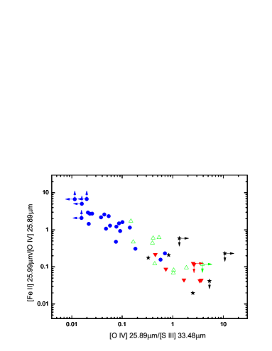
Figure 5.— Mid-infrared diagnostic from Sturm et al. (2006). The meaning of the symbols is the same as Figure 2. [See the electronic edition of the Journal for a color version of this figure.]

$$\rm log(\frac{[NeIII]15.56~{}\mu m}{[NeII]12.81~{}\mu m})=8.4log(\frac{[SIII]33.48~{}\mu m}{[SiII]34.82~{}\mu m})+\gamma,$$ (7)

$\gamma=(+6.5,+1.2,-2.5)$ for the lines demarcating regions (I-II, III-IV).

To estimate the statistical reliability of a classification for a galaxy with the mid-infrared lines, we provide the numbers in Table 6 with the similar means of Dale et al. (2006). In terms of the sample of Dale et al. (2006), this diagram can provide a more significant separation. In Figure 3, Sy1s and HBLR Sy2s mainly appear regions I and II while non-HBLR Sy2s and starburst galaxies mostly reside in regions III and IV. We note, however, that there is scatter in distributions of Sy1s, HBLR Sy2s, and non-HBLR Sy2s.

In Figure 3, Sy1s and HBLR Sy2s will exhibit relatively strong [Si ii]  $34.82~{}\mu m$ emission and somewhat higher [Ne iii]  $15.56~{}\mu m$/[Ne ii]  $12.81~{}\mu m$ ratios. Non-HBLR Sy2s show relatively strong [Si ii]  $34.82~{}\mu m$ emission, while starburst galaxies display strong signatures of [S iii]  $33.48~{}\mu m$ and somewhat lower [Ne iii]   $15.56~{}\mu m$/[Ne ii]  $12.81~{}\mu m$ ratios. In Table 6, it is clear that Region I and IV are representatives (at the $91\%$ and $69\%$ levels, respectively) of Sy1s/HBLR Sy2s and starburst galaxies.

According to the cooling line physics of Dale et al. (2006), these results may be partially understood. The [Si ii]  34.82 $\mu m$ line is a significant coolant of X-ray-irradiated gas (Maloney et al. 1996). AGNs usually have stronger [Si ii]  emission than starburst galaxies, and when [O iv]  is not easily detected, [Si ii]  presents an obvious advantage (Hao et al. 2009). In addition, the [S iii] $33.48~{}\mu m$ line is regarded as a good marker of H ii  regions (Dale et al. 2006). In our subsamples, they are not distinguished with the [S iii] 33.48 $\mu m$/[Si ii]  34.82 $\mu m$. The differences in [S iii] 33.48 $\mu m$/[Si ii]  34.82 $\mu m$ among different subsamples almost are not statistically significant (see Table 7).

In addition, we use the other fine structure line ratios to study the separation of galaxies in our sample. The [O iv]  25.89 $\mu m$/[S iii]  33.48 $\mu m$ and [Ne v]  14.32 $\mu m$/[Ne ii]  12.81 $\mu m$ ratios are considered by us. Since the ionization potentials needed to product $\rm Ne^{4+}$ is 97.1 eV, this [Ne v]  line is detected in 28/44 Sy1s, 25/51 HBLR Sy2s, 32/73 non-HBLR Sy2s, and 5/22 starburst galaxies. [O iv]  25.89 $\mu m$ is also a good indicator of AGN activity ([O iv]   25.89 $\mu m$ is not as good an AGN indicator as the PAH EW, e.g., contaminating [O iv]  emission from WR stars and ionizing shocks, Lutz et al. 1998; Abel & Saryapal 2008; Veilleux et al. 2009). This line is detected in 33/44 Sy1s, 23/51 HBLR Sy2s, 34/73 non-HBLR Sy2s, and 18/22 starburst galaxies (the very low level [O iv]   emission seen in starburst galaxies is not generally attributed to AGN but to either supernova or wind-related ionizing shocks or very hot stars; Lutz et al. 1998; Schaerer & Stasinska 1999). Figure 4 shows a more obvious separation of starburst and AGN-powered sources. The differences in [O iv]  25.89 $\mu m$/[S iii]  33.48 $\mu m$ and [Ne v]  14.32 $\mu m$/[Ne ii]  12.81 $\mu m$ ratios among different subsamples are statistically significant (see Table 7).

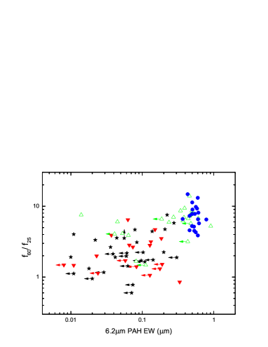
Figure 6.— The $IRAS~{}f_{60}/f_{25}$ flux ratio as a function of the $6.2~{}\mu m$ PAH feature equivalent width. The meaning of the symbols is the same as Figure 2. [See the electronic edition of the Journal for a color version of this figure.]

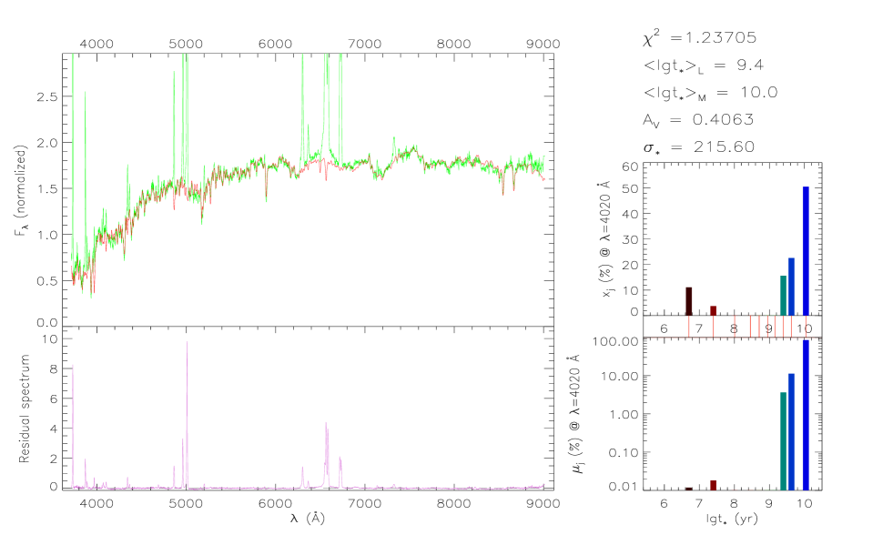
Figure 7.— Spectral synthesis of representative in Sy1 or HBLR Sy2 samples. Left top panel: the observed spectrum $O_{\lambda}$ (green) and the model spectrum $M_{\lambda}$ (red). Left bottom panel: the residual spectrum $E_{\lambda}$ (purple). Right: light (top) and mass (bottom) weighted stellar population fractions $x_{\rm j}$ and $u_{\rm j}$, respectively. The inserted panel on the right marks the ages of the stellar population templates. The flux intensities of the left two panels are normalized at $4020\mathring{\rm A}$.

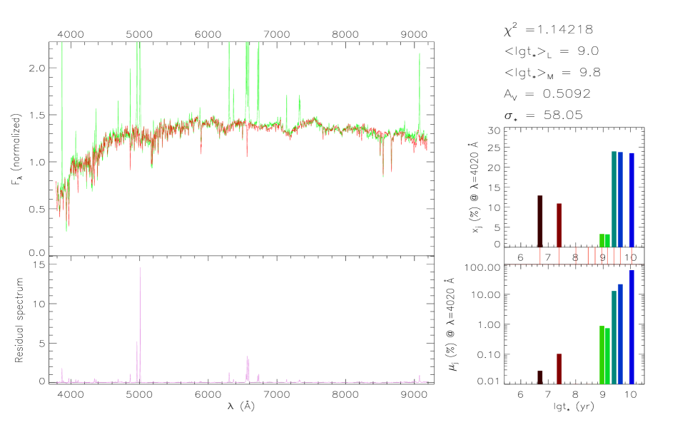
Figure 8.— Spectral synthesis of representative in non-HBLR Sy2 samples. The related description in this Figure is the same as Figure 7.

In Figure 5, we investigate the positions of galaxies on the [Fe ii]   25.99 $\mu m$/[O iv]  25.89 $\mu m$ versus [O iv]  25.89 $\mu m$/[S iii]   33.48 $\mu m$ diagnostic diagram. In the diagram, starburst galaxies are preferentially in upper left corner while HBLR Sy2s/Sy1 have the trend of residing in lower right corner. This diagram can separate well starburst galaxies from those dominated by AGNs. There is scatter in Sy1s distribution, we note, however, the trend may not be change.

These results may be partially understood in the context of [Fe ii]   introduced below. The [Fe ii]  25.99 $\mu m~{}$ and [O iv]  25.89 $\mu m$ lines are observed in starbursts and supernova remnants. In partially ionized zones of shocks, [Fe ii]  is adequately emitted (e.g., Graham et al. 1987; Hollenbach & McKee 1989) and again boosted by shock destruction of grains (e.g., Jones et al. 1996; Oliva et al. 1999a, b) onto which Fe is normally depleted (Lutz et al. 2003). In AGN, compared to the strong [O iv]  emission from the NLR, it is much stronger than the [Fe ii]  emission from shocked or UV/X-ray irradiated partially ionized zones (Lutz et al. 2003).

In Figure 6, we show the $IRAS~{}f_{60}/f_{25}$ flux ratio versus 6.2 $\mu m$ PAH EW. The difference in color between starburt and Seyfert galaxies may be due to the relative strength of the host galaxies and nuclear emissions (Alexander 2001), so Wu et al. (2011) suggested that the $f_{60}/f_{25}$ ratio denotes the relative strength of starbursts and AGN emissions. We find a better correlation of the $IRAS~{}f_{60}/f_{25}$ ratio versus 6.2 $\mu m$ PAH EW with Pearson’s correlation coefficients of 0.59 and a probability of $<$ 0.0001. HBLR Sy2s and Sy1s preferentially appear lower left corner of this diagram while starburst galaxies and non-HBLR Sy2s reside in upper right corner of this diagram. Our results are consistent with those expected for that the $IRAS~{}f_{60}/f_{25}$ flux ratio and EW(6.2 $\mu m$ PAH) are an AGN/SB discriminator.

These ratios can distinguish between starburst galaxies, non-HBLR Sy2s, and HBLR Sy2s/Sy1s. Based on the presentation of Section 2, we can exclude that they could arise from a geometric effects (orientation and solid-angle obscuration). So we suggest that these ratios should show a difference in dominant mechanisms among these galaxies.

4.3. The Probability of Their Evolutionary Sequence

Figure 9.— Spectral synthesis of representative in starburst samples. The related description in this Figure is the same as Figure 7.

4.3.1 Spectral Synthesis

To unveil both the star formation history and the evolution of galaxies, grasping the overall stellar populations of galaxies is vital and essential. Based on the characteristics of circumnuclear stellar populations, Storchi-Bergmann et al. (2001) proposed the evolutionary scenario for Sy2s. To investigate the probability of evolution between starburst and Seyfert galaxies, we utilize their stellar populations to trace their possible evolution.

Since HBLR Sy2s could be the counterparts of Sy1s (Tran 2003), we put HBLR Sy2s into Sy1 subsample. We search all objects of our sample observed by the SDSS and find 6/4, 10, and 3 observed objects which represent Sy1/HBLR Sy2, non-HBLR Sy2, and starburst subsamples, respectively. To derive stellar populations of each of our subsamples, we utilize the spectral synthesis code starlight (Cid Fernandes et al. 2005), which fits the observed spectrum with template spectra of stellar populations and gives the light and mass fractions of each stellar population. starlight also gives the velocity dispersion ($\sigma_{\star}$) of the central region, reddening term $\rm A_{\nu}$, etc. The accuracy and uncertainty of the fitting result had been tested and given by Cid Fernandes et al. (2004, 2005). They combined stellar populations by their ages into “young” ($t_{j}<10^{8}$ yr), “intermediate-age” ($10^{8}\leq t_{j}\leq 10^{9}$ yr) and “old” ($t_{j}>10^{9}$ yr, $t_{j}$ is the age of stellar population) populations, and found that as the signal-to-noise ratio (S/N) increase from 10 to 20, the uncertainty of the young population decreases from 5% to 3%, and the other two populations decrease from 10% to 6%, which suggest that the condensed populations can be well recovered by starlight .

The observed spectra were taken from SDSS Data Release 7. The spectral wavelength coverage is about 3800-8900 Å. All spectra of the subsamples have been corrected for Galactic reddening using dust maps from Schlegel et al. (1998) and also have been corrected for redshift effect. Since the fiber aperture of SDSS spectrographs are 3″, covering the nuclear region, so the fluxes of spectra are mostly come from the bulges of the galaxies.

We adopt simple stellar populations (SSPs) spectra from the Bruzual $\&$ Charlot (2003, hereafter BC03) evolutionary synthesis models as our template spectra and adopt 3 metallicities (Z=0.4, 1, and 2.5$\rm Z_{\sun}$) and 10 ages (0.005, 0.025, 0.1, 0.29, 0.5, 0.9, 1.4, 2.5, 4, and 11 Gyr), which were computed with “Padova 1994” evolutionary tracks (Alongi et al. 1993; Bressan et al. 1993; Fagotto et al. 1994a,b; Girardi et al. 1996) and Chabrier (2003) initial mass function. The metallicities adopted here are representative of neaby galaxies (Gallazzi et al. 2005).

Emission lines [O ii] $\lambda\lambda$3726+3729, [Ne iii] $\lambda$3869, [O iii]  $\lambda\lambda$4959+5007, He i $\lambda$5876, [O i] $\lambda$6300, [N ii] $\lambda\lambda$6548+6583, [S ii] $\lambda\lambda$6716+6731, H$\alpha$, H$\beta$, Na i D5890 galactic interstellar medium absorption line, etc. are all masked and excluded from fitting.

The subsamples selected for stellar population synthesis are those have stellar absorption lines and have S/N $>$ 10. The source numbers of the subsamples (Sy1/HBLR Sy2 subsample, non-HBLR Sy2 subsample, and starburst subsample) are 2/1, 9, and 2, respectively. Figures 7, 8, and 9 present the probable stellar population components of the 3 subsamples given by starlight spectral synthesis result. In each figure, the left-top panel shows the observed SDSS spectrum (green) and the model synthetic spectrum (red); the left-bottom panel gives the residual spectrum (purple); the right-top panel shows the light-weighted fractions $x_{\rm j}$ of the template stellar populations with logarithmic ages $\lg t_{*}$ (yr); the right-bottom panel shows the mass-weighted fractions $\mu_{\rm j}$.

Following Cid Fernandes et al. (2005), we calculate mean ages weighted by the flux and stellar mass as characteristic ages of the nuclear regions:

$\langle\rm lgt_{\star}\rangle_{L}$=$\sum\limits_{j=1}^{N_{\star}}x_{\rm j}\rm lgt_{\rm j}$,

where $x_{j}$ is the light-weighted fraction of each population, and

$\langle\rm lgt_{\star}\rangle_{M}$=$\sum\limits_{j=1}^{N_{\star}}u_{\rm j}\rm lgt_{\rm j}$

where $\mu_{j}$ is the fraction of stellar mass contributed by each SSP. Since the luminosity of a stellar population is very sensitive to young massive stars, so $\langle\lg t_{\star}\rangle_{L}$ can trace recent star formation and evolution history better than $\langle\lg t_{\star}\rangle_{M}$. The statistical mean ages $\overline{\langle\lg t_{\star}\rangle_{L}}$ of the HBLR Sy2s/Sy1s, non-HBLR Sy2s, and starburst galaxies subsamples are $10^{9.3\pm 0.15}$, $10^{8.94\pm 0.18}$, $10^{7.5\pm 0.2}$ yr, respectively. We suggest that, to some extent, these characteristic ages show an evolution sequence of the subsamples.

4.3.2 The Possible Evolution

In Section 4.3.1, we show the age sequence of stellar populations from starburst galaxies to non-HBLR Sy2s and then to HBLR Sy2s/Sy1s. In fact, there are some works to represent indications. Koulouridis et al. (2006) suggested that when the interaction is getting weaker, starburst activity is reduced and an obscured AGN appears simultaneously. Moreover, Wu et al. (2011) found that the non-HBLR Sy2s and HBLR Sy2s are dominated by starbursts and AGNs, respectively, and that there is a list from larger obscuration (non-HBLR Sy2s) to smaller obscuration (HBLR Sy2s). Based on the above analysis, we investigate the probability of evolution sequence from starburst galaxies to non-HBLR Sy2s and then to HBLR Sy2s/Sy1s with another means.

From a purely observational point of view, the BPT diagram is the one of the best distinguishable means for starburst and Seyfert galaxies. We introduce the evolution of galaxies that lie below the dashed Ka03 line. Star-forming galaxies form a tight sequence from low metallicities (low [N ii]/H$\alpha$, high [O iii] /H$\beta$) to high metallicities (high [N ii]/H$\alpha$, low [O iii] /H$\beta$), which were regarded as the “star-forming sequence” (Kewley et al. 2006). The high metallicity end of the star-forming sequence is the beginning of the AGN mixing sequence, and the sequence is extended towards high [O iii] /H$\beta$  and [N ii]/H$\alpha$  values (Kewley et al. 2006; Yuan et al. 2010). This shows that the [N ii]/H$\alpha$  ratio can display well the evolutionary relation in star-forming galaxies, and it may also demonstrate that in some galaxies.

The nitrogen is one of the most abundant elements in the universe, but its nucleosynthesis origin is a long-term puzzle. In term of a primary nucleosynthesis, nitrogen is synthesized by fresh carbon generated by the parent star during hydrogen (H)-burning; in terms of a secondary nucleosynthesis, nitrogen should be synthesized by both carbon and oxygen initially present in the parent star during H-burning, and its abundance is proportional to the initial heavy element abundance (Matteucci 1986). It appears that the abundances of carbon, nitrogen, and oxygen can provide a helpful test for the stellar nucleosynthesis and galactic evolution models.

Based on the chemical evolutionary point of view, the dwarf irregular and blue compact dwarf (BCD) galaxies, the simplest objects assumed commonly, were dealt with in accordance with their chemical evolution in some works (Lequeux et al. 1979; Matteucci & Chiosi 1983; Matteucci & Tosi 1985; Vigroux et al. 1987; Garnett 1990). Although the theory of these galaxies’ chemical evolution is far from being established (Pilyugin 1993), we have achieved some progresses in the related study, and Chiappini et al. (2003) presented the chemical evolution models for dwarf irregulars and spirals, which well reproduce the available constraints for these objects under the supposition that the stellar nucleosynthesis should be the same for all galaxies. Next we demonstrate the possible evolutions in our subsamples.

In Table 7, the mean values of [N ii]/H$\alpha$ ratios increase with the sequence from starburst galaxies to non-HBLR Sy2s and then to HBLR Sy2s. We know that nitrogen is produced during hydrogen burning via the CN or CNO cycles and is known as a primary or secondary element. Primary nitrogen production is largely independent of metallicity and occurs predominantly in intermediate-mass (3-9 $M_{\sun}$) stars (Becker $\&$ Iben 1979, 1980; Renzini $\&$ Voli 1981; Matteucci & Tosi 1985 ; Matteucci 1986); but, some primary nitrogen production derived from massive stars is considered to be dependent on stellar mass and metallicity (Chiappini et al. 2005, 2006; Mallery et al. 2007; Levesque et al. 2010).

Stasi$\rm\acute{n}$ska et al. (2006) suggested that starburst galaxies are dominated by massive stars, and if the stellar populations of circumnuclear in non-HBLR Sy2s are dominated by intermediate-mass stars, then the increase of [N ii]/H$\alpha$  from starburst galaxies to non-HBLR Sy2s can be well understood. Because different mass stars contribute during nitrogen producing the different types of nitrogen (Chiappini et al. 2003), the [N ii]  flux of starburst galaxies is dominated by the secondary nitrogen while that of non-HBLR Sy2s is dominated by the primary nitrogen. With the evolutionary process, the total abundance of nitrogen increases from starbutst galaxies to non-HBLR Sy2s, and the metallicity too. So the [N ii]/H$\alpha$  ratio increases with the list from starburst galaxies to non-HBLR Sy2s.

In addition, we note that the mean values of the ratios decrease with the list from non-HBLR Sy2s to HBLR Sy2s. The reason, we suggest, may be [N ii]  suppressed by a collisional de-excitation process. It is generally accepted that the NLR is stratified that the high-density and high-ionization gas is located close to the nucleus, and low-density and low-ionization gas is in the outer part of the NLR (Tran et al. 2000; Nagao et al. 2003). At the inner NLR, lines with low critical densities, such as [N ii], [S ii], which have the lower ionization potential, are suppressed by a collisional de-excitation process, while lines with high critical densities and recombination lines are unaffected (Zhang et al. 2008). Due to this suppression, it directly causes that the [N ii]/H$\alpha$  ratios decrease with the list from non-HBLR Sy2s to HBLR Sy2s.

At the same time, the [O iii] /H$\beta$  ratio is sensitive to the ionizing radiation field, and the ratio seems to increase with the sequence from starburst galaxies to non-HBLR Sy2s and then to HBLR Sy2s in Table 7. Therefore, the BPT diagram seems to have a hint of the evolutionary sequence from starburst galaxies to non-HBLR Sy2s and then to HBLR Sy2s/Sy1s.

5. Discussions

5.1. Classifications of Nuclei

In this section, we firstly discuss the separation between starburst galaxies, non-HBLR Sy2, and HBLR Sy2 galaxies through the optical diagnostic. Based on the various factors, such as, the metallicity, abundance, the separation can be understood well. Then we discuss the classification between starburst galaxies, non-HBLR Sy2, HBLR Sy2, and Sy1 galaxies through the infrared spectral diagnostic. Table 7 shows the mean values of various quantities and indicates a remarkable separation between Sy1s, HBLR Sy2s, non-HBLR Sy2s, and starburst galaxies utilizing the various methods.

5.1.1 Optical Classification of Nuclei

Table 7Statistical Properties of Starbursts, non-HBLR Sy2s, HBLR Sy2s, and Sy1s

name	parameters	$\rm\frac{[O~{}III]\lambda 5007}{H\beta}$	$\frac{[\rm N~{}II]\lambda 6584}{H\alpha}$	$f_{60}/f_{25}$	[Ne v] /[Ne ii]	[Ne iii] /[Ne ii]	[O iv] /[S iii]	[Fe ii] /[O iv]	[S iii] /[Si ii]	EW
(1)	(2)	(3)	(4)	(5)	(6)	(7)	(8)	(9)	(10)	(11)
S1s(S1)	Mean	…	…	2.83$\pm$0.26	0.76$\pm$0.13	1.35$\pm$0.14	3.27+0.47	0.11$\pm$0.04	0.58$\pm$0.05	0.06$\pm$0.01
	Number	…	…	45	30	32	33	6	27	29
H S2s(S2)	Mean	9.54$\pm$0.94	0.83$\pm$0.05	2.52$\pm$0.19	0.99$\pm$0.12	1.68$\pm$0.22	3.04+0.35	0.09$\pm$0.02	0.67$\pm$0.08	0.08$\pm$0.02
	Number	19	19	42	23	23	23	7	16	18
NH S2s(S3)	Mean	6.93$\pm$0.69	1.27$\pm$0.12	5.20$\pm$0.36	0.38$\pm$0.09	0.75$\pm$0.10	1.41+0.32	0.42$\pm$0.14	0.59$\pm$0.06	0.30$\pm$0.05
	Number	30	30	54	29	29	27	11	25	24
SBs(S4)	Mean	1.37$\pm$0.34	0.70$\pm$0.17	7.52$\pm$0.59	0.013$\pm$0.006	0.27$\pm$0.06	0.11$\pm$0.04	2.34$\pm$0.45	0.70$\pm$0.06	0.54$\pm$0.02
	Number	15	15	22	22	22	22	22	22	21
$p_{\rm null}^{~{}\rm a}(\%)$	S1-S2	…	…	71.20	9.75	27.57	74.56	75.41	32.33	39.81
	S1-S3	…	…	0.00	0.21	0.12	0.01	13.89	77.79	0.01
	S1-S4	…	…	0.00	0.00	0.00	0.00	0.09	14.97	0.00
	S2-S3	4.34	2.14	0.00	0.00	0.03	0.02	5.68	24.06	0.19
	S2-S4	0.00	0.93	0.00	0.00	0.00	0.00	0.01	74.50	0.00
	S3-S4	0.00	0.07	0.11	0.00	0.01	0.00	0.04	11.20	0.00

Notes: Column 1: the types of sources and the probabilities. Column 2: the parameters are Mean, Median, and Number values for the four type objects, perspectively. Columns $3-4$: the flux ratios. Column 5: the $IRAS~{}f_{60}/f_{25}~{}line~{}ratios$. Column $6-10$: the line ratios in [Ne v]  $4.32~{}\mu m$/[Ne ii]  $12.81~{}\mu m$, [Ne iii]  $15.56~{}\mu m$/[Ne ii]  $12.81~{}\mu m$, [O iv]  $25.89~{}\mu m$/[S iii]  $33.48~{}\mu m$, [Fe ii]  $25.99~{}\mu m$/[O iv]  $25.89~{}\mu m$, and [S iii]  $33.48~{}\mu m$/[Si ii]  $34.82~{}\mu m$. Column 11: the $6.2~{}\mu m$ PAH equivalent width (in $\mu m$). S1s, H S2s, NH S2s, SBs denote Sy1s, HBLR Sy2s, non-HBLR Sy2s, and starburst galaxies, respectively.

^a The probability $p_{\rm null}$ (in percent) for the null hypothesis that the two distributions are drawn at random from the same parent population. When there are censored data, we use Peto $\&$ Peto Generalized Wilcoxon Test in ASURV.

In Section 4.1, the [O iii] /H$\beta$  and [N ii]/H$\alpha$  ratios can distinguish between non-HBLR Sy2s, HBLR Sy2s, and starburst galaxies. The distributions of [N ii] $\lambda$6584/H$\alpha$ ratios among them have significant differences. A Kolmogorov-Smirnov (K-S) test shows that all the probabilities for two subsamples of three groups to be extracted from the same parent population are less than $5\%$ (see Table 7). The results can be understood, because the [N ii] $\lambda$6584/H$\alpha$ ratio correlates with both the metallicity and ionization parameter (Veilleux & Osterbrock 1987; Kewley et al. 2001a; Levesque et al. 2010). At lower metallicities, the [N ii] flux is dominated by the abundance of primary nitrogen (Chiappini et al. 2005; Mallery et al. 2007); at higher metallicities, the production of secondary nitrogen becomes prevalent (Alloin et al. 1979; Mallery et al. 2007); carbon and oxygen which originally present in the star synthesize together secondary nitrogen which is thus proportional to abundance (Levesque et al. 2010).

The difference (with a confidence level of $4.34\%$ ) in the [O iii] $\lambda$5007/H$\beta$ ratios between HBLR and non-HBLR Sy2s is presented. We also find the significant differences (with a confidence level of about $10^{\rm-2}$; we adopt the some upper limits as the measured values, since ASURV could not deal with a case that contained both upper and lower limits) in the [O iii] $\lambda$5007/H$\beta$ ratios between starburst galaxies and HBLR or non-HBLR Sy2s. These results can be partial understood, because the [O iii] $\lambda$5007/H$\beta$ ratio is sensitive to the hardness of the ionizing radiation field (Baldwin, Phillips, $\&$ Terlevich 1981) and metallicity (Kewley et al. 2001a).

The basic idea underlying this diagram proposed by Stasi$\rm\acute{n}$ska et al. (2006) is that the emission lines in H ii  regions are powered by massive stars, so the intensities of collisionally excited lines of AGNs are much more than those of starburst galaxies. It indicates that galaxies with AGNs should be prefer in the upper right-hand side of starburst galaxies in the diagram. Obviously, it is consistent with the known results.

5.1.2 Infrared Spectral Diagnostics of Nuclei

Except for the distributions of the [Ne v]/[Ne ii]  and [O iv] /[S iii]   ratios between Sy1s and HBLR Sy2s, Table 7 shows that all the distributions of the two ratios between two subsamples have significant differences. Following Voit (1992) and Spinoglio & Malkan (1992), tracers of the AGN in our sample are the high ionization lines [Ne v]  and [O iv] . With the exception of young Wolf-Rayet stars (Schaerer & Stasi$\rm\acute{n}$ska 1999), the majority of stars do not produce enough energetic photons to excite [Ne v] and [O iv]  (Baum et al. 2010). In addition, the line ratios [Ne v]/[Ne ii]  and [O iv] /[S iii]  have proved empirically to provide a good separation between AGNs and starburst galaxies (Genzel et al. 1998; Sturm et al. 2002; 2006).

The differences in [Ne iii] /[Ne ii]  ratios between two subsamples also are significant, and the K-S test and ASURV tests show that all the probabilities for the two subsamples to be extracted from the same parent population are less than $0.2\%$ with the exception of both Sy1s and HBLR Sy2s (see Table 7). Because of the rather large difference in the ionization potentials of Ne⁺⁺ (41 eV) and Ne⁺ (22 eV), the [Ne iii] /[Ne ii]  ratio is a good tracer of the hardness of the interstellar radiation field (Thornley et al. 2000; Wu et al. 2006). Since the extinction effects on [Ne iii]   $15.56~{}\mu m$ and [Ne ii]  $12.81~{}\mu m$ are similar, the ratio is only weakly affected by extinction (Wu et al. 2006), so the [Ne iii] /[Ne ii]  ratio is a good diagnostic.

Except for the distributions of the [Fe ii] /[O iv]   ratios between Sy1s and HBLR Sy2s, most of the distributions of the ratios between two subsamples are different (the detailed confidence levels for the differences, see Table 7). [Fe ii] $25.99~{}\mu m$ is likely to from fast ionising shocks (Verma et al. 2003), and O’Halloran et al. (2006) suggested that [Fe ii] $25.99~{}\mu m$ emission has been linked primarily to supernova shocks. As mentioned above, the [O iv]  line is correlate with other AGN tracers, so the [Fe ii] /[O iv]  ratio is a distinguishing tool.

There are little differences in the distributions of [S iii] /[Si ii]   ratios between two subsamples. Especially ASURV test shows that a confidence level of $77.79\%$ between non-HBLR Sy2s and Sy1s. Although the exhibition of silicate dust features is speculated generally in the tori, other type 1 AGNs do not show the silicate emission (Sturm et al. 2005). [Si ii]  $34.82~{}\mu m$ line is believed to partly originate in photodissociation regions (PDRs; Sternberg & Dalgarno 1995) and the majority of [Si ii]  emission comes from H ii  regions (Roussei et al. 2007). In addition, many or all of the galaxies have the [S iii]  emission, and it likely originates in star-forming gas (Dudik et al. 2007). In Table 7, the mean values of the [S iii] /[Si ii]  ratios are very close to each other among our subsamples. This indicates that [S iii]  and [Si ii]   emissions may mainly come from H ii  regions of either starburst or Seyfert galaxies.

As a result, our subsamples can be distinguished by the optical and infrared diagnostics. However, the Sy1s and HBLR Sy2s subsamples is an exception. It may indicate that both the Sy1s and HBLR Sy2s come from the same sample, and HBLR Sy2s may be the counterparts of Sy1s at edge-on orientation,

5.2. The Possible Evolution

In this section, we firstly discuss various evolutionary scenarios between Seyfert galaxies and starburst galaxies. Then we discuss that the two models of tidal features and the spectroscopic ages of merger-induced star-forming regions were used as clocks to set the relative ages of the different samples, but they have not been very successful. We also discuss using [N ii]  as the probability of an evolutionary clock.

A supermassive black hole is made through successive mergers among starburst remnants (e.g., Norman & Scoville 1988; Taniguchi et al. 1999; Ebisuzaki et al. 2001; Mouri & Taniguchi 2002b). Galaxy interactions and mergers are fundamental to galaxy formation and evolution. Since galaxy interaction supplies the gas at the high efficiency, although the companion is not recognizable, Seyfert galaxies with circumnuclear starbursts are likely to be interacting (Mouri & Taniguchi 2004). With regard to the merger, the most widely supported merger scenario is based on the Toomre (1977) sequence in which two galaxies lose their mutual orbital energy and angular momentum and then coalesce into a single galaxy. The above-mentioned two actions can supply a high rate of gas required by starbursts and AGNs.

Many works studied and discussed the galaxy evolution, for example, the evolutionary scenario of Heckman et al. (1989) and Osterbrock (1993) can be summarized: starburst galaxies $\rightarrow$ starburst-dominant Seyfert $\rightarrow$ AGN-dominant Seyfert/Sy1s (Mouri & Taniguchi 2002a). Since starbursts in Seyfert galaxies are older than those in classical starburst galaxies, Mouri & Taniguchi (2002a) suggested the evolutionary path of starburst $\rightarrow$ starburst-dominant Seyfert $\rightarrow$ host-dominant Seyfert $\rightarrow$ LINER for a late-type galaxy and another evolutionary path of (starburst$\rightarrow$) AGN-dominant Seyfert $\rightarrow$ host-dominant Seyfert $\rightarrow$ LINER for an early-type galaxy.

Mergers and tidal interactions between galaxies have been studied extensively since the pioneering work of Toomre $\&$ Toomre (1972). Some authors have tried to use tidal features or the spectroscopic ages of merger-induced star-forming regions as clocks to set the relative ages of the different samples. A study of tidal debris associated with 126 nearby red galaxies was presented by van Dokkum (2005) and he concluded that the majority of today’s most luminous field elliptical galaxies were assembled at low redshift through mergers of gas-poor, bulge-dominated systems. These “dry” mergers are consistent with the high central densities of elliptical galaxies, their old stellar populations, and the strong correlations of their properties.

Based on $Spitzer$ MIPS observations, Bai et al. (2010 ) presented the mid-IR study of galaxy groups in the nearby universe and suggested that if galaxy$-$galaxy interactions are responsible, then the extremely low starburst galaxy fraction ($<1\%$) implies a short timescale ($\sim 0.1$ Gyr) for any merger-induced starburst stage. The models of utilizing tidal features and the spectroscopic ages of merger-induced star-forming regions depend strongly on identifying the red tidal features at higher redshift and supposing that the star-forming gas is isothermal, respectively. To date we know that they have not been very successful.

The stellar population in Seyfert 2 is an old stellar content ($>$1Gyr) and has high metallicities (up to three solar; Vaceli et al. 1997), while starburst galaxies have a younger population and show solar metallicities or lower. We analyze the ages of stellar populations in starburst galaxy, non-HBLR Sy2, and HBLR Sy2 subsamples with starlight  respectively, and show them in Figures 7, 8, and 9. Despite the existence of only 14 SDSS-observed objects and poor fittings, we present a probable trend that the ages of stellar population increase with the list from starburst galaxies to non-HBLR Sy2s and then to HBLR Sy2s/Sy1s. Our result is consistent with the known results and we show roughly that HBLR Sy2s have older stellar population than non-HBLR Sy2s. Therefore, our supposition that the stellar populations of circumnuclear in non-HBLR Sy2s are dominated by intermediate-mass stars could be right.

Zhang et al. (2008) presented that Seyfert 1 and Seyfert 2 galaxies have different distributions on the [N ii]/H$\alpha$  versus [O iii] /H$\beta$  diagram and interpreted that it is due to the obscuration of an inner dense NLR by the torus. We argue that this explanation could be unlikely, because it may not account for the difference in [N ii]/H$\alpha$  between HBLR and non-HBLR Sy2s. [N ii] suppressed by a collisional de-excitation process, we suggest, may be the reason of the decrease of the [N ii]/H$\alpha$  ratios. Since non-HBLR Sy2s and HBLR Sy2s are dominated by starbursts and AGNs, respectively (Wu et al. 2011), the [N ii]  flux in non-HBLR Sy2s could be affected less by this collisional de-excitation process or not at all. In addition, our sequence model is agree well with scenarios of Heckman et al. (1989), Osterbrock (1993) and Mouri & Taniguchi (2002a). Certainly, our proposal that uses the metallicity in the form of [N ii]  as a time discriminator should be further verified by other observations.

In Section 5.1, we discuss the classifications between starburst galaxies, non-HBLR Sy2, HBLR Sy2, and Sy1 galaxies through the optical and infrared spectral diagnostic, and we show remarkable separations among them with statistics. In Section 5.2, utilizing the contribution of nitrogen from the different-mass stars and the action of [N ii]  suppressed by a collisional de-excitation process, we may account for the changes of [N ii]  flux in starburst galaxies, non-HBLR S2ys, and HBLR S2ys.

6. Summary

We have carried out the BPT diagram and a detailed study of the mid-infrared emission line properties, which derive from the carefully selected sample of 45 Sy1s, 46 HBLR Sy2s, 57 non-HBLR Sy2s, and 22 starburst galaxies. Using the optical diagnostic, the mid-infrared diagnostic, and PAH EW, we can distinguish among our subsamples. In addition, we also investigate the possible evolution among them. The main results are the followings:

1. We find that the line, $\rm log(\frac{[OIII]{5007}}{H\beta})=3.2\times log([NII]/H\alpha)+1.15$, can well distinguish between non-HBLR Sy2s and HBLR Sy2s on the BPT diagram.

2. The [O iii] /H$\beta$  versus [N ii]/H$\alpha$  diagram can separate Seyfert and starburst galaxies, which is consistent with the known results.

3. In our subsamples, starburst and Seyfert galaxies can be separated by $6.2~{}\mu m$ PAH EW versus the [Ne v] $14.32~{}\mu m$/[Ne ii]  $12.81~{}\mu m$, [O iv]  $25.89~{}\mu m$/[Si ii]  $34.82~{}\mu m$, and [O iv]  $25.89~{}\mu m$/[S iii]  $33.48~{}\mu m$ ratios, respectively.

4. The diagram, [S iii]  $33.48~{}\mu m$/[Si ii]  $34.82~{}\mu m$ against [Ne iii]  $15.56~{}\mu m$/[Ne ii]  $12.81~{}\mu m$, can roughly distinguish among our subsamples.

5. On the basis of statistics, the result that HBLR Sy2s may be the counterparts of Sy1s at edge-on orientation also is consistent with the known results.

6. The [O iii] /H$\beta$  versus [N ii]/H$\alpha$  diagram seems to intimate a evolutionary sequence from starburst galaxies to non-HBLR Sy2s and then to HBLR Sy2s/Sy1s.

From these results we draw the following two main conclusions:

1. The BPT diagram and mid-infrared emission line ratios can distinguish or diagnose well the starburst galaxies, HBLR Sy2s, non-HBLR Sy2s, and Sy1s.

2. A evolutionary sequence of starburst galaxies, non-HBLR Sy2s, HBLR Sy2s, and Sy1s is presented and can be confirmed by using the changes of nitrogen fluxes.

References

- Abel & Saryapal (2008) Abel, N. P., Saryapal, S. 2008, ApJ, 678, 686
- Adelman-McCarthy et al. (2006) Adelman-McCarthy, J. K., et al. 2006, ApJS, 162, 38
- Alexander (2001) Alexander, D. M. 2001, MNRAS, 320, L15
- Alloin, Collin-Souffrin, & Vigroux (1979) Alloin, D., Collin-Souffrin, S., Joly, M., & Vigroux, L. 1979, A&A, 78, 200
- Alongi et al. (1993) Alongi, M., Bertelli, G., Bressan, A., Chiosi, C., Fagotto, F., Greggio, L., & Nasi, E. 1993, A&AS, 97, 851
- Antonucci (1993) Antonucci, R. 1993, ARA&A, 31, 473
- Armus et al. (1989) Armus, L., et al. 1989, ApJ, 347, 727
- Armus et al. (2004) Armus, L., et al. 2004, ApJS, 154, 178
- Bai et al. (2010) Bai, L., et al. 2010, ApJ, 713, 637