THE RELATION BETWEEN DYNAMICS AND
STAR FORMATION IN BARRED GALAXIES

Abstract

We analyze optical and near-infrared data of a sample of 11 barred spiral galaxies, in order to establish a connection between star formation and bar/spiral dynamics. We find that 22 regions located in the bars, and 20 regions in the spiral arms beyond the end of the bar present azimuthal color/age gradients that may be attributed to star formation triggering. Assuming a circular motion dynamic model, we compare the observed age gradient candidates with stellar populations synthesis models. A link can then be established with the disk dynamics that allows us to obtain parameters like the pattern speed of the bar or spiral, as well as the positions of resonance radii. We subsequently compare the derived pattern speeds with those expected from theoretical and observational results in the literature (e.g., bars ending near corotation). We find a tendency to overestimate bar pattern speeds derived from color gradients in the bar at small radii, away from corotation; this trend can be attributed to non-circular motions of the young stars born in the bar region. In spiral regions, we find that $\sim$ 50% of the color gradient candidates are “inverse”, i.e., with the direction of stellar aging contrary to that of rotation. The other half of the gradients found in spiral arms have stellar ages that increase in the same sense as rotation. Of the 9 objects with gradients in both bars and spirals, 6 (67%) appear to have a bar and a spiral with similar $\Omega_{p}$, while 3 (33%) do not.

1 Introduction.

Since the earliest N-body simulations (e.g., Hohl, 1971) established that bars can form in spiral disks, much theoretical work has been undertaken in order to understand their origin and evolution. Theoretical models show that bars can be formed as part of the natural development of the system (Athanassoula, 2009). On the classical view, bars are mainly supported by elongated orbits (called x1 orbits) along the bar major axis (Skokos et al., 2002, and references therein). Chaotic orbits, however, can also support bars in disk galaxies (see, e.g., Voglis et al., 2006a; Harsoula et al., 2011). Given that the stars that make up bars remain most of the time within them, bars, unlike spiral arms, are not density waves (Sparke & Gallagher 2007; see also § 5.3). Bars, however, can also be considered as long-lived waves and “normal” modes in the disk, possibly driving spiral structure (Buta & Combes, 1996).

It has been predicted that single large-scale (“fast”) bars commonly end inside corotation (CR, Contopoulos, 1980; Contopoulos & Papayannopoulos, 1980; Sellwood, 1981), also called Lagrange radius (see, e.g., Sellwood & Wilkinson, 1993). This prediction has also been corroborated by observations (e.g., Merrifield & Kuijken, 1995; Gerssen et al., 1999; Debattista et al., 2002; Aguerri et al., 2003; Fathi et al., 2009; Gabbasov et al., 2009; Corsini, 2010). From these studies, nonetheless, it can also be inferred that the bar’s corotation radius lies between 1 and 1.4 times the bar’s semimajor axis, and not exactly where the bar ends (Aguerri et al., 2003; Buta & Zhang, 2009; Elmegreen, 1996). This may explain why some galaxies (e.g., NGC 1300, NGC 1365, NGC 5236) show dust lanes on the inside of the spiral arms and HII regions on the outside. If bar and arms have the same pattern speed, this makes sense only while spirals lie within corotation (Roberts et al., 1979). A crossing of the dust lanes from the inside to the outside of the arms, marking the corotation position, or an arm bifurcation are also sometimes observed.

Another theory postulates that “slow bars” actually end near the inner Lindblad resonance  (ILR; Pasha & Polyachenko, 1994), and that they are formed by the alignment of elongated and oscillating orbits along the potential (Lynden-Bell, 1979). Combes & Elmegreen (1993) on the other hand, based on the results of numerical models (see also Rautiainen et al., 2005), propose that bars in early Hubble type galaxies (those with high bulge to disk mass ratio) end near CR, whereas those in late type galaxies (with low bulge to disk mass ratio) may end near the ILR, where the spiral arms begin (Elmegreen & Elmegreen, 1989). Nevertheless, “slow” rotating bars are not favored by the comparison of simulations and observations (Schwarz, 1984, 1985; Weiner et al., 2001; Dubinski et al., 2009), probably implying that disks in barred galaxies are maximal (Debattista & Sellwood, 2000). Buta & Zhang (2009) apply the potential-density phase-shift method (Zhang & Buta, 2007) to a near-infrared (NIR) subsample of the Ohio State University Bright Galaxy Survey  (OSUBGS, Eskridge et al., 2002), and also fail to find evidence of the existence of “slow” bars.

Sellwood & Sparke (1988) propose that multiple pattern speeds may be common (see also Sellwood & Wilkinson, 1993; Patsis et al., 2009), such that for some barred galaxies two corotation radii, one belonging to the bar and the other to the spiral arms, may occur simultaneously in the disk. This would imply that spiral arms are connected to bars only transitorily. The possibility also exists that the bar and bulge mask the spiral arms at small radii; the arms would only start to be seen near the bar’s end, creating the impression of a physical connection where there is none. Unsharp masking and/or Fourier-based methods can be used to search for spiral and bar perturbations in the inner parts of galaxies. However, ring-like features at the end of the bar may interfere with the unambiguous identification of a physical connection between bar and arms in some objects.

Rautiainen & Salo (1999) perform simulations that confirm the scenario advanced by Sellwood & Sparke (1988). They also find cases, however, where the bar and spiral rotate with the same pattern speed, as well as other cases where the bar and spiral patterns have different speeds but coupled resonances (Tagger et al., 1987; Masset & Tagger, 1997). In these cases, the bar’s CR may overlap with the spiral 4:1 resonance or ILR, and the bar and spiral arms are indeed connected. Various simultaneous spiral modes are also possible. According to Buta & Zhang (2009), barred galaxies can have “fast” bars (CR at 1 to 1.4 times the bar extent), and spirals rotating at the same or with a different pattern speed. They also consider “super-fast” bars, for which the bar’s CR is well inside the bar’s end and spirals are decoupled, although so far no theoretical models (e.g., n-body or response) have produced a consistent system with CR within the bar.

Observations also indicate that around 20% of early spiral galaxies are double-bar or nested bar systems (Laine et al., 2002; Erwin, 2004, 2009). In these systems, an outer or primary bar harbors an inner or secondary bar in the nucleus. The inner bar rotation is independent from that of the outer bar. There have also been suggestions of triple-bar systems (e.g. NGC 2681, Erwin & Sparke, 1999).

1.1 Star formation

It is commonly observed that giant HII region complexes occur at the end of the bar, where the spiral arms seem to originate (Roberts et al., 1979; Kenney & Lord, 1991). However, not all barred spirals show this feature clearly, and they present $H_{\alpha}$ emission in other regions as well, e.g., along the bar (see García-Barreto et al., 1996). Phillips (1993, 1996) proposes that barred galaxies can be classified according to their star formation properties. Galaxies with Hubble type SBb and “flat” bars have scant star formation in the bar region and a concentration of HII regions in inner rings. Star formation activity can be very high in the circumnuclear region. The second group corresponds to Hubble type SBc and “exponential” bar type. This group has luminous HII regions in the bars, poorly defined rings, and less star formation in the circumnuclear region. In both SBb and SBc galaxies, the star formation rates per unit area seem to be enhanced in the region where the bar joins the spiral arms, more noticeably in the SBb group. Phillips (1996) points out that SBa galaxies tend to show star formation in ring structures, but no star formation activity in the bar and central regions (see also García-Barreto et al., 1996).

According to Athanassoula (1992), gas density enhancements perpendicular and at the end of the bar are often seen in simulations. She also notices that, for bars with “straight” dust lanes, star formation is difficult along the bar because of considerable shear (the situation may be different for curved lanes/shocks). These “straight” dust lanes occur in strongly barred galaxies (Comerón et al., 2009). Regardless of this, Sheth et al. (2000) argue that some stars may be formed between the bar’s end and the circumnuclear region. In their model, stars are born in “dust spurs” on the trailing side of the bar that feed the main dust lanes. Zurita & Pérez (2008), based on $H_{\alpha}$, optical, and NIR observations, find evidence to support this model in the barred spiral NGC 1530. They suggest that stars are formed in the dust spurs and migrate across the bar to its leading side (see also Asif et al., 2005; Elmegreen et al., 2009).

The existence of phase shifts between the $H_{\alpha}$ emission, the old stellar component of the bar, and the CO emission along it has been noticed by Martin & Friedli (1997), Verley et al. (2007), and Sheth et al. (2002). The $H_{\alpha}$ leads both the CO and old stars, although no systematic pattern with galactocentric radius is measured. These observations support the idea that star formation can be triggered in the bar region.

If spiral arms in barred galaxies trigger star formation, then azimuthal color gradients must be observed across them (e.g. Roberts, 1969; González & Graham, 1996; Martínez-García et al., 2009a, b), due to the aging of stars and their velocities relative to the spiral arms. In the cases where spirals corotate with the bar, inverse color gradients (i.e., the direction of stellar aging is contrary to the sense of rotation) are expected.

Age gradients across bars have also been predicted by recent numerical simulations (Dobbs & Pringle, 2010). Moreover, Mazzuca et al. (2008) have detected azimuthal age gradients in $\sim$ half of a sample of 22 nuclear rings, that they speculate may be related to enhanced star formation in the contact points of bar and ring. In the bar region, the mechanisms triggering star formation may be different from the one that sets off star formation in spiral arms, due to the diverse dynamics and shock conditions.

Here, we aim to investigate azimuthal color (age) gradients across bars and spirals in SB (or strong SAB) galaxies, and the connection between these color gradients and bar/spiral dynamics. In figure 1, we show expected sites of color gradients; in this example, the bar ends near corotation (CR) and spiral arms corotate with the bar, which is not necessarily always the case.

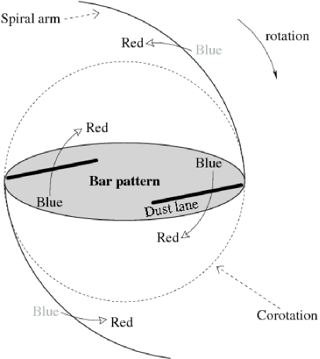
Figure 1: Schematic of stellar age gradients in a barred galaxy. Gradients are shown by arrows that go from blue (young stars) to red (old stars), across a strong bar with straight dust lanes, and through the spiral arms; they are produced by stars born in a shock that then drift away as they age. In this example, the bar ends near CR and the arms corotate with the bar; because the observed arms are completely beyond the CR radius, the spiral pattern overtakes the gas in the disk and the gradients in the arms are “inverse”, that is, the stellar aging vector is opposite to the direction of disk rotation. 

2 Observations

Our sample consists of 11 barred spirals, 9 of them classified as SB, and two as SAB in the Third Reference Catalogue of Bright Galaxies (RC3, de Vaucouleurs et al., 1991). Statistics show that $\sim$30% of spirals are strongly barred in the optical (de Vaucouleurs, 1963; Sellwood & Wilkinson, 1993). In the NIR, Eskridge et al. (2000) find that $\sim$56% are strongly barred (SB) and $\sim$16%, weakly barred (SAB). Their study also shows that late type spirals (Sc-Sm) hold the same fraction of bars as early types (Sa-Sb).

Optical and NIR data were acquired during 1992-1995 with four different telescopes in three observatories: the Cerro Tololo Interamerican Observatory (CTIO) 0.9-m and 1.5-m, the Lick Observatory 1-m, and the Kitt Peak National Observatory (KPNO) 1.3-m telescopes. Deep photometric images were taken in the optical filters $g$, $r$, and $i$, and in the NIR $J$, $K_{s}$ or $K^{\prime}$. Effective wavelengths and widths of all the filters are listed in table 1; the observation log for the 11 galaxies is shown in table 2.

The CTIO 0.9-m optical telescope used a Tek $1024^{2}$ and a Tek $2048^{2}$ CCDs, both with a $0\farcs 4$ pixel^-1 plate scale. The CTIO infrared observations were performed at the 1.5-m telescope, with the Ohio State Infrared Imager/Spectrometer (OSIRIS) in February 1994, and with the CIRIM instrument in September 1994 and September 1995. Both CIRIM and OSIRIS used $256^{2}$ NICMOS3 arrays; the CIRIM focus was adjusted to give a $1\farcs 16$ pixel^-1 plate scale, whereas OSIRIS was used in the $f3$ image mode, that provided a plate scale of $1\farcs 1$ pixel^-1. The CCD at the Lick 1-m telescope was a Ford $2048^{2}$, with a plate scale of $0\farcs 185$ pixel^-1. For the infrared observations at Lick, the same telescope was fitted with the LIRC-2 camera; it had a $256^{2}$ NICMOS II detector, with a $1\farcs 145$ pixel^-1 plate scale. The KPNO infrared observations were made with the IRIM camera, that employed a $256^{2}$ NICMOS3 array, with a $2\arcsec$ pixel^-1 plate scale.

2.1 Data reduction

The data were properly reduced with the image processing package IRAF (Tody, 1986, 1993) and fortran 77 routines. In the optical we applied overscan and trimming corrections. We produced a combined bias frame with the “minmax” rejection algorithm and subtracted it from the data. Dark current frames were inspected, but their counts were found to be negligible. Twilight flats were compared with dome flats, and the former were found to be better. A “master” flat field image was obtained for each filter by scaling flat fields by their median, averaging them with a sigma clipping algorithm, and dividing the result by its mean. Objects were then divided by the appropriate “master” flat. Bad pixels masks were created with the assistance of both dome and twilight flat images. Sky subtraction was achieved by masking bright objects and obtaining the median of the remaining pixels. For some objects the sky emission was not uniform and we fitted a plane, instead of a constant median value. To produce mosaics, individual images were superpixelated by a factor of 2 in each dimension. Each superpixelated frame was inspected for artifacts (e.g., asteroid traces) and the respective pixels were masked. The images were then registered to the nearest pixel (i.e., half an original pixel), and a median mosaic was obtained. Cosmic rays were located and masked by comparing the median mosaic with each individual frame. A final mosaic was then obtained by adding the superpixelated, registered, clean frames.

For the NIR data, we first corrected for the non-linearity of the detector. A polynomial function was adjusted to each pixel of dome flats of increasing exposure times. Source variability and read-out delay time images were used when available, or obtained via iterations. The flat-field correction was done analogously to the optical case. Sky and object frames were taken in an alternating fashion, and with no more than a few minutes difference; sky exposures were centered at different positions with respect to the objects, and separated from them by $\sim$ 10^′, or about twice the linear size of the field-of-view. Bright objects in the sky frames were masked, and the four sky exposures closest in time to each object were median scaled, averaged with a rejection of deviant pixels, scaled to the mean sky value of the object, and subtracted from it; this process also takes care of dark current removal. Flat field corrections were applied with master flats derived from dome flats. Mosaic registering and cosmic ray masking were achieved with the same procedure used for the optical data.

2.2 Calibration

The optical calibration was done in the Thuan-Gunn system (Thuan & Gunn, 1976; Wade et al., 1979). The zero point of this photometric system is chosen such that the standard star BD+17$\arcdeg$4708 has $g=r=i=9.5$. Synthetic magnitudes were obtained for other spectrophotometric standards, using the spectral energy distributions in Oke & Gunn (1983), Stone (1977), Massey et al. (1988), Massey & Gronwall (1990), Hamuy et al. (1992), and Hamuy et al. (1994), and system response curves for each detector/filter/telescope/observatory combination (for details, see Martínez-García et al., 2009a). The best photometric galaxy frame was selected for each object, and the final mosaic was scaled to it. The NIR $J$, $H$ and $K_{s}$ data were calibrated with frames from the Two Micron All Sky Survey (2MASS, Skrutskie et al., 1997, 2006). The $K$ data were calibrated with the Carter & Meadows (1995) photometric standard stars, transformed to the CTIO system (Carter, 1990). For the $K^{\prime}$ data, we adopt $K^{\prime}=K+0.2(H-K)$ (Wainscoat & Cowie, 1992), and use the photometric standard stars of Hawarden et al. (2001). The optical data were degraded to the resolution of the NIR data.

Table 1: Filter characteristics

Filter	$\lambda_{eff}$	FWHM
$g$	5000Å	830Å
$r$	6800Å	1330Å
$i$	7800Å	1420Å
$J$	1.25µm	0.29µm
$H$	1.65µm	0.29µm
$K_{s}$	2.16µm	0.33µm
$K^{\prime}$	2.11µm	0.35µm
$K$	2.2µm	0.41µm

Table 2: Observation Log

Object	Filter	Exposure(s)	Telescope	Date (month/year)	Mean seeing
NGC 718 ……	$g$	8100.	Lick 1 m	10/92, 11/92, 9/93	$2.1\arcsec$
	$r$	7200.	”	10/92, 9/93, 11/93
	$i$	4200.	”	10/92, 9/93
	$J$	672.	Kitt Peak 1.3 m	11/94
	$K_{s}$	336.	”	”
NGC 864 ……	$g$	3865.	Lick 1 m	9/93	$1.7\arcsec$
	$r$	4695.	”	9/93, 11/93
	$i$	3600.	”	11/93
	$J$	1380.	Kitt Peak 1.3 m	9/93, 11/94
	$K_{s}$	360.	”	9/93
NGC 4314 ……	$g$	5400.	Lick 1 m	3/93, 4/93, 4/94	$1.9\arcsec$
	$r$	7599.	”	4/93, 2/94, 4/94
	$i$	2100.	”	2/94, 4/94
	$J$	1252.	Lick 1 m	2/95
	$J$	840.	Kitt Peak 1.3 m	3/94
	$K_{s}$	540.	”	”
NGC 266 ……	$g$	14646.	Lick 1 m	11/92, 9/93, 11/93, 10/94, 11/94	$1.6\arcsec$
	$r$	10165.	”	11/92, 9/93, 10/93, 11/93, 10/94, 11/94
	$i$	6600.	”	11/92, 9/93, 11/93, 10/94, 11/94
	$J$	300.	Kitt Peak 1.3 m	9/93
	$K^{\prime}$	352.	Lick 1 m	12/94
NGC 986 ……	$g$	3600.	CTIO 0.9 m	9/94	$1.5\arcsec$
	$r$	5100.	”	”
	$i$	3900.	”	”
	$J$	810.	CTIO 1.5 m	9/94, 9/95
	$K_{s}$	420.	”	”
NGC 7496 ……	$g$	3600.	CTIO 0.9 m	9/94	$1.6\arcsec$
	$r$	3600.	”	”
	$i$	3600.	”	”
	$J$	300.	CTIO 1.5 m	9/95
	$K_{s}$	330.	”	”
NGC 5383 ……	$g$	2580.	Lick 1 m	4/94, 11/94	$1.4\arcsec$
	$r$	2707.	”	”
	$i$	780.	”	”
	$J$	626.	Lick 1 m	2/95
	$J$	840.	Kitt Peak 1.3 m	3/94
	$K_{s}$	560.	”	”
NGC 4593 ……	$g$	3600.	CTIO 0.9 m	3/94, 3/95	$1.5\arcsec$
	$r$	4500.	”	”
	$i$	4200.	”	”
	$J$	971.	CTIO 1.5 m	2/94
	$K$	868.	”	”
NGC 3059 ……	$g$	4800.	CTIO 0.9 m	3/94, 3/95	$1.6\arcsec$
	$r$	4200.	”	”
	$i$	5400.	”	”
	$J$	313.	CTIO 1.5 m	2/94
	$H$	313.	”	”
NGC 7479 ……	$g$	10620.	Lick 1 m	8/92, 9/93, 10/94	$1.8\arcsec$
	$r$	6960.	”	”
	$i$	8649.	”	”
	$J$	1080.	Kitt Peak 1.3 m	9/93, 11/94
	$K_{s}$	396.	”	”
NGC 3513 ……	$g$	4200.	CTIO 0.9 m	3/94, 3/95	$1.5\arcsec$
	$r$	4500.	”	”
	$i$	4200.	”	”
	$J$	2719.	CTIO 1.5 m	2/94
	$H$	2718.	”	”
	$K$	1042.	”	”

3 Data analysis

The objects were deprojected, by first rotating the frames to align the galaxy’s major axis with the “y” direction, and then stretching the rotated image in the “x” direction by a factor $1/\cos{\alpha}$, where $\alpha$ is the inclination angle. The position and inclination angles were taken from the literature, mostly from Hyperleda (Paturel et al., 2003) and the RC3 (see table 3). The bar and spiral arm perturbations were traced in the NIR bands (mainly $K_{s}$, $K^{\prime}$, and $K$, but other when specified), assuming that young stars do not contribute to the observed radiation (e.g., Rix & Rieke, 1993). However, young stars and clusters may contribute locally up to $20\%-30\%$ to the observed radiation (Rix & Rieke, 1993; González & Graham, 1996; Rhoads, 1998; Patsis et al., 2001; Grosbøl et al., 2006; Grosbøl & Dottori, 2008).

Table 3: Galaxy parameters

Name	Type	PA (deg)	$\alpha$ (deg)	$v_{\mathrm{max}}$ (km s-1)	Radial Velocity (km s-1)	Distance (Mpc)
NGC  718	SAB(s)a	45	$29.4\pm 10.4$	$~{}58.5\pm 14.0$	$1733\pm 10$	$24.3\pm 2.1$
NGC  864	SAB(rs)c	20	$40.7\pm~{}3.1$	$~{}97.9\pm~{}4.1$	$1560\pm~{}4$	$22.0\pm 1.9$
NGC 4314	SB(rs)a	140	$27.0\pm~{}5.3$	$~{}70.6\pm~{}5.0$	$~{}963\pm 26$	$17.7\pm 2.1$
NGC  266	SB(rs)ab	95	$12.2\pm 16.5$	$217.8\pm~{}7.5$	$4661\pm~{}6$	$64.8\pm 5.5$
NGC  986	SB(rs)ab	150	$40.7\pm~{}4.7$	$~{}43.3\pm~{}8.4$	$2005\pm~{}7$	$28.0\pm 2.4$
NGC 7496	SB(s)b	169.7	$24.2\pm~{}9.2$	$~{}65.0\pm~{}6.0$	$1649\pm~{}6$	$23.6\pm 2.0$
NGC 5383	SB(rs)b	85	$31.7\pm~{}6.7$	$142.6\pm 13.1$	$2250\pm~{}4$	$39.2\pm 3.4$
NGC 4593	RSB(rs)b	56	$42.2\pm~{}4.4$	$161.4\pm 10.0$	$2492\pm~{}6$	$38.2\pm 3.3$
NGC 3059	SB(rs)bc	70.9	$27.0\pm~{}8.4$	$~{}55.6\pm~{}5.5$	$1260\pm~{}6$	$15.0\pm 1.3$
NGC 7479	SB(s)c	25	$40.7\pm~{}3.1$	$162.2\pm~{}7.1$	$2378\pm~{}3$	$34.4\pm 2.9$
NGC 3513	SB(rs)c	75	$37.4\pm~{}3.5$	$~{}38.6\pm~{}4.7$	$1194\pm~{}7$	$16.0\pm 1.4$

Note. — Col. (2). Hubble types from RC3. Col. (3). Position angles, mainly from RC3 and Hyperleda (Paturel et al., 2003). Col. (4). Inclination angle, $\alpha=cos^{-1}{(b/a)}$; $a/b$ is the isophotal diameter ratio derived from the $R_{25}$ parameter in RC3. Col. (5). Maximum rotation velocity obtained from the HI data of Paturel et al. (2003), uncorrected for inclination. Col. (6). Heliocentric radial velocity from RC3. Col. (7). Hubble distance obtained from the heliocentric radial velocity and the infall model of Mould et al. (2000), H${}_{0}=71\pm 6$ km s^-1 Mpc^-1.

3.1 Azimuthal color gradient analysis with the GG96 method

The search and analysis of azimuthal color gradients are based on the four band, supergiant sensitive and reddening-free photometric index

$$Q(rJgi)=(r-J)-\frac{E(r-J)}{E(g-i)}(g-i),$$ (1)

where $\frac{E(r-J)}{E(g-i)}$ is the color excess term for a foreground screen. $Q$ is a very good diagnostic of star formation, since its value increases with the presence of blue and red supergiants. Details of the method can be found in González & Graham (1996, GG96 hereafter), and Martínez-García et al. (2009a, b). Briefly, the procedure involves “unwrapping” the spiral arms by plotting them in a $\theta$ vs. ln$R$ map (e.g., Iye et al., 1982; Elmegreen et al., 1992). Under this geometric transformation, logarithmic spirals appear as straight lines with slope = cot(-$i$), where $i$ is the arm pitch angle. The search for color gradient candidates in the bar and arms can be done in the $Q(rJgi)$ “unwrapped” frame, with the aid of a dust lane tracer (e.g., the $g-J$ color). The arms are then “straightened”, by adding a different phase shift at each radius, until the arms appear “horizontal”. In the straightened arms, selected regions can be collapsed in ln $R$ to yield 1-D plots of intensity vs. distance that can be compared with stellar population synthesis (SPS) models.

Stellar models give $Q(rJgi)$ as a function of stellar age ($t_{\rm{age}}$), while observations provide $Q(rJgi)$ as a function of distance. Distance $d=0$ is fixed at the location with the highest extinction (i.e., the highest $g-J$ value) in the dust lane. The pattern speeds of the bar, $\Omega_{p}^{\rm{bar}}$, and of the spiral arms, $\Omega_{p}^{\rm{spiral}}$, are derived from candidates in, respectively, the bar and spiral arm regions, through equation 2, by “stretching” the models to fit the observations (GG96, Martínez-García et al., 2009a):

$$~{}\Omega_{p}\cong\frac{1}{R_{\rm{mean}}}\left(v_{\rm rot}-\frac{d}{t_{\rm age}}-\frac{v_{\rm rad}}{\tan{i}}\right);$$ (2)

$R_{\rm{mean}}$ is the mean radius of the studied region, $v_{\rm{rot}}$ is the galactic rotation velocity from the literature (corrected for inclination; see table 3), $d$ is the azimuthal distance from the shock (i.e., measured from $d=0$), $t_{\rm age}$ is the stellar model age at distance $d$, $v_{\rm rad}$ is the radial velocity, and $i$ is the spiral shock pitch angle, assuming “steady state” (Roberts, 1969). This equation can be easily derived from the one presented in Martínez-García et al. (2009a),

$$\Omega_{p}=\frac{1}{t}\left(\int_{0}^{t}\frac{\vec{v}(t^{\prime})\cdot\hat{\varphi}(t^{\prime})}{R(t^{\prime})}\mathrm{d}t^{\prime}-\left(\theta_{\rm shock}+\Delta\theta\right)\right),$$ (3)

$$\Delta\theta=\cot(i)\ln\left(\frac{R(0)}{R(t)}\right).$$ (4)

Equation 2 assumes nearly circular motion for the involved stellar regions. For the pattern speed determinations we take $v_{\rm rad}\sim 0$, although this term becomes important for tightly wound spirals (see also Grosbøl & Dottori, 2009). Important deviations from circular orbits and velocity gradients are expected in the gas in the azimuthal direction, perpendicular to the bar (Duval & Athanassoula, 1983). Martínez-García et al. (2009b) have shown that, this notwithstanding, azimuthal color gradients across spiral arms can be detected, although assuming a circular motion dynamic model will result in a systematic trend to overestimate spiral pattern speeds at small radii, away from CR, in non-barred or weakly-barred galaxies. Pixel averaging due to image processing compensates in part for this effect (Martínez-García et al., 2009b), such that the measured pattern speed will be correct within the errors, but the systematic trend, whereby the difference between measured and real pattern speeds $\propto R^{-1}$, will still be observed.

3.2 Bar extent

According to Wozniak et al. (1995), the bar end is located after the radius of maximum ellipticity, and is marked by a change in the position angle (PA) of the isophotes. Isophotal PA, on the other hand, must remain roughly constant along the bar region, although spiral structure, rings surrounding the bar, and stellar bar ansae (mainly in early-type galaxies, Martinez-Valpuesta et al., 2007) may disturb the elliptical profiles.

Although the bar extent may be underestimated with the maximum ellipticity criterion (Michel-Dansac & Wozniak, 2006), this method provides a good, homogeneous, standard for our purposes. We determined most bar lengths using the maximum ellipticity criterion (see table 4). To this end, we masked bright stars and nearby objects, and fitted ellipses to the bar’s isophotes (in the NIR, mostly in the 2 $\mu$m, deprojected frames) with the IRAF task ELLIPSE (Jedrzejewski, 1987; Busko, 1996). We then generated plots of isophotal ellipticity and PA versus radius (Wozniak et al., 1995; Mulchaey et al., 1997; Gadotti & de Souza, 2006). The brightest pixel near the nuclear region was given as an initial guess for the isophote center, while re-centering was allowed for outer isophotes. A second “mean isophote center” was computed with these re-centered isophotes; this second center was then used, without allowing for further re-centering. We also performed a visual estimate of the bar’s extension. In figure 2, we compare the results of both measurements.

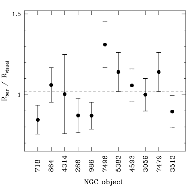
Figure 2: Comparison between the bar extent obtained with the bar’s isophotes ($R_{\rm bar}$, see text), and the estimate by sight ($R_{\rm visual}$). The dashed and dotted lines indicate, respectively, the mean and the error of the ratio of both measurements, 1.02$\pm$0.04. The object numbers in the “New General Catalogue” (NGC, Dreyer, 1888), ordered by Hubble type, are shown in the horizontal axis.

Finally, we compare the bar length with the bar CR radius; the latter is calculated based on the pattern speeds derived from the color gradients in bar regions.

4 Results

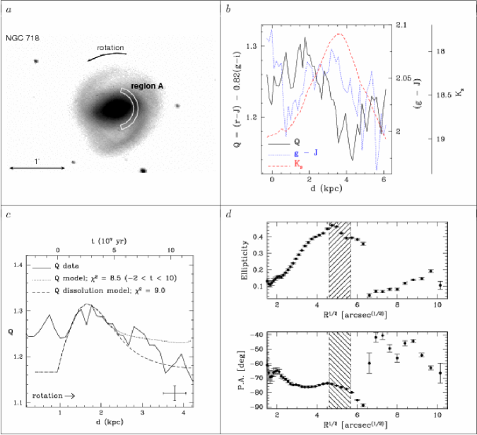
Figure 3: NGC 718, region A. (a.) $g$-band deprojected mosaic of the galaxy, in logarithmic scale. (b.) Solid black line and left y-axis: observed $Q(rJgi)$ profile vs. azimuthal distance, $d$, in kpc; dotted blue line and second-from-right y-axis: observed ($g-J$) color vs. $d$; dashed red line and rightmost y-axis: observed $K_{s}$ surface brightness (mag arcsec^-2) vs. $d$. (c.) Solid line: zoomed-in version of $Q(rJgi)$ vs. $d$ profile. Dotted line: stellar population model, “stretched” in $t_{\rm age}$ to fit the data; IMF $M_{\rm upper}=10M_{\sun}$. Model stellar age, in units of $10^{7}$ yr, is shown in the upper $x$-axis. Dashed line: model including “dissolution of stellar groups”, see §5.1.1. Reduced $\chi^{2}$ values cover the same time interval for both models. (d.) Upper plot: isophote ellipticity vs. $R^{1/2}$; lower plot: isophotal PA vs. $R^{1/2}$. Hatched areas: bar corotation region (see text).

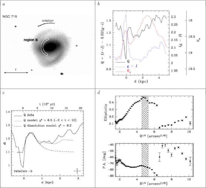
Figure 4: NGC 718, region B. (c.) Dotted and dashed lines: stellar population models, IMF $M_{\rm upper}=10M_{\sun}$.

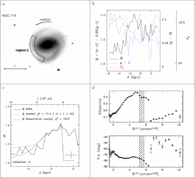
Figure 5: NGC 718, region C. (c.) Dotted and dashed lines: stellar population models, IMF $M_{\rm upper}=100M_{\sun}$.

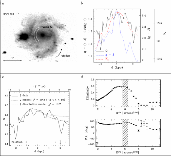
Figure 6: NGC 864, region A. (c.) Dotted and dashed lines: stellar population models, IMF $M_{\rm upper}=10M_{\sun}$.

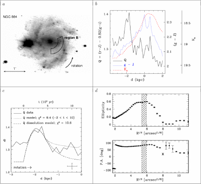
Figure 7: NGC 864, region B. (c.) Dotted and dashed lines: stellar population models, IMF $M_{\rm upper}=10M_{\sun}$.

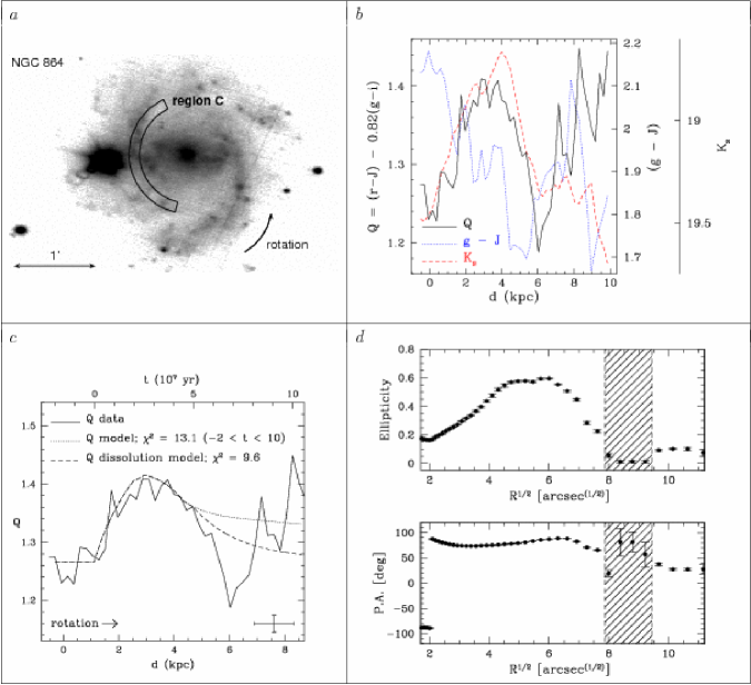
Figure 8: NGC 864, region C. (c.) Dotted and dashed lines: stellar population models, IMF $M_{\rm upper}=10M_{\sun}$.

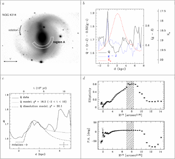
Figure 10: NGC 4314, region A. (a): optical $r$ mosaic. (c.) Dotted and dashed lines: stellar population models, IMF $M_{\rm upper}=10M_{\sun}$.

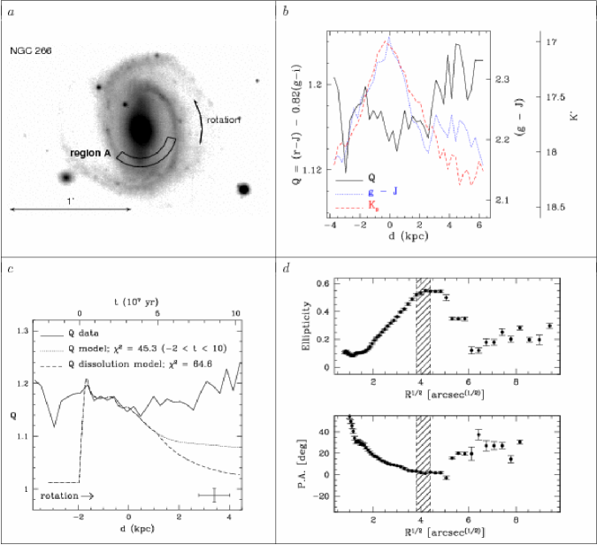
Figure 12: NGC 266, region A. (c.) Dotted and dashed lines: stellar population models, IMF $M_{\rm upper}=100M_{\sun}$.

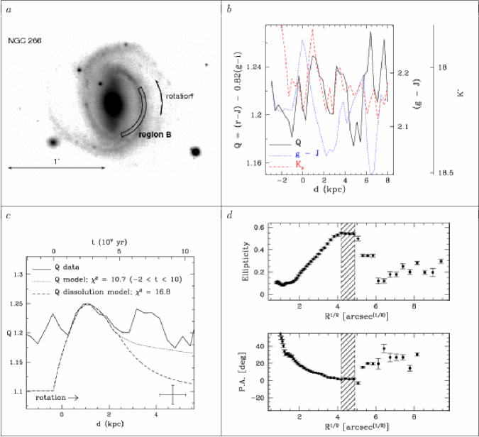
Figure 13: NGC 266, region B. (c.) Dotted and dashed lines: stellar population models, IMF $M_{\rm upper}=10M_{\sun}$.

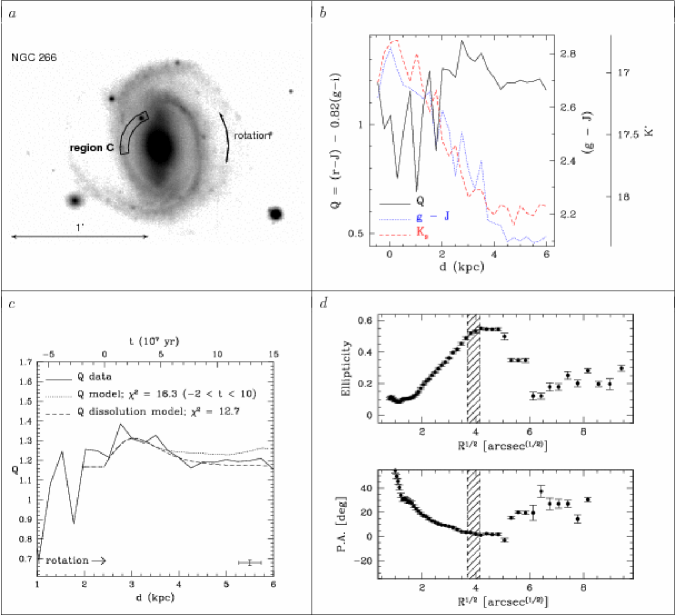
Figure 14: NGC 266, region C. (c.) Dotted and dashed lines: stellar population models, IMF $M_{\rm upper}=10M_{\sun}$.

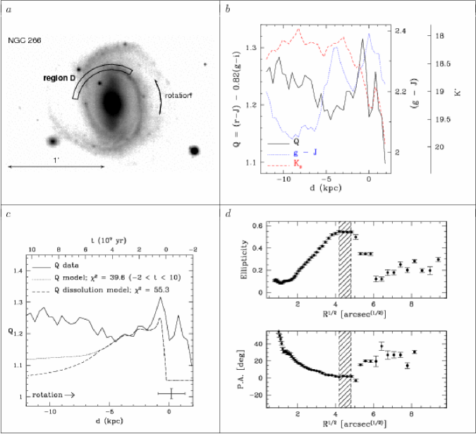
Figure 15: NGC 266, region D. (c.) Dotted and dashed lines: stellar population models, IMF $M_{\rm upper}=100M_{\sun}$.

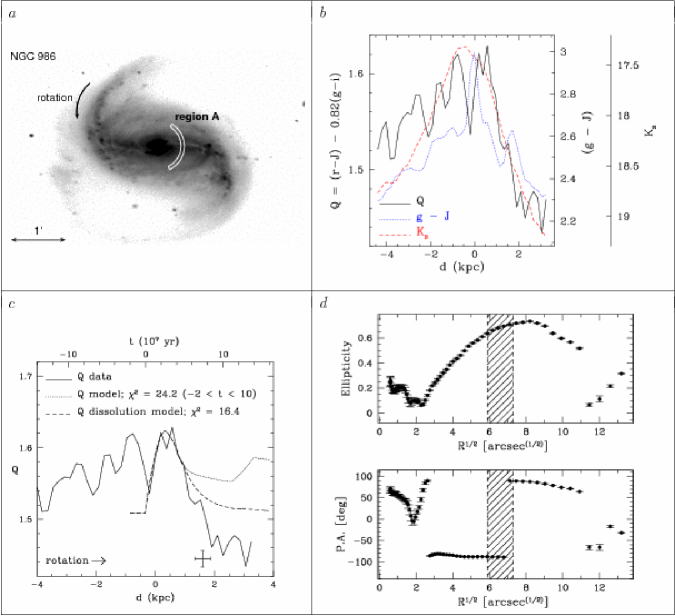
Figure 16: NGC 986, region A. (c.) Dotted and dashed lines: stellar population models, IMF $M_{\rm upper}=10M_{\sun}$.

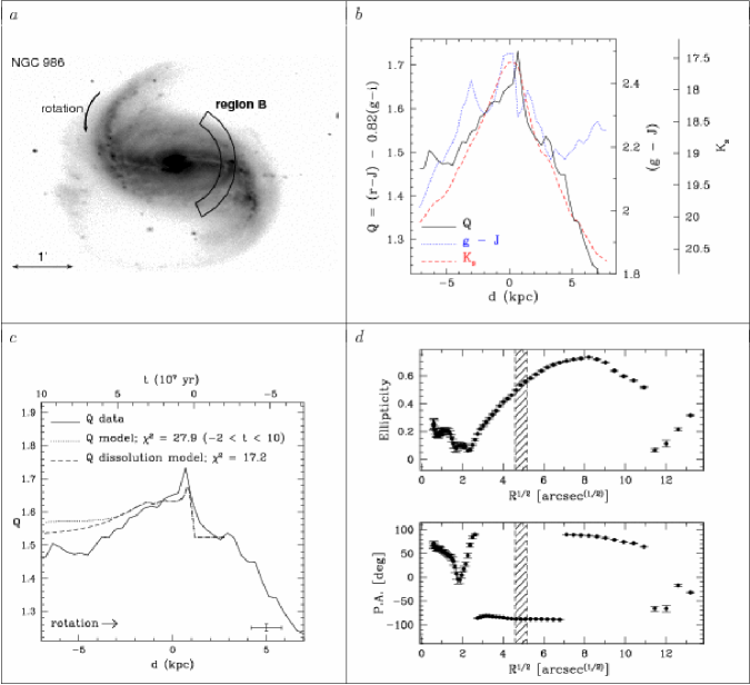
Figure 17: NGC 986, region B. (c.) Dotted and dashed lines: stellar population models, IMF $M_{\rm upper}=100M_{\sun}$.

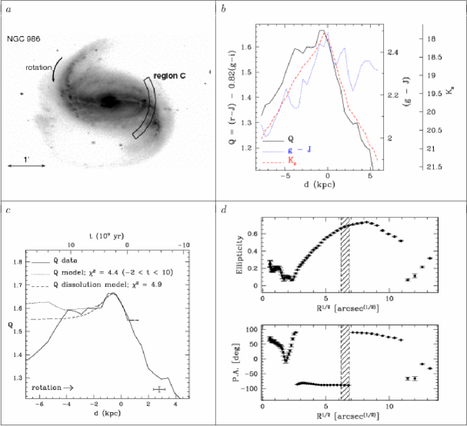
Figure 18: NGC 986, region C. (c.) Dotted and dashed lines: stellar population models, IMF $M_{\rm upper}=10M_{\sun}$.

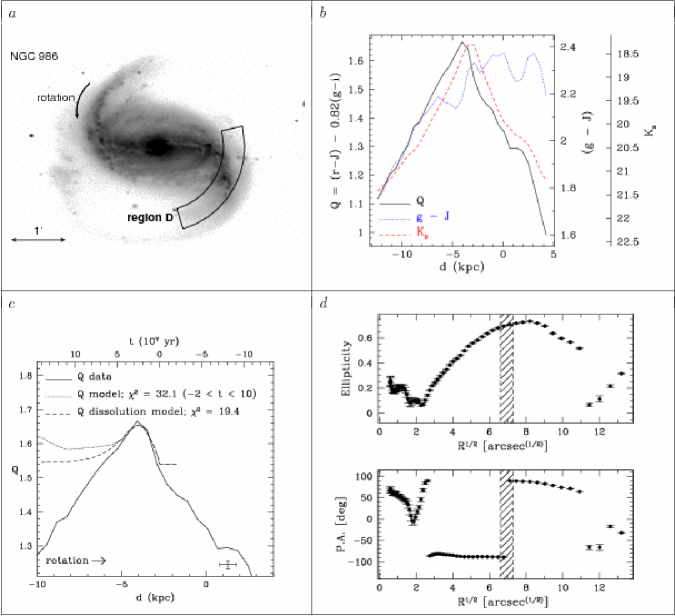
Figure 19: NGC 986, region D. (c.) Dotted and dashed lines: stellar population models, IMF $M_{\rm upper}=10M_{\sun}$.

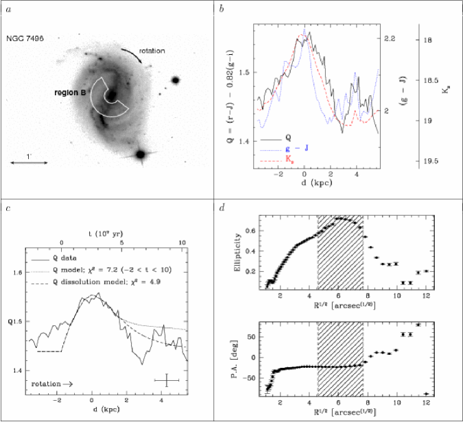
Figure 21: NGC 7496, region B. (c.) Dotted and dashed lines: stellar population models, IMF $M_{\rm upper}=10M_{\sun}$.

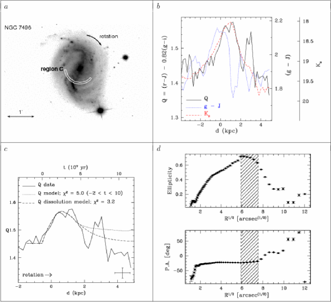
Figure 22: NGC 7496, region C. (c.) Dotted and dashed lines: stellar population models, IMF $M_{\rm upper}=10M_{\sun}$.

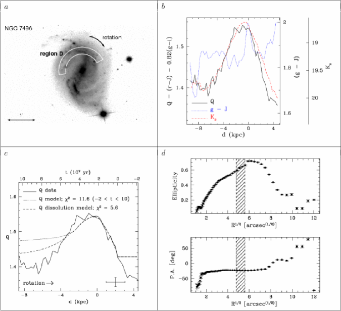
Figure 23: NGC 7496, region D. (c.) Dotted and dashed lines: stellar population models, IMF $M_{\rm upper}=10M_{\sun}$.

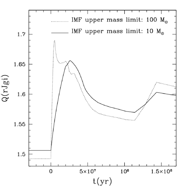
Figure 45: $Q(rJgi)$ profiles vs. time, stellar population synthesis models of S. Charlot & G. Bruzual with solar metallicity (2007, private communication), for the Lick system response curves. Dotted line: IMF upper mass limit $M_{\rm upper}=100M_{\sun}$; solid line: $M_{\rm upper}=10M_{\sun}$. A star formation burst with duration of $2\times 10^{7}$ yr was superimposed on a background population $5\times 10^{9}$ yr old. Young stars constitute 2% by mass. 

In figures 3-44, ordered by galaxy Hubble type, we show results for 42 regions with color gradient candidates. Of these, 22 are located along the bar, and 20 are found in the spiral arms. For all objects, the direction of disk rotation was established assuming that spiral arms trail. Dust lane locations were inferred from the ($g-J$) color, and bar or spiral perturbations were traced in the NIR. We fit the data with the stellar population synthesis models of S. Charlot & G. Bruzual (2007, private communication); only models with solar metallicity are considered. The duration of the star formation burst is taken to be $2\times 10^{7}$ yr; a fraction of young stars of 2% by mass is mixed with a background of old stars $5\times 10^{9}$ yr old. We use a Salpeter initial mass function (IMF) with a lower mass limit $M_{\rm lower}=0.1M_{\sun}$, and we try two different IMF upper mass limits $M_{\rm upper}$: 10 and 100 $M_{\sun}$ (see figure 45). It is important to have in mind that real data may have $M_{\rm upper}$ somewhere in between these values. Models with $M_{\rm upper}=100M_{\sun}$ exhibit a sharp peak shortly after $t_{\rm age}=0$ yr that is absent in those with $M_{\rm upper}=10M_{\sun}$. In real data this peak may be easily lost in low signal to noise regions or low resolution data, or confused with unnoticed artifacts or cosmic rays. Also, there appears to be an inverse correlation between gradient detectability and $H_{\alpha}$ emission (GG96, Martínez-García et al., 2009a), that could be explained if contamination from bright emission lines produced in HII regions around the most massive stars masks the color gradients. We are able to fit a model with $M_{\rm upper}=100M_{\sun}$ only in 7 out of 42 regions (17%).

For bar regions, we assume that stars age in the direction of rotation. In spiral regions, we search for dust lanes upstream of star formation, and (or) establish the aging direction from the“match” between the asymmetric profiles of the observations and the stellar models (see figure 45).

Each one of figures  3-44 corresponds to an analyzed region. A deprojected mosaic of the galaxy (in the $g$-band, unless otherwise indicated), in logarithmic scale, is shown in the top left panel (a). The top right panel (b) displays the observed $Q(rJgi)$ profile vs. azimuthal distance, $d$, in kpc (solid line and left y-axis); the observed ($g-J$) color vs. $d$ (dotted line and second-from-right y-axis), with high values indicating dust lane locations; and the observed $K_{s}$ surface brightness (in mag arcsec^-2, lower values correspond to higher densities of old stars) vs. $d$ (dashed line and rightmost y-axis). In the bottom left panel (c), a zoomed-in version of the $Q(rJgi)$ vs. $d$ profile (solid line) is compared with a stellar population model (dotted line) that has been “stretched” in $t_{\rm age}$ to fit the data. Model stellar age, $t_{\rm age}$, in units of $10^{7}$ yr, is shown in the upper $x$-axis. The vertical error bars show the size of photometric random errors, excluding the systematic calibration error; horizontal error bars represent possible deformations of the $Q(rJgi)$ profiles, due to density and metallicity variations in the young and old populations (see Martínez-García et al., 2009a). We also compare the data with a model that considers the dissolution of stellar groups (Wielen, 1977) after 50 Myr (dashed line, see § 5.1.1). Reduced values of

$$\chi^{2}=\Sigma\left(\frac{Q_{\rm data}-Q_{\rm model}}{\sigma_{Q(rJgi)}}\right)^{2}$$ (5)

were calculated for both models in the time interval $-20<t_{\rm age}\rm{(Myr)}<100$. The bottom right panel (d) exhibits isophote ellipticity vs. $R^{1/2}$ in the upper plot, and isophotal PA vs. $R^{1/2}$ in the lower one. Error bars were obtained from the ELLIPSE task in IRAF. Hatched regions highlight the bar corotation region, as derived from the comparison between photometric data and stellar models.

In table 4, we show the pattern speeds and resonance radii inferred from the comparison of stellar population synthesis models with observed color gradients.

Remarks for each object:

NGC 718 (Figures 3 - 5). Regions A and B belong to the bar region. For both regions, the origin ($t_{\rm age}=0$) of the stellar model that bests fits the observations is located in the leading side of the bar; the two regions yield a similar bar CR radius, within the errors. An inverse gradient is observed in spiral region NGC 718 C; this region was fit with $M_{upper}=100M_{\sun}$. The arm and bar pattern speeds are similar in this object.

NGC 864 (Figures 6 - 9). Although the positions of color gradient candidates A and B, in the bar region, are quite different, relative to the bar $K_{s}$ surface brightness and dust ($g-J$) profiles, their analysis provides a similar CR position, within the errors. This barred galaxy has spiral arms with a “ragged” structure. Region C, located in the beginning of the eastern arm (left arm in the deprojected image), gives a corotation position near the end of the spiral arms, at $\sim 76.5\pm 0.5$ arcsec. Region D, situated in an arm structure apparently decoupled from the main pattern, gives a corotation position similar to that of region C, within the errors. The two main arms of this object have different $Q$ mean values, possibly owing to different levels of star formation activity

NGC 4314 (Figures 10 - 11). Two color gradient candidates were found in the bar of this object. The one in region A is located in the leading side of the bar; the CR radius inferred from the comparison between theoretical and observed $Q(rJgi)$ profiles is near the location of maximum ellipticity. The color gradient candidate in region B is located in the trailing side of the bar; the inferred CR agrees, within the errors, with the result from region A. No color gradients were found in the arms.

NGC 266 (Figures 12 - 15). Unfortunately, the error due to the inclination angle, $\alpha$, is higher than the $\alpha$ value itself (see table 3). Although this produces very large errors in the computed $\Omega_{p}$ values, the errors in the resonance positions are reasonable, when equations A1 and A3 from Martínez-García et al. (2009a) are used. Region A is the only one detected in the bar of this object, and its analysis yields a CR position close to the maximum of isophotal ellipticity; this region was fitted with a model with $M_{\rm upper}=100M_{\sun}$. Regions B (presumably just before corotation, $M_{upper}=10M_{\sun}$) and D (presumably just after corotation, $M_{upper}=100M_{\sun}$) give similar resonance positions that also agree with the results of region A, within the errors. The resonance position derived from region C is within 1 $\sigma$ of the result of region A, and within 2 $\sigma$ of the position found from regions B and D. Regions B and C appear to be associated with a “ring” feature, rather than with the spiral arms.

NGC 986 (Figures 16 - 19). This galaxy shows an important activity in the bar region when observed in the $Q(rJgi)$ index. The bar’s end is made evident more by the change in PA of the isophotes, than by the location of their maximum ellipticity. Region A harbors a color gradient candidate in the bar whose analysis results in a CR radii close to the place where the isophotes change PA. Region B is located near the end of the bar; the fit of a stellar model (with $M_{\rm upper}=100M_{\sun}$) to its observed $Q(rJgi)$ profile gives a CR position that does not coincide with the bar’s end. For regions C and D, in one of the arms, the corotation position coincides (within the errors) with the bar’s end.

NGC 7496 (Figures 20 - 24). The northern spiral arm (lower arm in our deprojected image) displays a compact elongated region of high surface brightness, even in $K_{s}$; this arm is also more extended in radius, when compared to the southern arm (upper arm in our deprojected image). Regions A and B are located in the bar and give similar CR radii, that encompass the location of maximum ellipticity of the bar. Region C is probably located near the bar’s CR, a fact that makes the determination of dynamic parameters uncertain. The observations, and the fit of the stellar model to regions D and E indicate inverse color gradients. Corotation is close to the ellipticity maximum of the bar; all the derived positions agree within 1 $\sigma$, except for the determination from region D.

NGC 5383 (Figures 26 - 26). This barred galaxy has very short spiral arms that do not reach the outer disk. The analysis of color gradient candidates in regions A and B results in similar CR positions before the end of the bar. This may be due to strong non-circular motions that lead to an overestimate of $\Omega_{p}$, and hence to an underestimation of the CR radius.

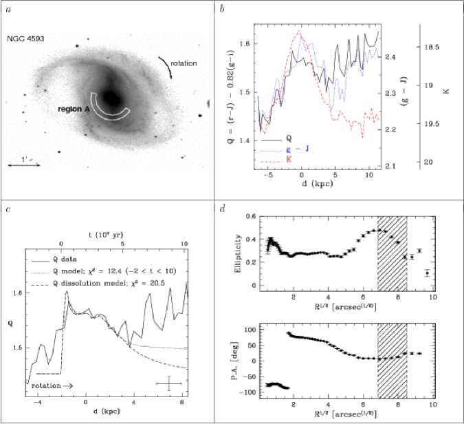
Figure 27: NGC 4593, region A. (c.) Dotted and dashed lines: stellar population models, IMF $M_{\rm upper}=100M_{\sun}$.

NGC 4593 (Figures 27 - 31). Regions A ($M_{\rm upper}=100M_{\sun}$) and B ($M_{\rm upper}=10M_{\sun}$), in the bar region, give a similar CR position near the maximum of ellipticity. Region C is located near the bar’s end, and is probably associated with a “ring” feature. Region D, inverse color gradient in the spiral arm region, gives a similar corotation position in accordance with regions A and B. Region E (“direct” color gradient) yields a corotation position further away from the galaxy center than the one inferred from region D. The eastern and western sides of the bar (respectively, upper and lower sides in the deprojected frame) have different $Q(rJgi)$ mean values.

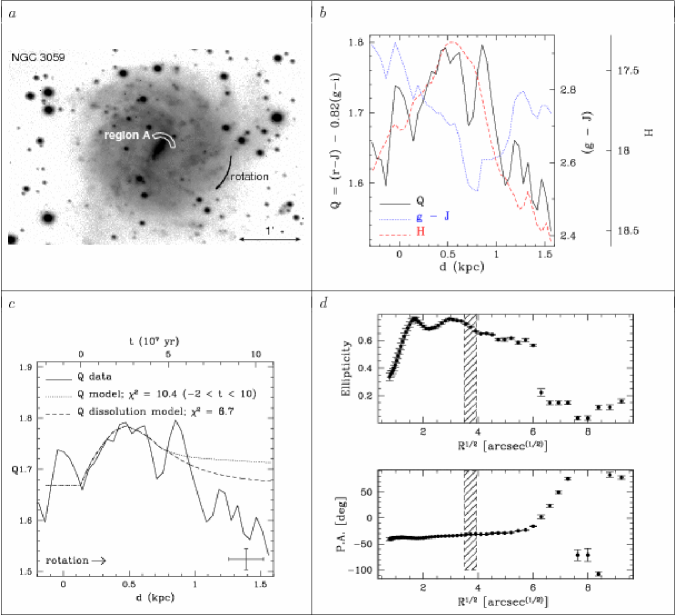
Figure 32: NGC 3059, region A. (d): isophotes from $H$-band mosaic. (c.) Dotted and dashed lines: stellar population models, IMF $M_{\rm upper}=10M_{\sun}$.  

NGC 3059 (Figures 32 - 33). This object is likely a double-bar system, and it is difficult to assess the bar’s end from the ellipticity and PA vs. radius plots. However, the CR position derived from the bar region A lies close to the bar endpoint determined from visual inspection ($\sim 19.2\pm 1.4$ arcsec). Region B in the arms, gives a corotation position at radii larger than the bar’s end.

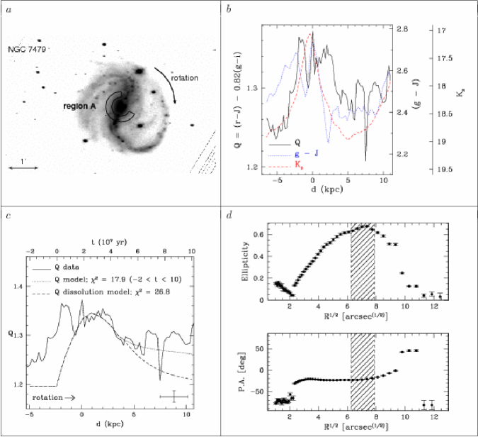
Figure 34: NGC 7479, region A. (c.) Dotted and dashed lines: stellar population models, IMF $M_{\rm upper}=10M_{\sun}$.

NGC 7479 (Figures 34 - 38). According to Wozniak et al. (1995), the HII regions located along the bar, near the dust lanes, show a “stretched” appearance probably due to strong gas flows that may trigger star formation. Regions A, B, ($M_{\rm upper}=10M_{\sun}$), and C ($M_{\rm upper}=100M_{\sun}$) show candidate color gradients in the bar. The comparison of stellar models with observations renders CR positions close to the ellipticity maximum (i.e., close to the bar’s end). Region D, situated in one of the spiral arms and after the bar’s corotation, features an inverse color gradient. The computed resonance positions agree, within the errors, for regions A through D. Region E lies near the bar’s end; even though no color gradients are expected at this position, the $Q(rJgi)$ profile indicates that some star formation is taking place.

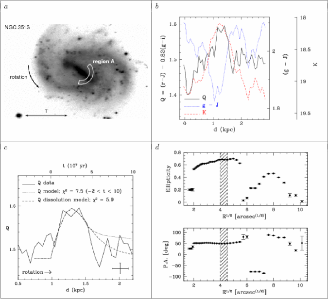
Figure 39: NGC 3513, region A. (d): isophotes from $H$-band mosaic. (c.) Dotted and dashed lines: stellar population models, IMF $M_{\rm upper}=10M_{\sun}$.  

NGC 3513 (Figures 39 - 44). Regions B, C, E, and F exhibit several adjacent $Q(rJgi)$ profiles, so it is hard to define a unique color gradient candidate. Regions A and B belong to the bar, and their analysis locates CR just inside its end. Region C is located very close to the bar’s end. Region D, in the spiral arm region, is presumably located inside corotation; the best fit of the models to the observed $Q(rJgi)$ profiles suggests $M_{\rm upper}=100M_{\sun}$ for this region, and yields a corotation radius close to the change in ellipticity and PA. In contradiction with the region D result, regions E and F indicate that the bar and spiral perturbations may rotate with different pattern speeds. Once again, $Q(rJgi)$ has different mean values in both arms.

Table 4: Observed and derived dynamic parameters.

Galaxy and region	Figure	Location	$R_{\rm mean}$ (arcsec)	$R_{\rm mean}$ (kpc)	$R_{\rm bar}$ (arcsec)	$R_{\rm bar}$ (kpc)	$\Omega_{p}$ (km s-1 kpc-1)	$R_{\rm CR}$ (arcsec)	$R_{\rm CR}$ (kpc)
NGC718 A	3	Bar	$20.7\pm 0.25$	$2.4\pm 0.2$	22.4 $\pm$ 2.0 ($K_{s}$)	2.6 $\pm$ 0.3	$37.9\pm 24.2$	$26.7\pm 5.5$	$3.1\pm 0.6$
NGC718 B	4	Bar	$21.2\pm 0.25$	$2.5\pm 0.2$	22.4 $\pm$ 2.0 ($K_{s}$)	2.6 $\pm$ 0.3	$41.4\pm 23.6$	$24.4\pm 3.6$	$2.9\pm 0.4$
NGC718 C	5	Spiral	$41.4\pm 0.25$	$4.9\pm 0.4$	22.4 $\pm$ 2.0 ($K_{s}$)	2.6 $\pm$ 0.3	$33.6\pm 13.2$	$30.1\pm 3.0$	$3.5\pm 0.4$
NGC864 A	6	Bar	$26.0\pm 0.25$	$2.8\pm 0.2$	36.1 $\pm$ 3.5 ($K_{s}$)	3.8 $\pm$ 0.5	$38.6\pm 6.5$	$36.5\pm 4.7$	$3.9\pm 0.5$
NGC864 B	7	Bar	$27.7\pm 0.25$	$3.0\pm 0.3$	36.1 $\pm$ 3.5 ($K_{s}$)	3.8 $\pm$ 0.5	$44.1\pm 6.6$	$31.9\pm 3.4$	$3.4\pm 0.4$
NGC864 C	8	Spiral	$40.4\pm 0.25$	$4.3\pm 0.4$	36.1 $\pm$ 3.5 ($K_{s}$)	3.8 $\pm$ 0.5	$18.6\pm 4.1$	$75.5\pm 13.5$	$8.1\pm 1.4$
NGC864 D	9	Spiral	$61.1\pm 0.25$	$6.5\pm 0.6$	36.1 $\pm$ 3.5 ($K_{s}$)	3.8 $\pm$ 0.5	$17.0\pm 3.1$	$82.6\pm 11.0$	$8.8\pm 1.2$
NGC4314 A	10	Bar	$44.6\pm 0.25$	$3.8\pm 0.5$	70.3 $\pm$ 17.0 ($K_{s}$)	6.0 $\pm$ 1.6	$30.6\pm 10.4$	$59.3\pm 11.0$	$5.1\pm 0.9$
NGC4314 B	11	Bar	$30.4\pm 0.25$	$2.6\pm 0.3$	70.3 $\pm$ 17.0 ($K_{s}$)	6.0 $\pm$ 1.6	$42.4\pm 15.5$	$42.8\pm 8.8$	$3.7\pm 0.8$
NGC266 A	12	Bar	$16.0\pm 0.14$	$5.0\pm 0.4$	17.5 $\pm$ 1.7 ($K^{\prime}$)	5.5 $\pm$ 0.7	$193.1\pm 452.9$	$17.0\pm 2.4$	$5.3\pm 0.8$
NGC266 B	13	Spiral	$19.6\pm 0.14$	$6.2\pm 0.5$	17.5 $\pm$ 1.7 ($K^{\prime}$)	5.5 $\pm$ 0.7	$158.3\pm 372.7$	$20.7\pm 3.3$	$6.5\pm 1.0$
NGC266 C	14	Spiral	$15.1\pm 0.14$	$4.7\pm 0.4$	17.5 $\pm$ 1.7 ($K^{\prime}$)	5.5 $\pm$ 0.7	$213.0\pm 485.6$	$15.4\pm 1.8$	$4.8\pm 0.6$
NGC266 D	15	Spiral	$22.9\pm 0.14$	$7.2\pm 0.6$	17.5 $\pm$ 1.7 ($K^{\prime}$)	5.5 $\pm$ 0.7	$158.6\pm 318.1$	$20.7\pm 2.7$	$6.5\pm 0.8$
NGC986 A	16	Bar	$26.9\pm 0.15$	$3.7\pm 0.3$	50.5 $\pm$ 4.6 ($K_{s}$)	6.8 $\pm$ 0.9	$11.2\pm 4.3$	$43.9\pm 9.2$	$6.0\pm 1.3$
NGC986 C	17	Spiral	$52.4\pm 0.15$	$7.1\pm 0.6$	50.5 $\pm$ 4.6 ($K_{s}$)	6.8 $\pm$ 0.9	$20.5\pm 2.5$	$23.8\pm 2.8$	$3.2\pm 0.4$
NGC986 D	18	Spiral	$68.9\pm 0.15$	$9.4\pm 0.8$	50.5 $\pm$ 4.6 ($K_{s}$)	6.8 $\pm$ 0.9	$11.4\pm 1.9$	$42.8\pm 4.0$	$5.8\pm 0.5$
NGC986 E	19	Spiral	$83.7\pm 0.15$	$11.4\pm 1.0$	50.5 $\pm$ 4.6 ($K_{s}$)	6.8 $\pm$ 0.9	$10.1\pm 1.6$	$48.2\pm 4.7$	$6.5\pm 0.6$
NGC7496 A	20	Bar	$21.5\pm 0.15$	$2.5\pm 0.2$	38.0 $\pm$ 3.5 ($K_{s}$)	4.3 $\pm$ 0.5	$39.6\pm 32.5$	$35.0\pm 14.4$	$4.0\pm 1.6$
NGC7496 B	21	Bar	$23.0\pm 0.15$	$2.6\pm 0.2$	38.0 $\pm$ 3.5 ($K_{s}$)	4.3 $\pm$ 0.5	$34.6\pm 30.2$	$40.1\pm 18.9$	$4.6\pm 2.2$
NGC7496 C	22	Bar	$33.0\pm 0.15$	$3.8\pm 0.3$	38.0 $\pm$ 3.5 ($K_{s}$)	4.3 $\pm$ 0.5	$30.1\pm 20.2$	$46.0\pm 11.2$	$5.3\pm 1.3$
NGC7496 D	23	Spiral	$44.1\pm 0.15$	$5.0\pm 0.4$	38.0 $\pm$ 3.5 ($K_{s}$)	4.3 $\pm$ 0.5	$51.4\pm 13.8$	$27.0\pm 4.2$	$3.1\pm 0.5$
NGC7496 E	24	Spiral	$68.4\pm 0.15$	$7.8\pm 0.7$	38.0 $\pm$ 3.5 ($K_{s}$)	4.3 $\pm$ 0.5	$31.1\pm 9.3$	$44.6\pm 5.9$	$5.1\pm 0.7$
NGC5383 A	25	Bar	$20.1\pm 0.25$	$3.8\pm 0.3$	54.2 $\pm$ 5.0 ($K_{s}$)	10.3 $\pm$ 1.3	$65.2\pm 19$	$21.9\pm 2.4$	$4.2\pm 0.5$
NGC5383 B	26	Bar	$27.3\pm 0.25$	$5.2\pm 0.5$	54.2 $\pm$ 5.0 ($K_{s}$)	10.3 $\pm$ 1.3	$48.8\pm 13.6$	$29.2\pm 3.0$	$5.6\pm 0.6$
NGC4593 A	27	Bar	$34.8\pm 0.14$	$6.4\pm 0.6$	48.0 $\pm$ 4.4 ($K$)	8.9 $\pm$ 1.1	$21.8\pm 6.4$	$59.5\pm 12.9$	$11.0\pm 2.4$
NGC4593 B	28	Bar	$36.7\pm 0.14$	$6.8\pm 0.6$	48.0 $\pm$ 4.4 ($K$)	8.9 $\pm$ 1.1	$26.8\pm 5.6$	$48.5\pm 6.6$	$9.0\pm 1.2$
NGC4593 C	29	Spiral	$56.1\pm 0.14$	$10.4\pm 0.9$	48.0 $\pm$ 4.4 ($K$)	8.9 $\pm$ 1.1	$10.3\pm 4.1$	$125.8\pm 41.4$	$23.3\pm 7.7$
NGC4593 D	30	Spiral	$72.6\pm 0.14$	$13.4\pm 1.2$	48.0 $\pm$ 4.4 ($K$)	8.9 $\pm$ 1.1	$27.0\pm 2.8$	$48.1\pm 3.0$	$8.9\pm 0.6$
NGC4593 E	31	Spiral	$64.1\pm 0.14$	$11.9\pm 1.0$	48.0 $\pm$ 4.4 ($K$)	8.9 $\pm$ 1.1	$11.1\pm 3.3$	$117.0\pm 25.7$	$21.7\pm 4.8$
NGC3059 A	32	Bar	$12.4\pm 0.14$	$0.9\pm 0.1$	19.2 $\pm$ 1.4 ($H$)	1.4 $\pm$ 0.2	$121.2\pm 49.8$	$13.9\pm 1.6$	$1.0\pm 0.1$
NGC3059 B	33	Spiral	$26.5\pm 0.14$	$1.9\pm 0.2$	19.2 $\pm$ 1.4 ($H$)	1.4 $\pm$ 0.2	$58.6\pm 23.6$	$28.7\pm 3.1$	$2.1\pm 0.2$
NGC7479 A	34	Bar	$25.0\pm 0.25$	$4.2\pm 0.4$	54.2 $\pm$ 5.0 ($K_{s}$)	9.0 $\pm$ 1.1	$29.5\pm 8.1$	$50.5\pm 11.3$	$8.4\pm 1.9$
NGC7479 B	35	Bar	$47.6\pm 0.25$	$7.9\pm 0.7$	54.2 $\pm$ 5.0 ($K_{s}$)	9.0 $\pm$ 1.1	$19.8\pm 4.3$	$75.2\pm 12.3$	$12.5\pm 2.1$
NGC7479 C	36	Bar	$41.4\pm 0.25$	$6.9\pm 0.6$	54.2 $\pm$ 5.0 ($K_{s}$)	9.0 $\pm$ 1.1	$21.9\pm 4.8$	$68.2\pm 11.6$	$11.4\pm 1.9$
NGC7479 D	37	Spiral	$80.3\pm 0.25$	$13.4\pm 1.1$	54.2 $\pm$ 5.0 ($K_{s}$)	9.0 $\pm$ 1.1	$27.5\pm 2.2$	$54.2\pm 3.3$	$9.0\pm 0.6$
NGC7479 E	38	Spiral	$60.1\pm 0.25$	$10.0\pm 0.8$	54.2 $\pm$ 5.0 ($K_{s}$)	9.0 $\pm$ 1.1	$14.4\pm 3.4$	$103.7\pm 19.1$	$17.3\pm 3.2$
NGC3513 A	39	Bar	$14.8\pm 0.14$	$1.1\pm 0.1$	24.6 $\pm$ 2.5 ($H$)	1.9 $\pm$ 0.3	$45.0\pm 10.1$	$18.2\pm 2.2$	$1.4\pm 0.2$
NGC3513 B	40	Bar	$17.0\pm 0.14$	$1.3\pm 0.1$	24.6 $\pm$ 2.5 ($H$)	1.9 $\pm$ 0.3	$39.5\pm 8.9$	$20.7\pm 2.5$	$1.6\pm 0.2$
NGC3513 C	41	Bar	$24.1\pm 0.14$	$1.9\pm 0.2$	24.6 $\pm$ 2.5 ($H$)	1.9 $\pm$ 0.3	$28.2\pm 6.1$	$29.0\pm 3.4$	$2.3\pm 0.3$
NGC3513 D	42	Spiral	$20.8\pm 0.14$	$1.6\pm 0.1$	24.6 $\pm$ 2.5 ($H$)	1.9 $\pm$ 0.3	$22.9\pm 7.3$	$35.8\pm 7.5$	$2.8\pm 0.6$
NGC3513 E	43	Spiral	$43.0\pm 0.14$	$3.3\pm 0.3$	24.6 $\pm$ 2.5 ($H$)	1.9 $\pm$ 0.3	$9.9\pm 3.7$	$82.7\pm 19.8$	$6.4\pm 1.5$
NGC3513 F	44	Spiral	$35.8\pm 0.14$	$2.8\pm 0.2$	24.6 $\pm$ 2.5 ($H$)	1.9 $\pm$ 0.3	$14.7\pm 4.2$	$55.6\pm 9.8$	$4.3\pm 0.8$

Note. — Col. (4) and (5). Mean radius of the studied regions, in arcsec and kpc, respectively. Col. (6) and (7). Radius of the bar, in arcsec and kpc, respectively, and bandpass used to determine it. Col. (8) Pattern speed. Col. (9) and (10). Corotation radius, in arcsec and kpc, respectively.

5 Discussion

5.1 Characteristics of observed color gradients

In a “standard color gradient picture”, assuming circular motions, one would expect an azimuthal sequence starting with compression of gas, dust lanes, star formation onset and stellar drift, which would lead to color gradients. When one adds an extended period of star formation, dispersion velocities and post shock velocities, the predicted color profiles may become rather broad (see, e.g., Yuan & Grosbol, 1981).

Although shocks and/or dust lanes are located mainly upstream relative to the spiral potential minimum, in a more detailed scenario, for certain models and relatively short radial intervals, they can be found downstream (in the gas stream direction) the spiral potential minimum (Gittins & Clarke, 2004). This is due to the fact that pitch angles of the arms are expected to follow $i_{\mathrm{P}}>i_{\mathrm{D}}>i_{\mathrm{SF}}$, where $i_{\mathrm{P}}$ is the pitch angle of the potential, $i_{\mathrm{D}}$ is the pitch angle of the dust lane (the shock), and $i_{\mathrm{SF}}$ is the pitch angle of star formation. According to this, the azimuthal relative location of potential and dust lanes may change within the same galaxy and be radially dependent. In principle, the local potential minimum could be determined from the the $K$-band spiral arm. Nevertheless, gravity is a long-range force, and all the non-axisymmetric contributions must be taken into account for local potential minimum determinations. Thus, the local potential does not necessarily coincide with the local density of old stars (see, e.g., Zhang, 1996; Berman, 2003; Gittins & Clarke, 2004; Zhang & Buta, 2007; Buta & Zhang, 2009), and the expected locations of the dust lanes must follow the potential, rather than the $K$-band intensity.

For some of the bar regions presented in figures 3-44, the $t_{\rm age}=0$ location of the gradient seems to be located before the main dust lane peak. This can be attributed to the fact that star formation in bars is supposed to begin at the dust “spurs” of the bar itself (see § 1.1), which are located in the “trailing” side and upstream the main dust lanes.

For this investigation the $d=0$ distance (i.e., the assumed shock location) is chosen where the maximum in the $g-J$ color is observed. This is the case, even for regions where double peaks or dust lanes are seen (e.g., region NGC 864 B, figure 7). For most of the fits we do not have $t_{\rm age}=0$ for $d=0$ precisely (e.g., region NGC 7496 A in figure 20). This is due to the fact that only the width of the model profile in $Q(rJgi)$ is fitted to the observations by stretching. Theoretically, for spiral regions $t_{\rm age}=0$ should coincide or be located after $d=0$. In real galaxies, it is hard to pinpoint where the onset of star formation really occurs. One important reason is the fact that a diffuse cloud of neutral gas has first to become a dense cloud, then a molecular cloud, and finally a self-gravitating cloud to achieve star formation; this process may take $∼\sim 10^{7}$ years (see, e.g., Tamburro et al., 2008; Egusa et al., 2009).

5.1.1 Downstream decline of the gradients

Martínez-García et al. (2009a) already noticed that for some spiral regions there is a “downstream decline” (or “downstream fall”) of the gradients. In such regions, the observed $Q(rJgi)$ profile declines below the model (or the value $Q(rJgi)\sim 1.57$, for solar metallicity, in figure 45), apparently returning to the “old background population” level, or lower, by $t\approx 5\times 10^{7}$ years, much faster than the theoretical expectations. This is the case, for example, of regions NGC 864 C, NGC 7496 B & C, NGC 7479 B, NGC 3513 A & C (figures 8, 21, 22, 35, 39, and 41, respectively), for which the fit between $Q(rJgi)$ data and dotted line model is not good, except for the range $0\lesssim t_{\rm age}\lesssim 50$ Myr.

Martínez-García et al. (2009a) hypothesized that the decline of the observed $Q(rJgi)$ profiles below the models (that assume pure circular orbits) might be caused by stellar non-circular motions in the data. However, Martínez-García et al. (2009b) found that non-circular motions cannot explain the discrepancy.

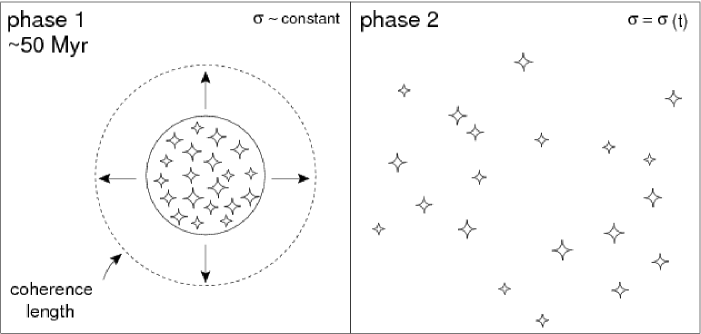
Figure 46: Dissolution of stellar groups scenario (Wielen, 1977). During phase 1 ($\sim$ 50 Myr), the stellar group increases its diameter due to a $\sim$ constant internal velocity dispersion, until the “coherence length” is reached. During phase 2, the velocity dispersion increases with time and the “diffusion of stellar orbits” causes the dissipation of the stellar group.

A solution to this problem may be provided by the dissolution of stellar groups scenario proposed by Wielen (1977, see figure 46). According to this author, the diffusion of stellar orbits can enhance the dissolution of young stellar groups by increasing their internal velocity dispersion. To explain the observed increase in the velocity dispersion of stars with age, Wielen (1977) proposes the existence of local fluctuations of the gravitational field with a rather stochastic behavior. This irregular field has the effect of creating a diffusion process in the velocity space of stars. The dissolution of stellar groups proceeds in two phases. During the first phase, the internal velocity dispersion, $\sigma_{\rm int}$, causes the group to expand, until its diameter, $D_{\rm sg}(t_{\rm age})$ is larger than the distance over which simultaneous perturbations (for stars close together in space) are significantly correlated, i.e., the coherence length, $L_{\rm co}$. During this first phase, the center of mass of the group is affected by diffusion mechanisms, while the members of the group only suffer small tidal effects, thus $\sigma_{\rm int}\sim$ constant. The duration of the first phase is given by:

$$t_{\rm phase1}=0.975(L_{\rm co}-D_{\rm sg}(0))/\sigma_{\rm int},$$ (6)

for $t_{\rm phase1}$ in Myr, $L_{\rm co}-D_{\rm sg}(0)$ in pc, and $\sigma_{\rm int}$ in km s^-1. For typical values of $\sigma_{\rm int}=$10 km s^-1, and $L_{\rm co}-D_{\rm sg}(0)$=500 pc (Wielen, 1977), we have that:

$$t_{\rm phase1}\sim 50\rm{Myr}.$$

During the second phase of the dissolution (after $t_{\rm phase1}$ years), the perturbations over each star member of the group are not longer correlated, and the group dissolves with time because of the diffusion mechanism. During this phase the velocity dispersion increases with time, i.e., $\sigma=\sigma(t)$, where $t=t_{\rm age}-t_{\rm phase1}$.

In order to evaluate the relevance of the dissolution of stellar groups scenario (Wielen, 1977) for the color gradient picture, we have built a “toy model” for $Q(rJgi)$, consisting of two phases. During the first phase, while $t_{\rm age}<50$ Myr, the fractions by mass of young, $\beta_{\rm I}=2\%$, and old, $\beta_{\rm II}=98\%$, stars are kept constant. During the second phase, we assume (1) that the fraction of young stars changes as $\beta_{\rm I}\propto 1/t^{3}_{\rm age}$, and (2) that the surface density of young stars behaves in the same way (see eq. 10 in Wielen, 1977).

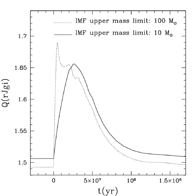
Figure 47: Same as figure 45, including dissolution of stellar groups (Wielen, 1977) after 50 Myr (see § 5.1.1).  

The models produced with this approximation are displayed in figure 47, with a continuous line for models with the IMF $M_{\rm upper}=10M_{\sun}$, and a dotted line for those with $M_{\rm upper}=100M_{\sun}$ (see also figures 8 and 9 in Martínez-García et al., 2009a). According to figure 47, the dissolution of stellar groups, as a consequence of disk heating, may provide an efficient mechanism to explain the observed “downstream decline” of the gradients encountered in Martínez-García et al. (2009a), and in this investigation. It is important to mention that the dissolution effect operates also in the presence of non-circular motions.

Other dissolution scenarios:

Another effective disruption mechanism for star clusters comes from stellar winds and supernovae explosions that remove gas (and dust) on short timescales. These perturb the potential and cause young star clusters to become unbound (see, e.g., Bastian & Goodwin, 2006; Gieles & Bastian, 2008; Lamers et al., 2005). This “infant mortality” occurs during the first 10 Myr and affects the most luminous clusters (those with the most rapid color evolution). Nevertheless, stars escape with the initial velocity dispersion of the cluster and are physically associated with it for 10-40 Myr after gas removal (Bastian & Goodwin, 2006). The color gradients presented in this investigation are probably formed by clusters that survive “infant mortality” at least for 50 Myr.

5.1.2 Color gradients in dusty environments

One more issue in the “standard color gradient picture” relates to the $Q(rJgi)$ value expected for the old background population at $t_{\rm age}<0$. Also, $Q(rJgi)$ (or any color) should return to the background value on both sides of the bar, at the same spatial offsets. In some of the observed color gradient candidates in this investigation, the $Q(rJgi)$ index does not agree well with the models for $t_{\rm age}<0$ (see, e.g., regions NGC 718 C, NGC 986 A, NGC 7479 A; figures 5, 16, and 34, respectively).

Models with pure old background population have an approximately constant $Q(rJgi)$ value, regardless of surface brightness. However, the exact value depends on the average age and metallicity of the local region (see Martínez-García et al., 2009a), that cannot, especially metallicity, be determined unambiguously just from photometric data. A complementary possible explanation of why, for some regions, the $Q(rJgi)$ index does not decline to the background value for $t_{\rm age}<0$ is that the adopted method (see § 3.1) involves averaging over radial annuli to increase the S/N ratio. Albeit we do so carefully, we may be combining zones with somewhat different background levels.

Yet another recurring concern is whether dust can mimic the $Q$ profile of a star formation burst, since $Q(rJgi)$ is reddening-insensitive for a foreground screen, but not exactly so for a mixture of dust and stars (González & Graham, 1996; Martínez-García et al., 2009a). The main expected effect would be a higher $Q(rJgi)$ value (see figure 48).

Assuming $\tau_{V}\sim 1.0$ (e.g., Xilouris et al., 1999) for a nearly face-on disk, given the inclination angles of the galaxy sample, our observations cover on average the range $0<\tau_{V}<2.0$. For regions where $t_{\rm age}<0$, though, thick dust lanes may be present with $\tau_{V}~{}\gg~{}2.0$.

From the Charlot & Fall (2000, see also Bruzual & Charlot 2003) dust model, we get the linear relation $Q(rJgi)=0.02\tau_{V}+1.51$ (where 1.51 is the background $Q(rJgi)$ value; see figure 48 for $t_{\rm age}\sim 0$). Thus, to get a $Q(rJgi)$ profile reminiscent of a density wave induced color gradient in the absence of young stars, with a peak value $\sim 1.66$, the dust must have $\tau_{V}\sim 7.0$. But also, for this scenario to take place, $\tau_{V}$ must increase for $Q(rJgi)$ to increase, and viceversa, i.e., the profile in a reddening sensitive index, like ($g-J$), must follow the $Q(rJgi)$ azimuthal distribution.

For $t_{\rm age}>0$, dust becomes progressively less important, because star formation processes (e.g., UV radiation) sweep away and destroy available material. Indeed, concentrations of dust that are higher downstream the shock than at the shock are not observed in most real spiral arms. Fittingly, all of the observed color gradients indicate an inverse correlation between $Q(rJgi)$ and $(g-J)$, so that dust cannot be mimicking a star formation burst. Although the situation may be different for bar regions, we do not observe a correlation between the dust and $Q(rJgi)$ profiles in any of the bar gradient candidates analyzed in this investigation.

Finally, because of the connection between the gradients (i.e., star formation) and disk dynamics (i.e., the orbital resonance positions; see § 5.2), we argue that dust features are not affecting the analyzed gradients in any important way.

5.2 Connection with dynamics

In figure 49, the pattern speed obtained from each region in NGC 7479 is plotted vs. the mean radius of the region. Notice the tendency to derive slower $\Omega_{p}^{\rm bar}$ from bar regions (A, B, C) at larger radius. Likewise, figure 50 shows the $\Omega_{p}^{\rm bar}$ obtained for NGC 3513, vs. the radius of each region. As in plot 49 (NGC 7479), a trend whereby $\Omega_{p}^{\rm bar}\propto r^{-1}$ is observed for the bar regions (A, B, and C). In Martínez-García et al. (2009b), we found that this effect is observed in non-barred or weakly barred galaxies, if non-circular motions are present but color gradient data are analyzed assuming stars have purely circular orbits. In the case of barred galaxies, non-circular motions in the bar cause $\Omega_{p}^{\rm bar}$ to be overestimated inside the bar CR radius; once more, the size of the discrepancy between the real and the measured pattern speed increases as the radius decreases. This signature does not mean that $\Omega_{p}^{\rm bar}$ is changing with radius, in either kind of galaxy.

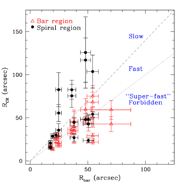
Figure 51: $R_{\rm{CR}}$ vs. $R_{\rm{bar}}$. Red open triangles: bar regions; black solid circles: spiral regions. Dotted line: $R_{\rm{CR}}=R_{\rm{bar}}$; dashed line: $R_{\rm{CR}}=1.4R_{\rm{bar}}$. Lines separate zones inhabited by “slow”, “fast” and “forbidden”  (or “super-fast”, Buta & Zhang, 2009) bars (Aguerri et al., 2003). 

Given that many of the computed resonance positions seem to be in accordance with theoretical predictions (e.g., bars ending near their CR radius), most of the analyzed color gradient candidates may indeed have a relation with the dynamics of the disk. Figure 51 shows a plot of bar extent, $R_{\rm{bar}}$ (see § 3.2), vs. bar CR radius, $R_{\rm{CR}}$, as inferred from the comparison between stellar population models, and broad-band optical and NIR observations. Red open triangles denote bar regions, whereas black solid circles indicate color gradient candidates in the arms. The plot is divided in three zones, i.e., the “slow”, “fast”, and “forbidden” bar areas; the latter corresponds to the “super-fast” bars of Buta & Zhang (2009). The dotted line, $R_{\rm{CR}}=R_{\rm{bar}}$, and the dashed line, $R_{\rm{CR}}=1.4R_{\rm{bar}}$, enclose the parameter space where most of the points should be if bars end near CR (Aguerri et al., 2003). If the spiral pattern speed, $\Omega_{p}^{\rm{spiral}}$, is similar to the bar’s pattern speed, $\Omega_{p}^{\rm{bar}}$, then spiral region points should fall in this area, too. Unfortunately, with the GG96 method it is difficult to distinguish between “super-fast” bars and the expected overestimation of $\Omega_{p}^{\rm{bar}}$, owing to non-circular motions (Martínez-García et al., 2009b). All the points below the $R_{\rm{CR}}=R_{\rm{bar}}$ (dotted) line are more likely due to the latter effect. In order to discriminate between these two possibilities, we follow Martínez-García et al. (2009b) and define:

$$\delta\Omega_{p}=\frac{\Omega_{\mathrm{data}}}{\Omega_{p}^{\prime}}-1.$$ (7)

Here, $\Omega_{\mathrm{data}}$ is the pattern speed value obtained with the GG96 method (either for the bar or the spiral), and $\Omega_{p}^{\prime}$ is the pattern speed of the (bar of spiral) perturbation derived from the rotation curve once a resonance position is fixed.

For barred spirals, in the case where bar and arms share the same pattern speed (and thus the same CR radius), we have:

$$\Omega_{p}^{\prime}\sim\frac{v_{\mathrm{rot}}}{1.2R_{\rm{bar}}},$$ (8)

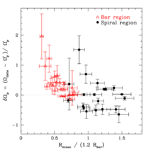
Figure 52: $\delta\Omega_{p}$ (see text) vs. $R_{\rm{mean}}/1.2R_{\rm{bar}}$. Red open triangles: bar regions; black solid circles: spiral regions. Dotted line: $\delta\Omega_{p}=0$, i.e., the pattern speed inferred from the color gradient candidates, $\Omega_{\mathrm{data}}$, equals the pattern speed derived from a flat rotation curve, if the bar CR is located at 1.2 $R_{\rm{bar}}$ (the bar end point). 

where we adopt $\frac{R_{\rm{CR}}}{R_{\rm{bar}}}\sim 1.2$, the expected ratio for spirals with well defined bars (see, e.g., Athanassoula, 1992; Elmegreen, 1996; Buta & Zhang, 2009). In figure 52, we show $\delta\Omega_{p}$ vs. $R_{\rm{mean}}/1.2R_{\rm{bar}}$; this ratio is $\sim 1$ for regions near CR. Once again, bar regions are shown with open red triangles to distinguish them from spiral regions (solid black circles). For the bar regions, there is a systematic trend, whereby $\Omega_{p}^{\rm{bar}}$ is overestimated at small radii, the magnitude of the bias is inversely correlated with radius, and the points converge to $\delta\Omega_{p}=0$ as they approach the corotation zone. This is the expected effect when non-circular motions are present, but color gradients are interpreted with a dynamic model that considers purely circular motions (Martínez-García et al., 2009b). However, as a consequence of data processing that was already discerned by these authors, regions in the outer half of the bar yield $\Omega_{p}^{\rm{bar}}$ values with less than 50% error. The detectable trend, on the other hand, confirms the link of the gradients to disk dynamics.

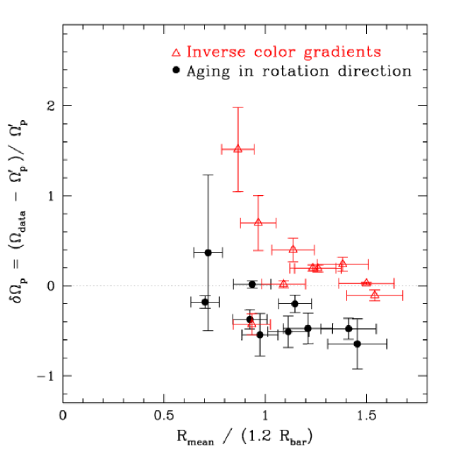
Figure 53: Same as figure 52, for the spiral regions only. Red open triangles: “inverse” color gradients; black solid circles: stellar aging and disk rotation have the same direction.

In figure 53, we plot $\delta\Omega_{p}$ for the spiral arm regions vs. region radius, in the same units as figure 52; we highlight those with “inverse” color gradients (i.e., the sense of rotation is opposite to the observed aging of stars) with open red triangles. Most of these regions lie over the dotted line, where the pattern speed obtained from the color gradient candidates, $\Omega_{\rm data}$, equals the pattern speed derived from a flat rotation curve, if the bar CR is located at 1.2 $R_{\rm bar}$. Conversely, regions where stars age in the direction of disk rotation (solid black circles) sit below the dotted line. If such “inverse” color gradients occur in objects where $\Omega_{p}^{\rm{bar}}\approx\Omega_{p}^{\rm{spiral}}$, then this plot may indicate the presence of non-circular motions close to corotation, that cause the overestimation of the pattern speed with our method.

On the other hand, the existence of gradients where stellar aging follows disk rotation, at radii beyond the bar CR radius, may be interpreted as $\Omega_{p}^{\rm{bar}}\neq\Omega_{p}^{\rm{spiral}}$, i.e., decoupled pattern speeds for the bar and the spiral; the CR radius of the spiral pattern would be larger than that of the bar.

5.3 The origin of spiral arms.

The origin of spiral arms may be different in barred galaxies than in non-barred or weakly-barred spirals. An alternative theory to density waves propounds that manifold-driven chaotic orbits are the foundation of spirals and rings (nuclear rings excluded) in barred galaxies (Patsis, 2006; Romero-Gómez et al., 2006, 2007; Athanassoula et al., 2009a, b, 2010; Voglis et al., 2006a, b; Tsoutsis et al., 2008, 2009; Harsoula & Kalapotharakos, 2009). In the view of Romero-Gómez et al. (2006, 2007) and Athanassoula et al. (2009a, b, 2010), invariant manifolds are “tubes” that guide orbits; they are associated with unstable Lagrangian points at corotation. Material is trapped in the manifolds during disk evolution, and circulates across the disk, inducing radial mixing (Athanassoula et al., 2010). Another interpretation of the “invariant manifold theory” considers only apsidal (apocentric or pericentric) sections of unstable manifolds (Voglis et al., 2006a, b; Tsoutsis et al., 2008, 2009). In this latter version, there is no need for constantly supplying material inside the manifolds (Efthymiopoulos, C., 2010).

One important prediction of the “manifold theories” (both views) is that the spiral arms and the bar must have the same pattern speed. According to the age gradients found in the spiral arms of our sample, the objects NGC 718, NGC 266, NGC 986, NGC 7496, NGC 4593, and NGC 7479 are the most likely to have $\Omega_{p}^{\rm{bar}}\approx\Omega_{p}^{\rm{spiral}}$. Conversely, NGC 864, NGC 3059, and NGC 3513 appear to have different spiral and bar pattern speeds. No conclusion can be drawn for NGC 4314 and NGC 5383, since we were able to detect gradients only in the bars of these objects. Quite interestingly, with the exception of NGC 7479, all objects in our sample with $\Omega_{p}^{\rm{bar}}\approx\Omega_{p}^{\rm{spiral}}$ are early Hubble types, while the objects with $\Omega_{p}^{\rm{bar}}\neq\Omega_{p}^{\rm{spiral}}$ are late Hubble types.

Both the density wave and the “manifold” theories predict a spiral potential that can produce shocks in the circulating gas. If star formation is triggered by these shocks, it would be difficult to discriminate between the two theories on the basis of the presence of color gradients alone. But, at least in the three objects in our sample with uncoupled bar and spiral pattern speeds, the origin of the arms and/or their subsequent evolution may follow different paths from the ones proposed by the “manifold” theory.

Concerning a different but related aspect, the observed trends for color gradients with radius in figure 53 suggest that non-circular motions are important near the bar corotation in barred galaxies, and that their effect on the determination of the spiral pattern speed are significantly stronger for inverse color gradients, i.e., when $\Omega_{p}^{\rm{bar}}\approx\Omega_{p}^{\rm{spiral}}$. The presence of non-circular motions is not surprising, given the existence of the bar. If, however, the size of $\delta\Omega_{\rm p}$ in barred galaxies correlates with shock strength, the amplitudes of coupled spiral arms should also be stronger near CR  (see, e.g., NGC 1566 spiral Fourier amplitudes in Salo et al., 2010). Strong shocks are neither expected nor observed (e.g., Martínez-García et al., 2009b) near the pattern CR radius of non-barred or weakly-barred spiral galaxies.

After a re-analysis of the result in Buta et al. (2009), who find only a weak indication that some strong bars may drive strong spirals, Salo et al. (2010) conclude, contrariwise, that in a statistical sense spiral density waves may indeed be driven by bars. More comparisons with observations (see, e.g., Grouchy et al., 2010) are needed to test both the “manifold” and the density wave theories (Athanassoula et al., 2010).

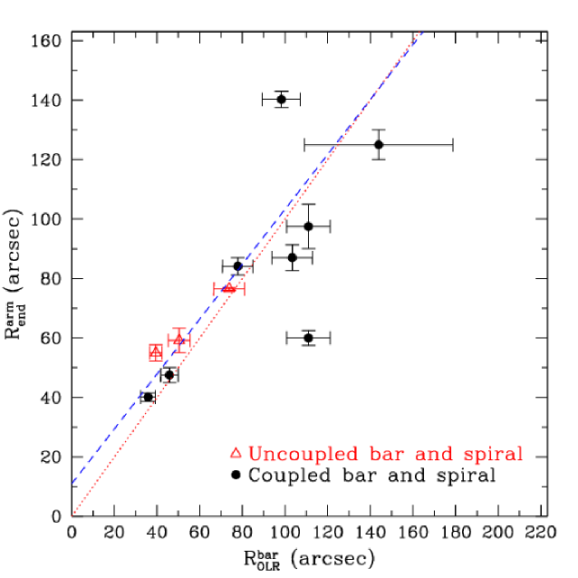
Figure 54: Mean arm maximum extent, $R^{\rm arm}_{\rm end}$, obtained by eye from NIR data, vs. bar OLR, $R^{\rm bar}_{\rm OLR}$, assuming $R_{\rm CR}=1.2R_{\rm bar}$. Red open triangles: $\Omega^{\rm bar}_{p}\neq\Omega^{\rm arm}_{p}$; black solid circles: $\Omega^{\rm bar}_{p}\approx\Omega^{\rm arm}_{p}$. Dotted line: $R^{\rm arm}_{\rm end}=R^{\rm bar}_{\rm OLR}$; dashed line: OLS (weighted by errors) bisector line.

To confirm the link between the gradients and the disk dynamics, it is also important to compare the location of the spiral “end points” with the orbital resonance positions. Schwarz (1985) shows that bar-induced gas spiral arms may reach beyond the outer Lindblad resonance (OLR) of the bar. In figure 54 we plot the OLR of the bar, $R^{\rm bar}_{\rm OLR}$, assuming

$$R^{\rm bar}_{\rm OLR}\sim 1.2R_{\rm bar}\left(1+\frac{\sqrt{2}}{2}\right),$$ (9)

vs. the spiral extent, $R_{\rm end}^{\rm arm}$, estimated by eye in the NIR, for all objects in our sample (arms with decoupled pattern speeds are shown as red open triangles). $R_{\rm end}^{\rm arm}$ values are listed in table 5.

The dotted line indicates the identity, $R_{\rm end}^{\rm arm}=R^{\rm bar}_{\rm OLR}$, while the dashed line is the OLS (ordinary least squares) bisector. On average, for our whole barred spiral galaxy sample, the radial extent of the spiral arms coincides with the OLR of the bar, regardless of the pattern speeds. Interestingly, a separate fit to the 3 decoupled spirals yields a bad match to all the end point locations expected from theory, that is, to the bar OLR, the arm CR, and the arm OLR. Since 2 of the objects (NGC 864 and NGC 3513), though, are consistent with ending at the arm CR, more data are needed to better understand the dynamics of spirals decoupled from the bar.

Table 5: Spiral maximum extents 

Galaxy	$R^{\rm arm}_{\rm end}$ (arcsec)
NGC 718	47.5 $\pm$ 2.5
NGC 864	76.5 $\pm$ 0.5
NGC 4314	125.0 $\pm$ 5.0
NGC 266	40.1 $\pm$ 1.4
NGC 986	87.0 $\pm$ 4.4
NGC 7496	84.1 $\pm$ 2.9
NGC 5383	60.0 $\pm$ 2.5
NGC 4593	140.2 $\pm$ 2.8
NGC 3059	55.0 $\pm$ 2.8
NGC 7479	97.5 $\pm$ 7.5
NGC 3513	59.1 $\pm$ 4.1

6 Conclusions

Our results show that a connection exists between bar/spiral dynamics and star formation. We have found indications of the existence of azimuthal color (age) gradients across the bars and spirals of disk galaxies (although different mechanisms of star formation triggering may take place in both types of regions, see § 1.1). Through the comparison of optical and NIR images with stellar population synthesis models, a link can be established between large-scale star formation in the disks and bar/spiral dynamics.

For the bar regions, we compare the computed CR positions with the bar’s end, and with results from other authors, both theoretical and observational. The calculated CR radii for the bar pattern speeds are close to the bars’ end points, in agreement with theoretical expectations. The analysis of azimuthal color (age) gradients shows that non-circular motions are important. In the case of bar regions, the use of a circular dynamic model produces a trend to overestimate $\Omega_{p}^{\rm{bar}}$ for regions inside CR. This trend is similar to the one encountered in non-barred and weakly-barred spirals and, as already demonstrated by Martínez-García et al. (2009b), does not imply the absence of a pattern speed.

For regions in the spiral arms of barred galaxies, we find that “inverse” color gradients (10 of 20) also follow a trend that can be attributed to non-circular motions. In this case, though, the overestimation of $\Omega_{p}^{\rm{spiral}}$ occurs near the CR radius of the bar and converges to zero at higher radii. We also find gradients in the spiral arms where stellar aging follows the direction of rotation. The $\Omega_{p}^{\rm{spiral}}$ values derived from these regions are in general lower than $\Omega_{p}^{\rm{bar}}$.

Out of 9 galaxies with detected gradients in both the bar and the arms, 6 appear to have $\Omega^{\rm bar}_{p}\approx\Omega^{\rm spiral}_{p}$; with one exception, these are all galaxies with early Hubble types. The remaining 3 galaxies are late Hubble types, and appear to have $\Omega^{\rm bar}_{p}\neq\Omega^{\rm spiral}_{p}$.

From the presence of azimuthal color (age) gradients alone, it is difficult to discern between modern theories of the origin of spiral arms in barred galaxies; the pattern speeds that we can obtain based on the gradients, however, can provide significant clues.

Figure 9: NGC 864, region D. (c.) Dotted and dashed lines: stellar population models, IMF $M_{\rm upper}=10M_{\sun}$.

Figure 11: NGC 4314, region B. (a): optical $r$ mosaic. (c.) Dotted and dashed lines: stellar population models, IMF $M_{\rm upper}=10M_{\sun}$.

Figure 20: NGC 7496, region A. (c.) Dotted and dashed lines: stellar population models, IMF $M_{\rm upper}=10M_{\sun}$.

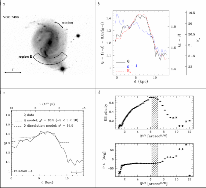
Figure 24: NGC 7496, region E. (c.) Dotted and dashed lines: stellar population models, IMF $M_{\rm upper}=10M_{\sun}$.

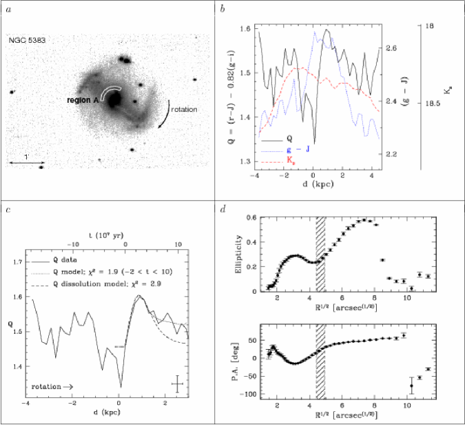
Figure 25: NGC 5383, region A. (c.) Dotted and dashed lines: stellar population models, IMF $M_{\rm upper}=10M_{\sun}$.

Figure 26: NGC 5383, region B. (c.) Dotted and dashed lines: stellar population models, IMF $M_{\rm upper}=10M_{\sun}$.

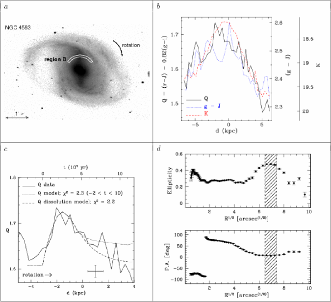
Figure 28: NGC 4593, region B. (c.) Dotted and dashed lines: stellar population models, IMF $M_{\rm upper}=10M_{\sun}$.

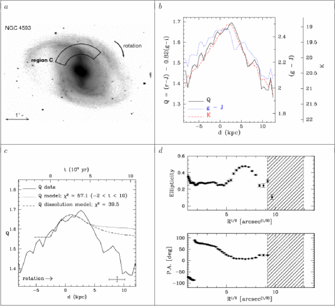
Figure 29: NGC 4593, region C. (c.) Dotted and dashed lines: stellar population models, IMF $M_{\rm upper}=10M_{\sun}$.

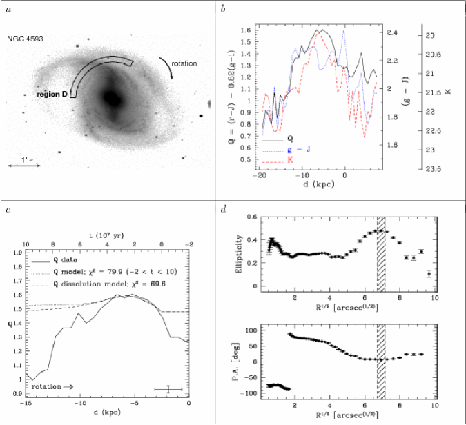
Figure 30: NGC 4593, region D. (c.) Dotted and dashed lines: stellar population models, IMF $M_{\rm upper}=10M_{\sun}$.

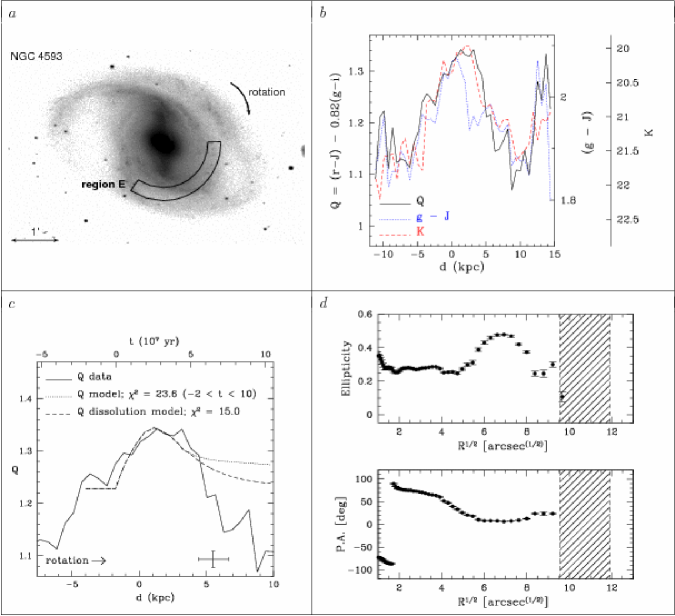
Figure 31: NGC 4593, region E. (c.) Dotted and dashed lines: stellar population models, IMF $M_{\rm upper}=10M_{\sun}$.

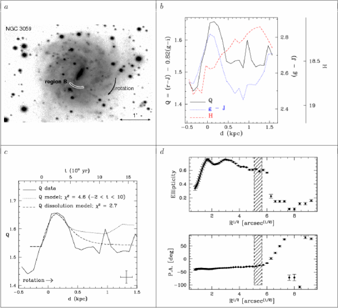
Figure 33: NGC 3059, region B. (d): isophotes from $H$-band mosaic. (c.) Dotted and dashed lines: stellar population models, IMF $M_{\rm upper}=10M_{\sun}$.  

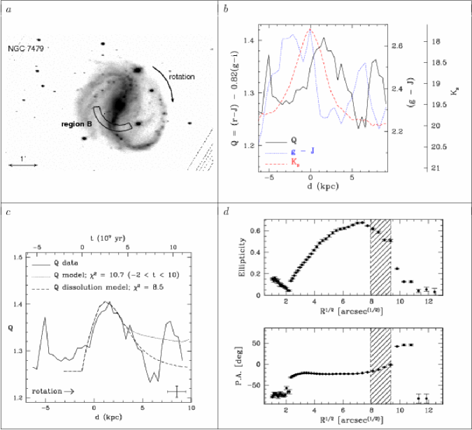
Figure 35: NGC 7479, region B. (c.) Dotted and dashed lines: stellar population models, IMF $M_{\rm upper}=10M_{\sun}$.

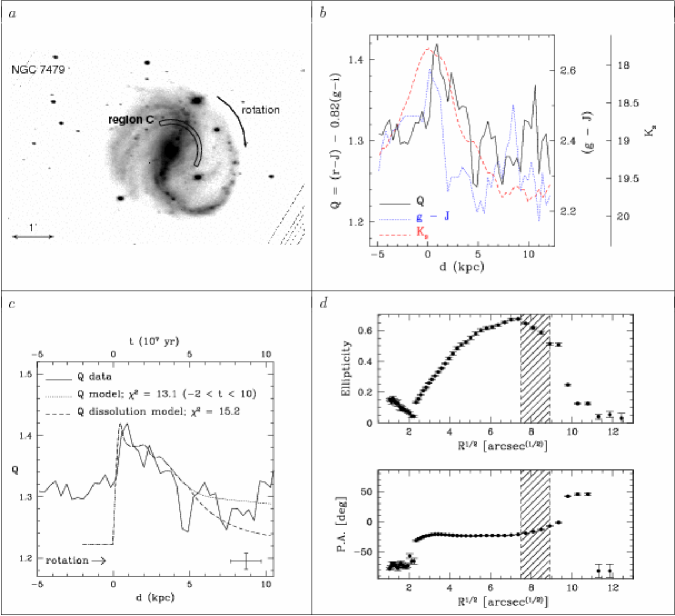
Figure 36: NGC 7479, region C. (c.) Dotted and dashed lines: stellar population models, IMF $M_{\rm upper}=100M_{\sun}$.

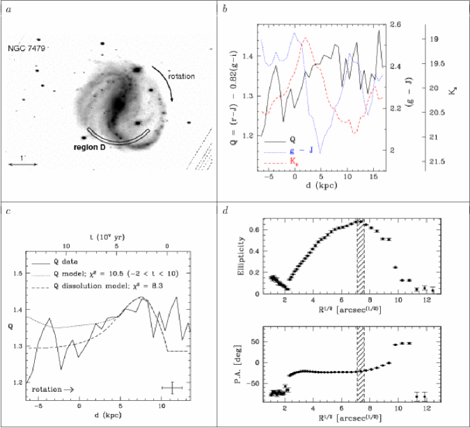
Figure 37: NGC 7479, region D. (c.) Dotted and dashed lines: stellar population models, IMF $M_{\rm upper}=10M_{\sun}$.

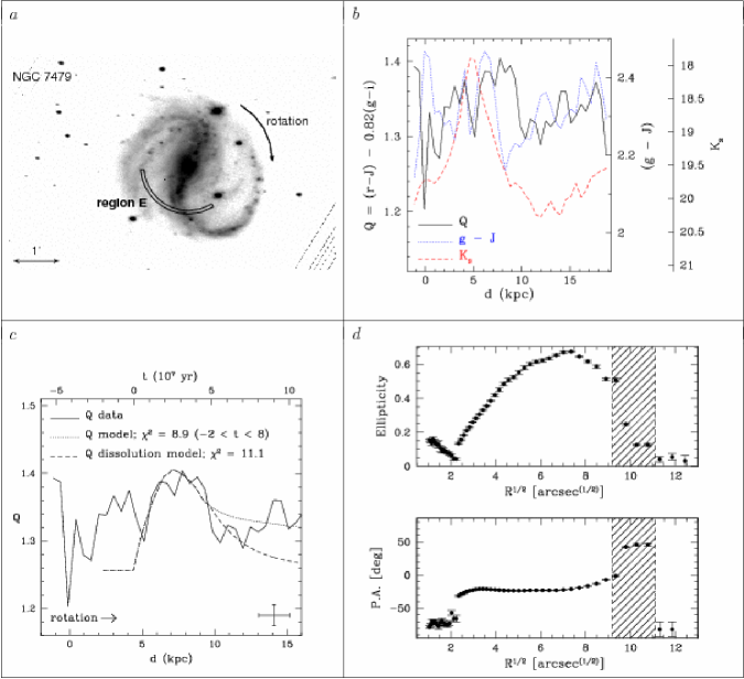
Figure 38: NGC 7479, region E. (c.) Dotted and dashed lines: stellar population models, IMF $M_{\rm upper}=10M_{\sun}$.

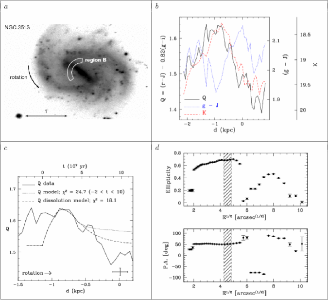
Figure 40: NGC 3513, region B. (d): isophotes from $H$-band mosaic. (c.) Dotted and dashed lines: stellar population models, IMF $M_{\rm upper}=10M_{\sun}$.  

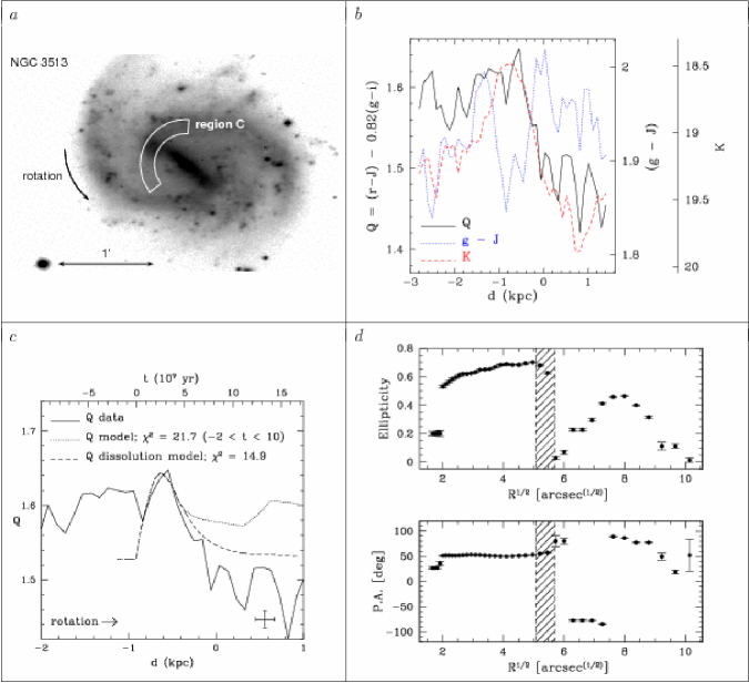
Figure 41: NGC 3513, region C. (d): isophotes from $H$-band mosaic. (c.) Dotted and dashed lines: stellar population models, IMF $M_{\rm upper}=10M_{\sun}$.  

Figure 42: NGC 3513, region D. (d): isophotes from $H$-band mosaic. (c.) Dotted and dashed lines: stellar population models, IMF $M_{\rm upper}=100M_{\sun}$.  

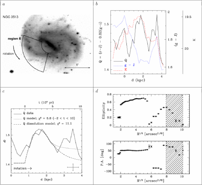
Figure 43: NGC 3513, region E. (d): isophotes from $H$-band mosaic. (c.) Dotted and dashed lines: stellar population models, IMF $M_{\rm upper}=10M_{\sun}$.  

Figure 44: NGC 3513, region F. (d): isophotes from $H$-band mosaic. (c.) Dotted and dashed lines: stellar population models, IMF $M_{\rm upper}=10M_{\sun}$.  

Figure 48: Index $Q(rJgi)$ vs. time for CB07 models, reddened as per the two-component dust model of Charlot & Fall (2000). The duration of the burst is $2\times 10^{7}$ yr, with a Salpeter IMF, $2\%$ by mass of young stars, and solar metallicity. Lower and upper mass limits are 0.1 and 10 $M_{\sun}$, respectively.  

Figure 49: Pattern speed, $\Omega_{\rm p}$, for NGC 7479, obtained from the comparison between observations of color gradient candidates and stellar population synthesis models; the galactocentric radii of the color gradients are indicated in the x-axis. Regions A, B, and C belong to the bar, while regions D and E are located in the spiral arms.

Figure 50: Pattern speed, $\Omega_{\rm p}$, for NGC 3513, obtained from the comparison between observations of color gradient candidates and stellar population synthesis models; the galactocentric radii of the color gradients are indicated in the x-axis. Regions A, B, and C belong to the bar, while regions D, E, and F are located in the spiral arms.

References

- Aguerri et al. (2003) Aguerri, J. A. L., Debattista, V. P., & Corsini, E. M. 2003, MNRAS, 338, 465
- Asif et al. (2005) Asif, M. W., Mundell, C. G., & Pedlar, A. 2005, MNRAS, 359, 408
- Athanassoula (1992) Athanassoula, E. 1992, MNRAS, 259, 345
- Athanassoula (2009) Athanassoula, E. 2009, arXiv:0910.5180
- Athanassoula et al. (2009a) Athanassoula, E., Romero-Gómez, M., & Masdemont, J. J. 2009, MNRAS, 394, 67
- Athanassoula et al. (2009b) Athanassoula, E., Romero-Gómez, M., Bosma, A., & Masdemont, J. J. 2009, MNRAS, 400, 1706
- Athanassoula et al. (2010) Athanassoula, E., Romero-Gómez, M., Bosma, A., & Masdemont, J. J. 2010, MNRAS, 407, 1433
- Barranco & Bernal (2011) Barranco, J., & Bernal, A. 2011, Phys. Rev. D, 83, 043525
- Bastian & Goodwin (2006) Bastian, N., & Goodwin, S. P. 2006, MNRAS, 369, L9
- Benedict et al. (2002) Benedict, G. F., Howell, D. A., Jørgensen, I., Kenney, J. D. P., & Smith, B. J. 2002, AJ, 123, 1411
- Berezinsky et al. (2003) Berezinsky, V. S., Dokuchaev, V. I., & Eroshenko, Y. N. 2003, Phys. Rev. D, 68, 103003
- Berman (2003) Berman, S. L. 2003, A&A, 412, 387
- Bevington & Robinson (2003) Bevington, P. R., & Robinson, D. K. 2003, Data reduction and error analysis for the physical sciences, 3rd ed., by Philip R. Bevington, and Keith D. Robinson. Boston, MA: McGraw-Hill, ISBN 0-07-247227-8, 2003.
- Block et al. (2002) Block, D. L., Bournaud, F., Combes, F., Puerari, I., & Buta, R. 2002, A&A, 394, L35
- Bruzual & Charlot (2003) Bruzual, G., & Charlot, S. 2003, MNRAS, 344, 1000
- Busko (1996) Busko, I. C. 1996, Astronomical Data Analysis Software and Systems V, 101, 139
- Buta & Combes (1996) Buta, R., & Combes, F. 1996, Fundamentals of Cosmic Physics, 17, 95
- Buta & Zhang (2009) Buta, R. J., & Zhang, X. 2009, ApJS, 182, 559
- Buta et al. (2009) Buta, R. J., Knapen, J. H., Elmegreen, B. G., Salo, H., Laurikainen, E., Elmegreen, D. M., Puerari, I., & Block, D. L. 2009, AJ, 137, 4487
- Byrd et al. (1994) Byrd, G., Rautiainen, P., Salo, H., Buta, R., & Crocher, D. A. 1994, AJ, 108, 476
- Carter (1990) Carter, B. S. 1990, MNRAS, 242, 1
- Carter & Meadows (1995) Carter, B. S., & Meadows, V. S. 1995, MNRAS, 276, 734
- Ceverino & Klypin (2007) Ceverino, D., & Klypin, A. 2007, MNRAS, 379, 1155
- Charlot & Fall (2000) Charlot, S., & Fall, S. M. 2000, ApJ, 539, 718
- Combes & Elmegreen (1993) Combes, F., & Elmegreen, B. G. 1993, A&A, 271, 391
- Comerón et al. (2009) Comerón, S., Martínez-Valpuesta, I., Knapen, J. H., & Beckman, J. E. 2009, ApJ, 706, L256
- Contopoulos (1980) Contopoulos, G. 1980, A&A, 81, 198
- Contopoulos & Papayannopoulos (1980) Contopoulos, G., & Papayannopoulos, T. 1980, A&A, 92, 33
- Corsini (2010) Corsini, E. M. 2010, arXiv:1002.1245
- de Vaucouleurs (1963) de Vaucouleurs, G. 1963, ApJS, 8, 31
- de Vaucouleurs et al. (1991) de Vaucouleurs,G., de Vaucouleurs, A., Corwin, H. G., Jr., Buta, R. J., Paturel, G.,& Fouque, P. 1991, Volume 1-3, XII, 2069 pp. 7 figs.. Springer-Verlag Berlin Heidelberg New York (RC3)
- Debattista & Sellwood (2000) Debattista, V. P., & Sellwood, J. A. 2000, ApJ, 543, 704
- Debattista et al. (2002) Debattista, V. P., Corsini, E. M., & Aguerri, J. A. L. 2002, MNRAS, 332, 65
- Dobbs & Pringle (2010) Dobbs, C. L., & Pringle, J. E. 2010, MNRAS, 409, 396
- Dreyer (1888) Dreyer, J. L. E. 1888, MmRAS, 49, 1
- Dubinski et al. (2009) Dubinski, J., Berentzen, I., & Shlosman, I. 2009, ApJ, 697, 293
- Duval & Athanassoula (1983) Duval, M. F., & Athanassoula, E. 1983, A&A, 121, 297
- Efthymiopoulos, C. (2010) Efthymiopoulos, C. 2010, Eur. Phys. J. Special Topics, 186, 91
- Elmegreen & Elmegreen (1985) Elmegreen, B. G., & Elmegreen, D. M. 1985, ApJ, 288, 438
- Elmegreen & Elmegreen (1989) Elmegreen, B. G., & Elmegreen, D. M. 1989, ApJ, 342, 677
- Elmegreen et al. (1992) Elmegreen, B. G., Elmegreen, D. M., Montenegro, L. 1992, ApJS, 79, 37
- Elmegreen (1996) Elmegreen, B. 1996, IAU Colloq. 157: Barred Galaxies, 91, 197
- Elmegreen et al. (2009) Elmegreen, B. G., Galliano, E., & Alloin, D. 2009, ApJ, 703, 1297
- Egusa et al. (2009) Egusa, F., Kohno, K., Sofue, Y., Nakanishi, H., & Komugi, S. 2009, ApJ, 697, 1870
- Erwin & Sparke (1999) Erwin, P., & Sparke, L. S. 1999, ApJ, 521, L37
- Erwin (2004) Erwin, P. 2004, A&A, 415, 941
- Erwin (2009) Erwin, P. 2009, arXiv:0908.0909
- Eskridge et al. (2000) Eskridge, P. B., et al. 2000, AJ, 119, 536
- Eskridge et al. (2002) Eskridge, P. B., et al. 2002, ApJS, 143, 73
- Fathi et al. (2009) Fathi, K., Beckman, J. E., Piñol-Ferrer, N., Hernandez, O., Martínez-Valpuesta, I., & Carignan, C. 2009, ApJ, 704, 1657
- Gabbasov et al. (2009) Gabbasov, R. F., Repetto, P., & Rosado, M. 2009, ApJ, 702, 392
- Gadotti & de Souza (2006) Gadotti, D. A., & de Souza, R. E. 2006, ApJS, 163, 270
- García-Barreto et al. (1996) García-Barreto, J. A., Franco, J., Carrillo, R., Venegas, S., & Escalante-Ramírez, B. 1996, Revista Mexicana de Astronomia y Astrofisica, 32, 89
- Gerssen et al. (1999) Gerssen, J., Kuijken, K., & Merrifield, M. R. 1999, MNRAS, 306, 926
- González et al. (1996) González, R. A., Bruzual A, G., Magris C, G., & Graham, J. R. 1996, New Extragalactic Perspectives in the New South Africa, 209, 243
- González & Graham (1996) González, R. A., & Graham, J. R. 1996, ApJ, 460, 651 (GG96)
- Gieles & Bastian (2008) Gieles, M., & Bastian, N. 2008, A&A, 482, 165
- Gittins & Clarke (2004) Gittins, D. M., & Clarke, C. J. 2004, MNRAS, 349, 909
- Grosbøl et al. (2006) Grosbøl, P., Dottori, H., & Gredel, R. 2006, A&A, 453, L25
- Grosbøl & Dottori (2008) Grosbøl, P., & Dottori, H. 2008, A&A, 490, 87
- Grosbøl & Dottori (2009) Grosbøl, P., & Dottori, H. 2009, A&A, 499, L21
- Grouchy et al. (2010) Grouchy, R. D., Buta, R. J., Salo, H., & Laurikainen, E. 2010, AJ, 139, 2465
- Hamuy et al. (1992) Hamuy, M., Walker, A. R., Suntzeff, N. B., Gigoux, P., Heathcote, S. R., Phillips, M. M. 1992, PASP, 104, 533
- Hamuy et al. (1994) Hamuy, M., Suntzeff, N. B., Heathcote, S. R., Walker, A. R., Gigoux, P., Phillips, M. M. 1994 PASP, 106, 566
- Harsoula et al. (2011) Harsoula, M., Kalapotharakos, C., & Contopoulos, G. 2011, MNRAS, 411, 1111
- Harsoula & Kalapotharakos (2009) Harsoula, M., & Kalapotharakos, C. 2009, MNRAS, 394, 1605
- Hawarden et al. (2001) Hawarden, T. G., Leggett, S. K., Letawsky, M. B., Ballantyne, D. R., Casali, M. M. 2001, MNRAS, 325, 563
- Hohl (1971) Hohl, F. 1971, ApJ, 168, 343
- Isobe et al. (1990) Isobe, T., Feigelson, E. D., Akritas, M. G., & Babu, G. J. 1990, ApJ, 364, 104
- Iye et al. (1982) Iye, M., Okamura, S., Hamabe, M., & Watanabe, M. 1982, ApJ, 256, 103
- Jedrzejewski (1987) Jedrzejewski, R. I. 1987, MNRAS, 226, 747
- Kenney & Lord (1991) Kenney, J. D. P., & Lord, S. D. 1991, ApJ, 381, 118
- Lacey (1984) Lacey, C. G. 1984, MNRAS, 208, 687
- Lacey (1991) Lacey, C. G. 1991, Dynamics of Disc Galaxies, 257
- Laine et al. (2002) Laine, S., Shlosman, I., Knapen, J. H., & Peletier, R. F. 2002, ApJ, 567, 97
- Lamers et al. (2005) Lamers, H. J. G. L. M., Gieles, M., Bastian, N., Baumgardt, H., Kharchenko, N. V., & Portegies Zwart, S. 2005, A&A, 441, 117
- Lynden-Bell (1979) Lynden-Bell, D. 1979, MNRAS, 187, 101
- Martin & Friedli (1997) Martin, P., & Friedli, D. 1997, A&A, 326, 449