Preference elicitation and
inverse reinforcement learning

Abstract

We state the problem of inverse reinforcement learning in terms of preference elicitation, resulting in a principled (Bayesian) statistical formulation. This generalises previous work on Bayesian inverse reinforcement learning and allows us to obtain a posterior distribution on the agent’s preferences, policy and optionally, the obtained reward sequence, from observations. We examine the relation of the resulting approach to other statistical methods for inverse reinforcement learning via analysis and experimental results. We show that preferences can be determined accurately, even if the observed agent’s policy is sub-optimal with respect to its own preferences. In that case, significantly improved policies with respect to the agent’s preferences are obtained, compared to both other methods and to the performance of the demonstrated policy.

1 Introduction

Preference elicitation is a well-known problem in statistical decision theory [10]. The goal is to determine, whether a given decision maker prefers some events to other events, and if so, by how much. The first main assumption is that there exists a partial ordering among events, indicating relative preferences. Then the corresponding problem is to determine which events are preferred to which others. The second main assumption is the expected utility hypothesis. This posits that if we can assign a numerical utility to each event, such that events with larger utilities are preferred, then the decision maker’s preferred choice from a set of possible gambles will be the gamble with the highest expected utility. The corresponding problem is to determine the numerical utilities for a given decision maker.

Preference elicitation is also of relevance to cognitive science and behavioural psychology, e.g. for determining rewards implicit in behaviour [19] where a proper elicitation procedure may allow one to reach more robust experimental conclusions. There are also direct practical applications, such as user modelling for determining customer preferences [3]. Finally, by analysing the apparent preferences of an expert while performing a particular task, we may be able to discover behaviours that match or even surpass the performance of the expert [1] in the very same task.

This paper uses the formal setting of preference elicitation to determine the preferences of an agent acting within a discrete-time stochastic environment. We assume that the agent obtains a sequence of (hidden to us) rewards from the environment and that its preferences have a functional form related to the rewards. We also suppose that the agent is acting nearly optimally (in a manner to be made more rigorous later) with respect to its preferences. Armed with this information, and observations from the agent’s interaction with the environment, we can determine the agent’s preferences and policy in a Bayesian framework. This allows us to generalise previous Bayesian approaches to inverse reinforcement learning.

In order to do so, we define a structured prior on reward functions and policies. We then derive two different Markov chain procedures for preference elicitation. The result of the inference is used to obtain policies that are significantly improved with respect to the true preferences of the observed agent. We show that this can be achieved even with fairly generic sampling approaches.

Numerous other inverse reinforcement learning approaches exist [1, 18, 20, 21]. Our main contribution is to provide a clear Bayesian formulation of inverse reinforcement learning as preference elicitation, with a structured prior on the agent’s utilities and policies. This generalises the approach of Ramachandran and Amir [18] and paves the way to principled procedures for determining distributions on reward functions, policies and reward sequences. Performance-wise, we show that the policies obtained through our methodology easily surpass the agent’s actual policy with respect to its own utility. Furthermore, we obtain policies that are significantly better than those obtained with other inverse reinforcement learning methods that we compare against.

Finally, the relation to experimental design for preference elicitation (see [3] for example) must be pointed out. Although this is a very interesting planning problem, in this paper we do not deal with active preference elicitation. We focus on the sub-problem of estimating preferences given a particular observed behaviour in a given environment and use decision theoretic formalisms to derive efficient procedures for inverse reinforcement learning.

This paper is organised as follows. The next section formalises the preference elicitation setting and relates it to inverse reinforcement learning. Section 3 presents the abstract statistical model used for estimating the agent’s preferences. Section 4 describes a model and inference procedure for joint estimation of the agent’s preferences and its policy. Section 5 discusses related work in more detail. Section 6 presents comparative experiments, which quantitatively examine the quality of the solutions in terms of both preference elicitation and the estimation of improved policies, concluding with a view to further extensions.

2 Formalisation of the problem

We separate the agent’s preferences (which are unknown to us) from the environment’s dynamics (which we consider known). More specifically, the environment is a controlled Markov process $\nu=({\mathcal{S}},{\mathcal{A}},{\mathcal{T}})$, with state space ${\mathcal{S}}$, action space ${\mathcal{A}}$, and transition kernel ${\mathcal{T}}=\left\{\,\tau(\cdot\mid s,a)\mathrel{:}s\in{\mathcal{S}},a\in{\mathcal{A}}\,\right\}$, indexed in ${\mathcal{S}}\times{\mathcal{A}}$ such that $\tau(\cdot\mid s,a)$ is a probability measure on ${\mathcal{S}}$. The dynamics of the environment are Markovian: If at time $t$ the environment is in state $s_{t}\in S$ and the agent performs action $a_{t}\in A$, then the next state $s_{t+1}$ is drawn with a probability independent of previous states and actions:

$$\mathop{\mbox{$\mathbb{P}$}}\nolimits_{\nu}(s_{t+1}\in S\mid s^{t},a^{t})=\tau(S\mid s_{t},a_{t}),\qquad S\subset{\mathcal{S}},$$ (2.1)

where we use the convention $s^{t}\equiv s_{1},\ldots,s_{t}$ and $a^{t}\equiv a_{1},\ldots,a_{t}$ to represent sequences of variables.

In our setting, we have observed the agent acting in the environment and obtain a sequence of actions and a sequence of states:

$$D \mathrel{\triangleq}(a^{T},s^{T}), a^{T} \equiv a_{1},\ldots,a_{T}, s^{T} \equiv s_{1},\ldots,s_{T}.$$

The agent has an unknown utility function, $U_{t}$, according to which it selects actions, which we wish to discover. Here, we assume that $U_{t}$ has a structure corresponding to that of reinforcement learning infinite-horizon discounted reward problems and that the agent tries to maximise the expected utility.

Assumption 1

The agent’s utility at time $t$ is the total $\gamma$-discounted return from time $t$:

$$U_{t}\mathrel{\triangleq}\sum_{k=t}^{\infty}\gamma^{k}r_{k},$$ (2.2)

where $\gamma\in[0,1]$ is a discount factor, and the reward $r_{t}$ is given by the (stochastic) reward function $\rho$ so that $r_{t}\mid s_{t}=s,a_{t}=a\sim\rho(\cdot\mid s,a)$, $(s,a)\in{\mathcal{S}}\times{\mathcal{A}}$.

This choice establishes correspondence with the standard reinforcement learning setting. The controlled Markov process and the utility define a Markov decision process [16] (MDP), denoted by $\mu=({\mathcal{S}},{\mathcal{A}},{\mathcal{T}},\rho,\gamma)$. The agent uses some policy $\pi$ to select actions with distribution $\pi(a_{t}\mid s_{t})$, which together with the Markov decision process $\mu$ defines a Markov chain on the sequence of states, such that:

$$\mathop{\mbox{$\mathbb{P}$}}\nolimits_{\mu,\pi}(s_{t+1}\in S\mid s^{t}) =\int_{\mathcal{A}}\tau(S\mid a,s_{t})\,\mathrm{d}{\pi}(a\mid s_{t}),$$ (2.3)

where we use a subscript to denote that the probability is taken with respect to the process defined jointly by $\mu,\pi$. We shall use this notational convention throughout this paper. Similarly, the expected utility of a policy $\pi$ is denoted by $\mathop{\mbox{$\mathbb{E}$}}\nolimits_{\mu,\pi}U_{t}$. We also introduce the family of $Q$-value functions $\left\{\,Q_{\mu}^{\pi}\mathrel{:}\mu\in{\mathcal{M}},\pi\in{\mathcal{P}}\,\right\}$, where ${\mathcal{M}}$ is a set of MDPs, with $Q_{\mu}^{\pi}:{\mathcal{S}}\times{\mathcal{A}}\to{\mathds{R}}$ such that:

$$Q_{\mu}^{\pi}(s,a)\mathrel{\triangleq}\mathop{\mbox{$\mathbb{E}$}}\nolimits_{\mu,\pi}\left(U_{t}\mid s_{t}=s,a_{t}=a\right).$$ (2.4)

Finally, we use $Q_{\mu}^{*}$ to denote the optimal $Q$-value function for an MDP $\mu$, such that:

$$Q_{\mu}^{*}(s,a)=\sup_{\pi\in{\mathcal{P}}}Q_{\mu}^{\pi}(s,a),\qquad\forall s\in{\mathcal{S}},a\in{\mathcal{A}}.$$ (2.5)

With a slight abuse of notation, we shall use $Q_{\rho}$ when we only need to distinguish between different reward functions $\rho$, as long as the remaining components of $\mu$ remain fixed.

Loosely speaking, our problem is to estimate the reward function $\rho$ and discount factor $\gamma$ that the agent uses, given the observations $s^{T},a^{T}$ and some prior beliefs. As shall be seen in the sequel, this task is easier with additional assumptions on the structural form of the policy $\pi$. We derive two sampling algorithms. The first estimates a joint posterior distribution on the policy and reward function, while the second also estimates a distribution on the sequence of rewards that the agent obtains. We then show how to use those estimates in order to obtain a policy that can perform significantly better than that of the agent’s original policy with respect to the agent’s true preferences.

3 The statistical model

In the simplest version of the problem, we assume that $\gamma,\nu$ are known and we only estimate the reward function, given some prior over reward functions and policies. This assumption can be easily relaxed, via an additional prior on the discount factor $\gamma$ and CMP $\nu$. Let ${\mathcal{R}}$ be a space of reward functions $\rho$ and ${\mathcal{P}}$ to be a space of policies $\pi$. We define a (prior) probability measure $\xi(\cdot\mid\nu)$ on ${\mathcal{R}}$ such that for any $B\subset{\mathcal{R}}$, $\xi(B\mid\nu)$ corresponds to our prior belief that the reward function is in $B$. Finally, for any reward function $\rho\in{\mathcal{R}}$, we define a conditional probability measure $\psi(\cdot\mid\rho,\nu)$ on the space of policies ${\mathcal{P}}$. Let $\rho_{\mathrm{a}},\pi_{\mathrm{a}}$ denote the agent’s true reward function and policy respectively. The joint prior on reward functions and policies is denoted by:

$$\phi(P,R\mid\nu) \mathrel{\triangleq}\int_{R}\psi(P\mid\rho,\nu)\,\mathrm{d}{\xi}(\rho\mid\nu), P \subset{\mathcal{P}},R\subset{\mathcal{R}},$$ (3.1)

such that $\phi(\cdot\mid\nu)$ is a probability measure on ${\mathcal{R}}\times{\mathcal{P}}$.

(a) Basic model

(b) Reward-augmented model

Figure 1: Graphical model, with reward priors $\xi$ and policy priors $\psi$, while $\rho$ and $\pi$ are the reward and policy, where we observe the demonstration $D$. Dark colours denote observed variables and light denote latent variables. The implicit dependencies on $\nu$ are omitted for clarity.

We define two models, depicted in Figure 1. The basic model, shown in Figure 1(a), is defined as follows:

$$\rho \sim\xi(\cdot\mid\nu), \pi\mid\rho_{\mathrm{a}}=\rho \sim\psi(\cdot\mid\rho,\nu),$$

We also introduce a reward-augmented model, where we explicitly model the rewards obtained by the agent, as shown in Figure 1(b):

$$\rho \sim\xi(\cdot\mid\nu), \pi\mid\rho_{\mathrm{a}}=\rho \sim\psi(\cdot\mid\rho,\nu), r_{t}\mid\rho_{\mathrm{a}}=\rho,s_{t}=s,a_{t}=a \sim\rho(\cdot\mid s,a).$$

For the moment we shall leave the exact functional form of the prior on the reward functions and the conditional prior on the policy unspecified. Nevertheless, the structure allows us to state the following:

Lemma 1

For a prior of the form specified in (3.1), and given a controlled Markov process $\nu$ and observed state and action sequences $s^{T},a^{T}$, where the actions are drawn from a reactive policy $\pi$, the posterior measure on reward functions is:

$$\xi(B|s^{T},a^{T},\nu)=\frac{\int_{B}\int_{\mathcal{P}}\pi(a^{T}|s^{T})\,\mathrm{d}{\psi}(\pi|\rho,\nu)\,\mathrm{d}{\xi}(\rho|\nu)}{\int_{\mathcal{R}}\int_{\mathcal{P}}\pi(a^{T}|s^{T})\,\mathrm{d}{\psi}(\pi|\rho,\nu)\,\mathrm{d}{\xi}(\rho|\nu)},$$ (3.2)

where $\pi(a^{T}\mid s^{T})=\prod_{t=1}^{T}\pi(a_{t}|s_{t})$.

Proof.

Conditioning on the observations $s^{T},a^{T}$ via Bayes’ theorem, we obtain the conditional measure:

$$\xi(B\mid s^{T},a^{T},\nu) =\frac{\int_{B}\psi(s^{T},a^{T}\mid\rho,\nu)\,\mathrm{d}{\xi}(\rho\mid\nu)}{\int_{\mathcal{R}}\psi(s^{T},a^{T}\mid\rho,\nu)\,\mathrm{d}{\xi}(\rho\mid\nu)},$$ (3.3)

where $\psi(s^{T},a^{T}\mid\rho,\nu)\mathrel{\triangleq}\int_{\mathcal{P}}\mathop{\mbox{$\mathbb{P}$}}\nolimits_{\nu,\pi}(s^{T},a^{T})\,\mathrm{d}{\psi}(\pi\mid\rho,\nu)$ is a marginal likelihood term. It is easy to see via induction that:

$$\mathop{\mbox{$\mathbb{P}$}}\nolimits_{\nu,\pi}(s^{T},a^{T}) =\prod_{t=1}^{T}\pi(a_{t}\mid s_{t})\tau(s_{t}\mid a_{t-1},s_{t-1}),$$ (3.4)

where $\tau(s_{1}\mid a_{0},s_{0})=\tau(s_{1})$ is the initial state distribution. Thus, the reward function posterior is proportional to:

$$\int_{B}\int_{\mathcal{P}}\prod_{t=1}^{T}\pi(a_{t}|s_{t})\tau(s_{t}|a_{t-1},s_{t-1})\,\mathrm{d}{\psi}(\pi|\rho,\nu)\,\mathrm{d}{\xi}(\rho|\nu).$$

Note that the $\tau(s_{t}|a_{t-1},s_{t-1})$ terms can be taken out of the integral. Since they also appear in the denominator, the state transition terms cancel out. ∎∎

4 Estimation

While it is entirely possible to assume that the agent’s policy is optimal with respect to its utility (as is done for example in [1]), our analysis can be made more interesting by assuming otherwise. One simple idea is to restrict the policy space to stationary soft-max policies:

$$\pi_{\eta}(a_{t}\mid s_{t}) =\frac{\exp(\eta Q_{\mu}^{*}(s_{t},a_{t}))}{\sum_{a}\exp(\eta Q_{\mu}^{*}(s_{t},a))},$$ (4.1)

where we assumed a finite action set for simplicity. Then we can define a prior on policies, given a reward function, by specifying a prior on the inverse temperature $\eta$, such that given the reward function and $\eta$, the policy is uniquely determined.

For the chosen prior (4.1), inference can be performed using standard Markov chain Monte Carlo (MCMC) methods [5]. If we can estimate the reward function well enough, we may be able to obtain policies that surpass the performance of the original policy $\pi_{\mathrm{a}}$ with respect to the agent’s reward function $\rho_{\mathrm{a}}$.

1:for $k=1,\ldots$ do

2:     $\tilde{\rho}\sim\xi(\rho\mid\nu)$.

3:     $\tilde{\eta}\sim\mathop{\mathpzc{Gamma}}\nolimits(\zeta,\theta)$

4:     $\tilde{\pi}=\mathop{\mathpzc{Softmax}}\nolimits(\tilde{\rho},\tilde{\eta},\tau)$

5:     $\tilde{p}=\mathop{\mbox{$\mathbb{P}$}}\nolimits_{\nu,\tilde{\pi}}(s^{T},a^{T})/[\xi(\rho\mid\nu)f_{\mathop{\mathpzc{Gamma}}\nolimits}(\tilde{\eta};\zeta,\theta)]$.

6:     w.p. $\min\left\{\,1,\tilde{p}/p_{(k-1)}\,\right\}$ do

7:         $\pi_{(k)}=\tilde{\pi}$, $\eta_{(k)}=\tilde{\eta}$, $\rho_{(k)}=\tilde{\rho}$, $p_{(k)}=\tilde{p}$.

8:     else

9:         $\pi_{(k)}=\pi_{(k-1)}$, $\eta_{(k)}=\eta_{(k-1)}$, $\rho_{(k)}=\rho_{(k-1)}$, $p_{(k)}=p_{(k-1)}$.

10:     done

11:end for

Algorithm 1 MH: Direct Metropolis-Hastings sampling from the joint distribution $\phi(\pi,\rho\mid a^{T},s^{T})$.

4.1 The basic model: A Metropolis-Hastings procedure

Estimation in the basic model (Fig. 1(a)) can be performed via a Metropolis-Hastings (MH) procedure. Recall that performing MH to sample from some distribution with density $f(x)$ using a proposal distribution with conditional density $g(\tilde{x}\mid x)$, has the form:

$$x_{(k+1)}=\begin{cases}\tilde{x},&\textrm{w.p.~{}}\min\left\{\,1,\frac{f(\tilde{x})/g(\tilde{x}\mid x_{(k)})}{f(x_{(k)})/g(x_{(k)}\mid\tilde{x})}\,\right\}\\ x_{(k)},&\textrm{otherwise}.\end{cases}$$

In our case, $x=(\rho,\pi)$ and $f(x)=\phi(\rho,\pi\mid s^{T},a^{T},\nu)$. We use independent proposals $g(x)=\phi(\rho,\pi|\nu)$. As $\phi(\rho,\pi|s^{T},a^{T},\nu)=\phi(s^{T},a^{T}|\rho,\pi,\nu)\phi(\rho,\pi)/\phi(s^{T},a^{T})$, it follows that:

$$\frac{\phi(\tilde{\rho},\tilde{\pi}\mid s^{T},a^{T},\nu)}{\phi(\rho,\pi\mid s^{T},a^{T},\nu)}=\frac{\mathop{\mbox{$\mathbb{P}$}}\nolimits_{\nu,\tilde{\pi}}(s^{T},a^{T})\phi(\tilde{\rho},\tilde{\pi}\mid\nu)}{\mathop{\mbox{$\mathbb{P}$}}\nolimits_{\nu,\pi_{(k)}}(s^{T},a^{T})\phi(\rho_{(k)},\pi_{(k)}\mid\nu)}.$$

This gives rise to the sampling procedure described in Alg. 1, which uses a gamma prior for the temperature.

4.2 The augmented model: A hybrid Gibbs procedure

The augmented model (Fig. 1(b)) enables an alternative, a two-stage hybrid Gibbs sampler, described in Alg. 2. This conditions alternatively on a reward sequence sample $r_{(k)}^{T}$ and on a reward function sample $\rho_{(k)}$ at the $k$-th iteration of the chain. Thus, we also obtain a posterior distribution on reward sequences.

This sampler is of particular utility when the reward function prior is conjugate to the reward distribution, in which case: (i) The reward sequence sample can be easily obtained and (ii) the reward function prior can be conditioned on the reward sequence with a simple sufficient statistic. While, sampling from the reward function posterior continues to require MH, the resulting hybrid Gibbs sampler remains a valid procedure [5], which may give better results than specifying arbitrary proposals for pure MH sampling.

As previously mentioned, the Gibbs procedure also results in a distribution over the reward sequences observed by the agent. On the one hand, this could be valuable in applications where the reward sequence is the main quantity of interest. On the other hand, this has the disadvantage of making a strong assumption about the distribution from which rewards are drawn.

1:for $k=1,\ldots$ do

2:     $\tilde{\rho}\sim\xi(\rho\mid r^{T}_{(k-1)},\nu)$.

3:     $\tilde{\eta}\sim\mathop{\mathpzc{Gamma}}\nolimits(\zeta,\theta)$

4:     $\tilde{\pi}=\mathop{\mathpzc{Softmax}}\nolimits(\tilde{\rho},\tilde{\epsilon},\tau)$

5:     $\tilde{p}=\mathop{\mbox{$\mathbb{P}$}}\nolimits_{\nu,\tilde{\pi}}(s^{T},a^{T})/[\xi(\rho\mid\nu)f_{\mathop{\mathpzc{Gamma}}\nolimits}(\tilde{\eta};\zeta,\theta)]$.

6:     w.p. $\min\left\{\,1,\tilde{p}/p_{(k-1)}\,\right\}$ do

7:         $\pi_{(k)}=\tilde{\pi}$, $\eta_{(k)}=\tilde{\eta}$, $\rho_{(k)}=\tilde{\rho}$, $p_{(k)}=\tilde{p}$.

8:     else

9:         $\pi_{(k)}=\pi_{(k-1)}$, $\eta_{(k)}=\eta_{(k-1)}$, $\rho_{(k)}=\rho_{(k-1)}$, $p_{(k)}=p_{(k-1)}$.

10:     done

11:     $r^{T}_{(k)}\mid s^{T},a^{T}\sim\rho_{(k)}^{T}(s^{T},a^{T})$

12:end for

Algorithm 2 G-MH: Two stage Gibbs sampler with an MH step

5 Related work

5.1 Preference elicitation in user modelling

Preference elicitation has attracted a lot of attention in the field of user modelling and online advertising, where two main problems exist. The first is how to model the (uncertain) preferences of a large number of users. The second is the problem of optimal experiment design [see 7, ch. 14] to maximise the expected value of information through queries. Some recent models include: Braziunas and Boutilier [4] who introduced modelling of generalised additive utilities; Chu and Ghahramani [6], who proposed a Gaussian process prior over preferences, given a set of instances and pairwise relations, with applications to multiclass classification;  Bonilla et al. [2], who generalised it to multiple users; [13], which proposed an additively decomposable multi-attribute utility model. Experimental design is usually performed by approximating the intractable optimal solution [3, 7].

5.2 Inverse reinforcement learning

As discussed in the introduction, the problems of inverse reinforcement learning and apprenticeship learning involve an agent acting in a dynamic environment. This makes the modelling problem different to that of user modelling where preferences are between static choices. Secondly, the goal is not only to determine the preferences of the agent, but also to find a policy that would be at least as good that of the agent with respect to the agent’s own preferences. Finally, the problem of experiment design does not necessarily arise, as we do not assume to have an influence over the agent’s environment.

5.2.1 Linear programming

One interesting solution proposed by [14] is to use a linear program in order to find a reward function that maximises the gap between the best and second best action. Although elegant, this approach suffers from some drawbacks. (a) A good estimate of the optimal policy must be given. This may be hard in cases where the demonstrating agent does not visit all of the states frequently. (b) In some pathological MDPs, there is no such gap. For example it could be that for any action $a$, there exists some other action $a^{\prime}$ with equal value in every state.

5.2.2 Policy walk

Our framework can be seen as a generalisation of the Bayesian approach considered in [18], which does not employ a structured prior on the rewards and policies. In fact, they implicitly define the joint posterior over rewards and policies as:

$$\phi(\pi,\rho\mid s^{T},a^{T},\nu) =\frac{\exp\left[\eta\sum_{t}Q_{\mu}^{*}(s_{t},a_{t})\right]\xi(\rho\mid\nu)}{\phi(s^{T},a^{T}\mid\nu)},$$

which implies that the exponential term corresponds to $\xi(s^{T},a^{T},\pi\mid\rho)$. This ad hoc choice is probably the weakest point in this approach. Rearranging, we write the denominator as:

$$\xi(s^{T},a^{T}\mid\nu)=\int_{\mathchoice{\hbox to0.0pt{$\displaystyle{{\mathcal{R}}\times{\mathcal{P}}}$\hss}}{\hbox to0.0pt{$\textstyle{{\mathcal{R}}\times{\mathcal{P}}}$\hss}}{\hbox to0.0pt{$\scriptstyle{{\mathcal{R}}\times{\mathcal{P}}}$\hss}}{\hbox to0.0pt{$\scriptscriptstyle{{\mathcal{R}}\times{\mathcal{P}}}$\hss}}}\,\xi(s^{T},a^{T}\mid\pi,\rho,\nu)\,\mathrm{d}{\xi}(\rho,\pi\mid\nu),$$ (5.1)

which is still not computable, but we can employ a Metropolis-Hastings step using $\xi(\rho\mid\nu)$ as a proposal distribution, and an acceptance probability of:

$$\frac{\xi(\pi,\rho\mid s^{T},a^{T})/\xi(\rho)}{\xi(\pi^{\prime},\rho^{\prime}\mid s^{T},a^{T})/\xi(\rho^{\prime})}=\frac{\exp[\eta\sum_{t}Q^{\pi}_{\rho}(s_{t},a_{t})]}{\exp[\eta\sum_{t}Q^{\pi^{\prime}}_{\rho^{\prime}}(s_{t},a_{t})]}.$$

We note that in [18], the authors employ a different sampling procedure than a straightforward MH, called a policy grid walk. In exploratory experiments, where we examined the performance of the authors’ original method [17], we have determined that MH is sufficient and that the most crucial factor for this particular method was its initialisation: as will be also be seen in Sec. 6, we only obtained a small, but consistent, improvement upon the initial reward function.

5.2.3 The maximum entropy approach.

A maximum entropy approach is reported in [22]. Given a feature function $\Phi:{\mathcal{S}}\times{\mathcal{A}}\to{\mathds{R}}^{n}$, and a set of trajectories $\left\{\,s^{T_{k}}_{(k)},a^{T_{k}}_{(k)}\mathrel{:}k=1,\ldots,n\,\right\}$, they obtain features $\Phi^{T_{k}}_{(k)}=\left(\Phi(s_{i,(k)},a_{i,(k)})\right)_{i=1}^{T_{k}}$. They show that given empirical constraints $\mathop{\mbox{$\mathbb{E}$}}\nolimits_{\theta,\nu}\Phi^{T_{k}}=\hat{\mathop{\mbox{$\mathbb{E}$}}\nolimits}\Phi^{T_{k}}$, where $\hat{\mathop{\mbox{$\mathbb{E}$}}\nolimits}\Phi^{T}=\frac{1}{n}\sum_{k=1}^{n}\Phi^{T_{k}}_{(k)}$ is the empirical feature expectation, one can obtain a maximum entropy distribution for actions of the form $\mathop{\mbox{$\mathbb{P}$}}\nolimits_{\theta}(a_{t}\mid s_{t})\propto e^{\theta^{\prime}\Phi(s_{t},a_{t})}$. If $\Phi$ is the identity, then $\theta$ can be seen as a scaled state-action value function.

In general, maximum entropy approaches have good minimax guarantees [12]. Consequently, the estimated policy is guaranteed to be close to the agent’s. However, at best, by bounding the error in the policy, one obtains a two-sided high probability bound on the relative loss. Thus, one is almost certain to perform neither much better, nor much worse that the demonstrator.

5.2.4 Game theoretic approach

An interesting game theoretic approach was suggested by [20] for apprenticeship learning. This also only requires statistics of observed features, similarly to the maximum entropy approach. The main idea is to find the solution to a game matrix with a number of rows equal to the number of possible policies, which, although large, can be solved efficiently by an exponential weighting algorithm. The method is particularly notable for being (as far as we are aware of) the only one with a high-probability upper bound on the loss relative to the demonstrating agent and no corresponding lower bound. Thus, this method may in principle lead to a significant improvement over the demonstrator. Unfortunately, as far as we are aware of, sufficient conditions for this to occur are not known at the moment. In more recent work [21], the authors have also made an interesting link between the error of a classifier trying to imitate the expert’s behaviour and the performance of the imitating policy, when the demonstrator is nearly optimal.

(a) Random MDP

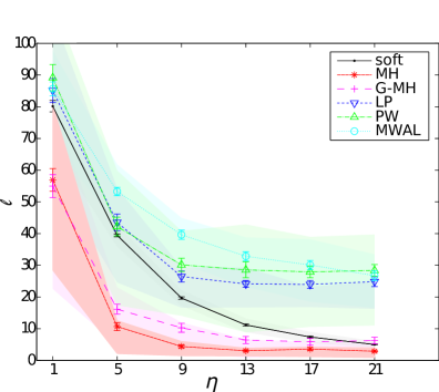
(b) Random Maze

Figure 2: Total loss $\ell$ with respect to the optimal policy, as a function of the inverse temperature $\eta$ of the softmax policy of the demonstrator for (a) the Random MDP and (b) the Random Maze tasks, averaged over 100 runs. The shaded areas indicate the 80% percentile region, while the error bars the standard error.

6 Experiments

6.1 Domains

We compare the proposed algorithms on two different domains, namely on random MDPs and random maze tasks. The Random MDP task is a discrete-state MDP, with four actions, such that each leads to a different, but possibly overlapping, quarter of the state set. The reward function is drawn from a Beta-product hyperprior with parameters $\alpha_{i}$ and $\beta_{i}$, where the index $i$ is over all state-action pairs. This defines a distribution over the parameters $p_{i}$ of the Bernoulli distribution determining the probability of the agent of obtaining a reward when carrying out an action $a$ in a particular state $s$.

For the Random Maze tasks we constructed planar grid mazes of different sizes, with four actions at each state, in which the agent has a probability of $0.7$ to succeed with the current action and is otherwise moved to one of the adjacent states randomly. These mazes are also randomly generated, with the rewards function being drawn from the same prior. The maze structure is sampled by randomly filling a grid with walls through a product-Bernoulli distribution with parameter $1/4$, and then rejecting any mazes with a number of obstacles higher than $|{\mathcal{S}}|/4$.

6.2 Algorithms, priors and parameters

We compared our methodology, using the basic (MH) and the augmented (G-MH) model, to three previous approaches. The linear programming (LP) based approach [14], the game-theoretic approach (MWAL) [20] and finally, the Bayesian inverse reinforcement learning method (PW) suggested in [18]. In all cases, each demonstration was a $T$-long trajectory $s^{T},a^{T}$, provided by a demonstrator employing a softmax policy with respect to the optimal value function.

All algorithms have some parameters that must be selected. Since our methodology employs MCMC the sampling parameters must be chosen so that convergence is ensured. We found that $10^{4}$ samples from the chain were sufficient, for both the MH and hybrid Gibbs (G-MH) sampler, with $2000$ steps used as burn-in, for both tasks. In both cases, we used a gamma prior $\mathop{\mathpzc{Gamma}}\nolimits(1,1)$ for the inverse temperature parameter $\eta$ and a product-beta prior $\mathop{\mathpzc{Beta}}\nolimits^{|S|}(1,1)$ for the reward function. Since the beta is conjugate to the Bernoulli, this is what we used for the reward sequence sampling in the G-MH sampler. Accordingly, the conditioning performed in step $11$ of G-MH is closed-form.

For PW, we used a MH sampler seeded with the solution found by [14], as suggested by [17] and by our own preliminary experiments. Other initialisations, such as sampling from the prior, generally produced worse results. In addition, we did not find any improvement by discretising the sampling space. We also verified that the same number of samples used in our case was also sufficient for this method to converge.

The linear-programming (LP) based inverse reinforcement learning algorithm by Ng and Russell [14] requires the actual agent policy as input. For the random MDP domain, we used the maximum likelihood estimate. For the maze domain, we used a Laplace-smoothed estimate (a product-Dirichlet prior with parameters equal to 1) instead, as this was more stable.

Finally, we examined the MWAL algorithm of Syed and Schapire [20]. This requires the cumulative discounted feature expectation as input, for appropriately defined features. Since we had discrete environments, we used the state occupancy as a feature. The feature expectations can be calculated empirically, but we obtained better performance by first computeing the transition probabilities of the Markov chain induced by the maximum likelihood (or Laplace-smoothed) policy and then calculating the expectation of these features given this chain. We set all accuracy parameters of this algorithm to $10^{-3}$, which was sufficient for a robust behaviour.

6.3 Performance measure

In order to measure performance, we plot the $L_{1}$ loss of the value function of each policy relative to the optimal policy with respect to the agent’s utility:

$$\ell(\pi)\mathrel{\triangleq}\sum_{s\in{\mathcal{S}}}V_{\mu}^{*}(s)-V_{\mu}^{\pi}(s),$$ (6.1)

where $V_{\mu}^{*}(s)\mathrel{\triangleq}\max_{a}Q_{\mu}^{*}(s,a)$ and $V_{\mu}^{\pi}(s)\mathrel{\triangleq}\mathop{\mbox{$\mathbb{E}$}}\nolimits_{\pi}Q_{\mu}^{\pi}(s,a)$.

In all cases, we average over $100$ experiments on an equal number of randomly generated environments $\mu_{1},\mu_{2},\ldots$. For the $i$-th experiment, we generate a $T$-step-long demonstration $D_{i}=(s^{T},a^{T})$ via an agent employing a softmax policy. The same demonstration is used across all methods to reduce variance. In addition to the empirical mean of the loss, we use shaded regions to show $80\%$ percentile across trials and error bars to display the standard error.

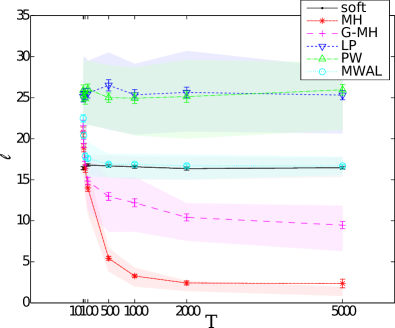
(a) Effect of amount of data

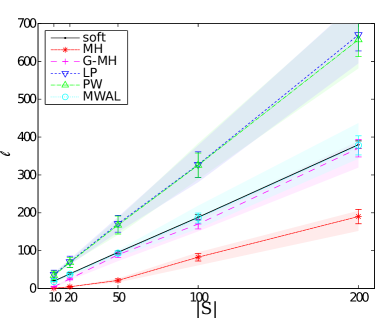
(b) Effect of environment size

Figure 3: Total loss $\ell$ with respect to the optimal policy, in the Random MDP task. Figure 3(a) shows how performance improves as a function of the length $T$. of the demonstrated sequence. Figure 3(b) shows the effect of the number of states $|{\mathcal{S}}|$ of the underlying MDP. All quantities are averaged over 100 runs. The shaded areas indicate the 80% percentile region, while the error bars the standard error.

6.4 Results

We consider the loss of five different policies. The first, soft, is the policy of the demonstrating agent itself. The second, MH, is the Metropolis-Hastings procedure defined in Alg. 1, while G-MH is the hybrid Gibbs procedure from Alg. 2. We also consider the loss of our implementations of Linear Programming (LP), Policy Walk (PW), and MWAL, as summarised in Sec. 5.

We first examined the loss of greedy policies, derived from the estimated reward function, as the demonstrating agent becomes greedier. Figure 2 shows results for the two different domains. It is easy to see that the MH sampler significantly outperforms the demonstrator, even when the latter is near-optimal. While the hybrid Gibbs sampler’s performance lies between that of the demonstrator and the MH sampler, it also estimates a distribution over reward sequences as a side-effect. Thus, it could be of further value where estimation of reward sequences is important. We observed that the performance of the baseline methods is generally inferior, though nevertheless the MWAL algorithm tracks the demonstrator’s performance closely.

This suboptimal performance of the baseline methods in the Random MDP setting cannot be attributed to poor estimation of the demonstrated policy, as can clearly be seen in Figure 3(a), which shows the loss of the greedy policy derived from each method as the amount of data increases. While the proposed samplers improve significantly as observations accumulate, this effect is smaller in the baseline methods we compared against. As a final test, we plot the relative loss in the Random MDP as the number of states increases in Figure 3(b). We can see that the relative performance of methods is invariant to the size of the state space for this problem.

Overall, we observed the basic model (MH) consistently outperforms the agent in all settings. The augmented model (G-MH), while sometimes outperforming the demonstrator, is not as consistent. Presumably, this is due to the joint estimation of the reward sequence. Finally, the other methods under consideration on average do not improve upon the initial policy and can be, in a large number of cases, significantly worse. For the linear programming inverse RL method, perhaps this can be attributed to implicit assumptions about the MDP and the optimality of the given policy. For the policy walk inverse RL method, our belief is that its suboptimal performance is due to the very restrictive prior it uses. Finally, the performance of the game theoretic approach is slightly disappointing. Although it is much more robust than the other two baseline approaches, it never outperforms the demonstrator, even thought technically this is possible. One possible explanation is that since this approach is worst-case by construction, it results in overly conservative policies.

7 Discussion

We introduced a unified framework of preference elicitation and inverse reinforcement learning, presented two statistical inference models, with two corresponding sampling procedures for estimation. Our framework is flexible enough to allow using alternative priors on the form of the policy and of the agent’s preferences, although that would require adjusting the sampling procedures. In experiments, we showed that for a particular choice of policy prior, closely corresponding to previous approaches, our samplers can outperform not only other well-known inverse reinforcement learning algorithms, but the demonstrating agent as well.

The simplest extension, which we have already alluded to, is the estimation of the discount factor, for which we have obtained promising results in preliminary experiments. A slightly harder generalisation occurs when the environment is not known to us. This is not due to difficulties in inference, since in many cases a posterior distribution over ${\mathcal{M}}$ is not hard to maintain (see for example [9, 15]). However, computing the optimal policy given a belief over MDPs is harder [9], even if we limit ourselves to stationary policies [11]. We would also like to consider more types of preference and policy priors. Firstly, the use of spatial priors for the reward function, which would be necessary for large or continuous environments. Secondly, the use of alternative priors on the demonstrator’s policy.

The generality of the framework allows us to formulate different preference elicitation problems than those directly tied to reinforcement learning. For example, it is possible to estimate utilities that are not additive functions of some latent rewards. This does not appear to be easily achievable through the extension of other inverse reinforcement learning algorithms. It would be interesting to examine this in future work.

Another promising direction, which we have already investigated to some degree [8], is to extend the framework to a fully hierarchical model, with a hyperprior on reward functions. This would be particularly useful for modelling a population of agents. Consequently, it would have direct applications on the statistical analysis of behavioural experiments.

Finally, although in this paper we have not considered the problem of experimental design for preference elicitation (i.e. active preference elicitation), we believe is a very interesting direction. In addition, it has many applications, such as online advertising and the automated optimal design of behavioural experiments. It is our opinion that a more effective preference elicitation procedure such as the one presented in this paper is essential for the complex planning task that experimental design is. Consequently, we hope that researchers in that area will find our methods useful.

Acknowledgements

Many thanks to the anonymous reviewers for their comments and suggestions. This work was partially supported by the BMBF Project ”Bernstein Fokus: Neurotechnologie Frankfurt, FKZ 01GQ0840”, the EU-Project IM-CLeVeR, FP7-ICT-IP-231722, and the Marie Curie Project ESDEMUU, Grant Number 237816.

References

- Abbeel and Ng [2004] P. Abbeel and A.Y. Ng. Apprenticeship learning via inverse reinforcement learning. In Proceedings of the 21st international conference on Machine learning (ICML 2004), 2004.
- Bonilla et al. [2010] Edwin V. Bonilla, Shengbo Guo, and Scott Sanner. Gaussian process preference elicitation. In NIPS 2010, 2010.
- Boutilier [2002] C. Boutilier. A POMDP formulation of preference elicitation problems. In AAAI 2002, pages 239–246, 2002.
- Braziunas and Boutilier [2006] Darius Braziunas and Craig Boutilier. Preference elicitation and generalized additive utility. In AAAI 2006, 2006.
- Casella et al. [1999] George Casella, Stephen Fienberg, and Ingram Olkin, editors. Monte Carlo Statistical Methods. Springer Texts in Statistics. Springer, 1999.
- Chu and Ghahramani [2005] W. Chu and Z. Ghahramani. Preference learning with gaussian processes. In Proceedings of the 22nd international conference on Machine learning, pages 137–144. ACM, 2005.
- DeGroot [1970] Morris H. DeGroot. Optimal Statistical Decisions. John Wiley & Sons, 1970.
- Dimitrakakis and Rothkopf [2011] Christos Dimitrakakis and Constantin A. Rothkopf. Bayesian multitask inverse reinforcement learning, 2011. (under review).
- Duff [2002] Michael O’Gordon Duff. Optimal Learning Computational Procedures for Bayes-adaptive Markov Decision Processes. PhD thesis, University of Massachusetts at Amherst, 2002.
- Friedman and Savage [1952] Milton Friedman and Leonard J. Savage. The expected-utility hypothesis and the measurability of utility. The Journal of Political Economy, 60(6):463, 1952.
- Furmston and Barber [2010] Thomas Furmston and David Barber. Variational methods for reinforcement learning. In AISTATS, pages 241–248, 2010.
- Grünwald and Dawid [2004] Peter D. Grünwald and A. Philip Dawid. Game theory, maximum entropy, minimum discrepancy, and robust bayesian decision theory. Annals of Statistics, 32(4):1367–1433, 2004.
- Guo and Sanner [2010] Shengbo Guo and Scott Sanner. Real-time multiattribute bayesian preference elicitation with pairwise comparison queries. In AISTATS 2010, 2010.
- Ng and Russell [2000] Andrew Y. Ng and Stuart Russell. Algorithms for inverse reinforcement learning. In in Proc. 17th International Conf. on Machine Learning, pages 663–670. Morgan Kaufmann, 2000.
- Poupart et al. [2006] P. Poupart, N. Vlassis, J. Hoey, and K. Regan. An analytic solution to discrete Bayesian reinforcement learning. In ICML 2006, pages 697–704. ACM Press New York, NY, USA, 2006.
- Puterman [2005] Marting L. Puterman. Markov Decision Processes : Discrete Stochastic Dynamic Programming. John Wiley & Sons, New Jersey, US, 2005.
- Ramachandran [2010] D Ramachandran, 2010. Personal communication.
- Ramachandran and Amir [2007] D. Ramachandran and E. Amir. Bayesian inverse reinforcement learning. In in 20th Int. Joint Conf. Artificial Intelligence, volume 51, pages 2856–2591, 2007.
- Rothkopf [2008] Constantin A. Rothkopf. Modular models of task based visually guided behavior. PhD thesis, Department of Brain and Cognitive Sciences, Department of Computer Science, University of Rochester, 2008.
- Syed and Schapire [2008] Umar Syed and Robert E. Schapire. A game-theoretic approach to apprenticeship learning. In Advances in Neural Information Processing Systems, volume 10, 2008.
- Syed and Schapire [2010] Umnar Syed and Robert E. Schapire. A reduction from apprenticeship learning to classification. In NIPS 2010, 2010.
- Ziebart et al. [2010] Brian D. Ziebart, J. Andrew Bagnell, and Anind K. Dey. Modelling interaction via the principle of maximum causal entropy. In Proceedings of the 27th International Conference on Machine Learning (ICML 2010), Haifa, Israel, 2010.