Molecular Dynamics Simulation Study of Nonconcatenated Ring Polymers in a Melt: I. Statics

Abstract

Molecular dynamics simulations were conducted to investigate the structural properties of melts of nonconcatenated ring polymers and compared to melts of linear polymers. The longest rings were composed of $N=1600$ monomers per chain which corresponds to roughly 57 entanglement lengths for comparable linear polymers. For the rings, the radius of gyration squared, $\langle R_{g}^{2}\rangle$, was found to scale as $N^{4/5}$ for an intermediate regime and $N^{2/3}$ for the larger rings indicating an overall conformation of a crumpled globule. However, almost all beads of the rings are “surface beads” interacting with beads of other rings, a result also in agreement with a primitive path analysis performed in the next paperHalverson et al. (2011). Details of the internal conformational properties of the ring and linear polymers as well as their packing are analyzed and compared to current theoretical models. [DOI: 10.1063/1.3587137]

I Introduction

Understanding the static and dynamic properties of ring polymer melts is one of the remaining challenges in polymer science. Unlike linear polymers, the topological constraints for ring or cyclic polymers are permanent and this affects both their static and dynamic properties. For linear polymers the topological constraints imposed by the non-crossability of the chains (entanglements) force each chain to diffuse along its own coarse-grained backbone, the so-called primitive path, and this is well described by the reptation model of de Gennes and Edwards. For branched systems strands have to fold back in order to find a new conformation without crossing any other chain, resulting in an exponential growth of the longest relaxation time due to the entropy barrier of ${\cal O}(\mathrm{strand~{}length})$ between different statesde Gennes (1971, 1979); Doi and Edwards (1986). A number of simulations and experimental results confirm this conceptTobolsky (1960); Onogi et al. (1970); Berry and Fox (1968); Casale et al. (1971); Odani et al. (1972); Kremer and Grest (1990); Binder (1995); McLeish (2002); Everaers et al. (2004). For both linear and branched polymer melts, it is the free chain ends that make the known relaxation mechanisms possible. However, in the case of rings there are no free ends. This raises a number of unanswered questions regarding the motion and stress relaxation of ring polymer melts based on their different conformational properties, which will be discussed in the subsequent paperHalverson et al. (2011).

Understanding a melt of nonconcatenated and unknotted rings is also closely related to the problem of the compact globular state of an unknotted loop. Grosberg et al. Grosberg et al. (1988) were the first to hypothesize that the equilibrium state of a compact unknotted loop is the so-called crumpled globule, in which each subchain is condensed in itself, and, therefore, the polymer backbone is self-similar with a fractal dimension of 3. The idea behind this prediction is that two pieces of the chain, each of them crumpled, act pretty much like two nonconcatenated rings, and the latter system obviously experiences at least some volume exclusion for topological reasons (on this subject see recent work Bohn et al. (2010) and references therein). A direct test of this prediction was first made by Lua et al. Lua et al. (2004) by modeling the closed Hamiltonian loops on the compact domains of a cubic lattice. Some evidence of segregation between globules on the chain was observed, but overall the results were inconclusive because the simulated chains were too short or the statistics were too poor.

Squeezing topologically constrained rings against each other in a melt, or squeezing one unknotted ring against itself in a restricted volume, is also a problem of great potential significance in application to the DNA organization in the cell nucleus. Chromatin fibers are packed in vivo at a rather high density, with volume fractions not dissimilar to those in a polymer melt. However, unlike a melt of linear chains, the different chromosomes in the nucleus do not intermix, but stably occupy different distinct “territories”: the image in which each chromosome is stained with a different color resembles a political map of some continent Cremer and Cremer (2001) (see also reviews Cremer et al. (2006); Meaburn and Misteli (2007)). This makes an obvious analogy with the melt of nonconcatenated rings; indeed, if the rings in the simulated melt are shown in different colors, the image of a political map emergesVettorel et al. (2009). This strongly suggests topological properties of chromatin chains as a likely mechanism behind chromosome segregation, similar to segregation of nonconcatenated rings in the meltVettorel et al. (2009); Blackstone et al. (2011); Dorier and Stasiak (2009). Why the topology of the chromatin fibers is restricted is a somewhat open question, but it might be that the DNA ends are attached to the nuclear envelope, or simply that the cell lifetime is not long enough for reptation to develop Sikorav and Jannink (1994); Rosa and Everaers (2008); Vettorel and Kremer (2010). Territorial segregation of chromosomes appears to be a common feature for the cells of higher eukaryotes, including humans, but it is less well pronounced or absent altogether in lower eukaryotes such as yeast Meaburn and Misteli (2007); Duan et al. (2010); Therizols et al. (2010). This observation is at least qualitatively consistent with the fact that topological segregation of nonconcatenated loops is fully developed only when polymers are very long.

In recent years, more detailed information on chromatin fiber organization has become available, due to the advent of novel experimental techniques, such as Fluorescence In Situ Hybridization FISH Solovei et al. (2002) and HiC, which is a generalization of 3C (Comprehensive Chromosome Capture)Dekker et al. (2003) and 4C (the same on a Chip)Simonis et al. (2006). These methods allow one to probe the large scale features of the chromatin fiber fold in a single chromosome. In particular, the HiC study of human genome folding Lieberman-Aiden et al. (2009) revealed the signature of a fractal folding pattern which was explicitly associated with the crumpled globule organization of DNA originally predicted on purely theoretical grounds Grosberg et al. (1993). Specifically, the measurement indicated that the loop factor $P(s)$ (the probability that two loci of genetic distance $s$ base-pairs apart will be found spatially next to each other in chromosome) scales as $P(s)\sim s^{-\gamma}$ over the interval of $s$, roughly, $0.5\ \mathrm{Mbp}\lesssim s\lesssim 7\ \mathrm{Mbp}$, where the power $\gamma$ is 1 or slightly higher. This scaling appears to be consistent with the crumpled globule model Rosa et al. (2010). There are also many more indications of self-similarity, or scale-invariance, in the chromatin folding (see recent review Bancaud et al. (2010) and references therein). Current biological theories about these issues also actively involve dynamical aspects, how this presumably crumpled self-similar structure can move to perform its functions. To this end, there are some observations regarding the structural difference between the active part of the chromatin fiber, currently transcribed, and the more densely packed, non-transcribing heterochromatin Lieberman-Aiden et al. (2009). Without going into further detail, suffice it to say for the purposes of the present paper that chromosome studies necessitate the further and deeper understanding of the melt of nonconcatenated rings, both in equilibrium and in dynamics, as a basic elementary model.

Recent theories for melts of nonconcatenated rings or the globule of a single unknotted ring have been dominated by the idea that the topological constraints imposed on a given ring by the surrounding ones, as well as the constraints imposed by the different parts of the same ring on each other, can be treated using a sort of a “topological mean field”, namely, by considering a single ring immersed in a lattice of immobile topological obstacles Cates, M.E. and Deutsch, J.M. (1986); Khokhlov and Nechaev (1985); Rubinstein (1986); Nechaev et al. (1987); Obukhov et al. (1994), with none of the obstacles piercing through the ring (such that the ring is nonconcatenated with the whole lattice). The conformation of a ring in such a lattice represents a lattice animal with every bond traversed by the polymer twice (in opposite directions). We emphasize that the structure of branches in the lattice animal is completely annealed. In the off-lattice case, a similar annealed randomly-branched structure is expected, in which the chain follows itself twice along every branch only down to a certain scale $d$, similar to the distance between obstacles or the tube diameter in reptation theory. Such structure is reasonable as long as $l_{k}\ll d\ll\left\langle R_{g}\right\rangle$, where $l_{k}$ is the Kuhn length and $\left\langle R_{g}\right\rangle$ is the average gyration radius of the loop. Based on the lattice animal model, Cates and Deutsch Cates, M.E. and Deutsch, J.M. (1986) modified Flory’s argument and arrived at the conjecture that $\left\langle R_{g}(N)\right\rangle\sim N^{2/5}$ for the nonconcatenated unknotted rings in the melt. An alternative theory, also based on the lattice-of-obstacles picture, but consistent with the crumpled globule model for a single ring chain Grosberg et al. (1988), suggested that rings in the melt are compact objects in the sense that $\left\langle R_{g}(N)\right\rangle\sim N^{1/3}$. Lacking any systematic theoretical approaches and based on purely heuristic arguments, this controversy has remained unresolved.

Experimental efforts to synthesize melts of pure rings have suffered from difficulties in purification and polydispersity. Early studies considered polystyrene and polybutadiene ring polymers synthesized in both good and theta solvent conditions.Hild et al. (1983); Roovers and Toporowski (1983); McKenna et al. (1987); Roovers and Toporowski (1988) However, due to the presence of linear chain contaminants and the possible presence of knotted conformations, these works have been received with skepticism. More recently ring polymers were isolated from linear chains having roughly the same molecular weight with a very high degree of separation.Pasch and Trathnigg (1997); Lee et al. (2000) The concentration of linear chains is estimated to be less than one chain in a thousand. For these systems, however, only dynamical properties have been reported. Kapnistos et al. have made stress relaxation measurements for these samples as well as samples that were contaminated systematically with linear chains.Kapnistos et al. (2008) The authors claim that the viscoelastic response of the system was significantly affected already at concentrations of linear contaminants well below the overlap concentration. The effect of linear contaminants will be investigated in a separate paperHalverson et al. . Nam et al. have synthesized and investigated melts of low-molecular-weight polydimethylsiloxane ringsNam et al. (2009). Synthesizing and isolating pure, monodisperse, unknotted and nonconcatenated rings remains a major challenge and thus computer simulations of perfectly controlled systems can be very helpful to learn more about these melts.

The early theoretical investigations were followed by a series of computational studies. Müller et al. (1996); Brown and Szamel (1998); Müller et al. (2000); Brown and Szamel (1998); Müller et al. (2000); Brown et al. (2001); Suzuki et al. (2008); Vettorel et al. (2009, 2009); Suzuki et al. (2009) In the first work Müller et al. (1996), the bond fluctuation model (BFM) Carmesin and Kremer (1988) was employed, and rings up to $N=512$ monomers were examined at the density of $0.5$ (in units of occupied lattice sites). The first results appeared to support the Cates and Deutsch conjectureCates, M.E. and Deutsch, J.M. (1986), that $\left\langle R_{g}\right\rangle\sim N^{2/5}$. However, the entanglement length for linear BFM chains at a density of $0.5$ is known to be fairly large, $N_{e,\mathrm{linear}}>70$. Therefore, the rings examined in this work are still fairly short, less than $7N_{e,\mathrm{linear}}$, they cannot be expected to be “asymptotic”. In the second study from the same groupMüller et al. (2000) the chain length was extended to $N=1024$ and also stiffer chains were considered, which at the same density have a smaller entanglement length. Although a crossover to $\left\langle R_{g}\right\rangle\sim N^{1/3}$ was observed, the ultimate scaling could not be settled because the overall structure of the stiff ring polymers did not resemble a collapsed globule, being quite extended to accommodate the higher bending energies. More recently some of us studied a melt of nonconcatenated flexible rings on a simple cubic lattice for chain lengths up to $N=10000$Vettorel et al. (2009). This was achieved by a special Monte Carlo method which included nonlocal moves to speed-up the relaxationVettorel et al. (2009). While the simulations were started from qualitatively different initial conformations (collapsed globules, extended double stranded paths and growing chains) the equilibrium properties were found to be the same. For large rings, Vettorel et al. Vettorel et al. (2009) found the $\left\langle R_{g}^{2}\right\rangle^{1/2}\sim N^{1/3}$ scaling with a wide crossover which can be interpreted as a $2/5$ intermediate “asymptotics”. Suzuki et al.Suzuki et al. (2009) have also reproduced the $1/3$ scaling regime. All these works have left not only several static properties but essentially all dynamic properties unexplored.

In the first of two papers, we investigate the static properties of ring polymer melts using molecular dynamics (MD) simulation. To our knowledge the only previous MD studies of ring polymer melts are by Hur et al. Hur et al. (2006) and Tsolou et al. Tsolou et al. (2010) who considered polyethylene for short chain lengths (i.e., $N\lesssim 3N_{e,\mathrm{linear}}$), and Hur et al. Hur et al. (2011) for chain lengths up to about $11N_{e,\mathrm{linear}}$, where $N_{e,\mathrm{linear}}$ is the entanglement molecular weight of the linear polymer system. Here we consider ring and linear melts composed of much longer chains. The number of monomers per ring ranges from 100 to 1600 or $3N_{e,\mathrm{linear}}$ to $57N_{e,\mathrm{linear}}$ The linear chain melts were simulated using the same model as the rings with chain lengths varying from 100 to 800 monomers per chain. Such highly entangled melts have very long relaxation times and a highly parallelized simulation code was used. For the longest rings as many as 2048 IBM Blue Gene/P cores were used for a single simulation.

The simulation model is presented in Section II.1. This is followed by a description of the melt preparation and the simulation protocol in Section II.2. The static properties for the ring and linear melts are reported in Section III followed by a comprehensive discussion of the results in Section IV, while the key findings of the work and future challenges are presented in the Conclusions section. Dynamic properties based on the same simulation runs are presented in the subsequent paperHalverson et al. (2011).

II Simulation Methodology

II.1 Model

Based on the Kremer-Grest (KG) model Kremer and Grest (1990), all beads interact via a shifted Lennard-Jones potential (WCA or Weeks-Chandler-Anderson potential) (Eq. 1) with a cutoff of $r_{c}=2^{1/6}~{}\sigma$. Covalently bonded monomers between nearest neighbor beads along the chain also interact via the finitely extensible nonlinear elastic (FENE) potential (Eq. 2). Chain stiffness is introduced by an angular potential (Eq. 3), where $\theta_{i}$ is the angle between bonds connecting beads $i-1$, $i$ and $i$, $i+1$.Everaers et al. (2004) For all ring and linear polymer simulations reported in this work: $k=30~{}\epsilon/\sigma^{2}$, $R_{0}=1.5~{}\sigma$ and $k_{\theta}=1.5~{}\epsilon$.

$$\frac{U(r_{ij})}{4\epsilon}=\begin{cases}\left[\left(\frac{\sigma}{r_{ij}}\right)^{12}-\left(\frac{\sigma}{r_{ij}}\right)^{6}\right]+\frac{1}{4},&r_{ij}\leq 2^{1/6}~{}\sigma\\ 0,&r_{ij}>2^{1/6}~{}\sigma\end{cases}$$ (1)

$$U(r_{ij})=\begin{cases}-0.5kR_{0}^{2}\ln[1-(r_{ij}/R_{0})^{2}],&r_{ij}<R_{0}\\ \infty,&r_{ij}\geq R_{0}\end{cases}$$ (2)

$$U_{\mathrm{angle}}(\theta_{i})=k_{\theta}[1-\cos(\theta_{i}-\pi)].$$ (3)

The natural time scale of Eq. 1 is $\tau=\sigma\sqrt{m/\epsilon}$, where $m$ is the mass of a monomer. For the simulations we use $T=1.0~{}\epsilon/k_{B}$ and $\rho=0.85~{}\sigma^{-3}$. This model has been frequently used for simulation studies of polymer melts and solutions, so that one can refer to ample information throughout the discussion of the present, new results. The linear chain data presented in this work is all new as well. The ring melts were simulated using 200 polymers of length 100 to 1600 monomers per chain. The linear systems were composed of $2500$ chains of length $N=100$, 250 chains of $N=200$, and 400 chains of length $N=400$ and 800 (cf. Table 1). An important parameter for our discussion is the entanglement length for linear polymers in a melt. For the model employed here this parameter was determined Everaers et al. (2004) to be

$$N_{e,\mathrm{linear}}=28\pm 1\ .$$ (4)

Comparing $N_{e,\mathrm{linear}}$ for different simulation models and different chemical species allows one to compare equivalent chain lengths from rather different studies.

	Rings			Linear
$N$	$M$	$L/\sigma$	$\tau_{R}/10^{5}~{}\tau$	$M$	$L/\sigma$	$\tau_{R}/10^{5}~{}\tau$
100	200	28.655	0.10	2500	66.503	0.38
200	200	36.103	0.39	250	38.891	1.57
400	200	45.487	1.59	400	57.287	6.36
800	200	57.310	6.29	800	72.176	25.2
1600	200	72.207	25.2	–	–	–

Table 1: System parameters for the ring and linear melt simulations. All simulations were performed with $k_{B}T=\epsilon$ and $\rho\sigma^{3}=0.85$ in a cubic box of side $L$. The number of monomers per chain is $N$ and the number of chains is $M$. The Rouse times Doi and Edwards (1986); Tsolou et al. (2010) are $\tau_{R,\mathrm{linear}}=N\langle R_{e,\mathrm{linear}}^{2}\rangle\zeta/3\pi^{2}k_{B}T$ and $\tau_{R,\mathrm{rings}}=\tau_{R,\mathrm{linear}}/4$. The friction coefficient, $\zeta$, was estimated from the initial mean-square displacement dataPütz et al. (2000) of the inner monomers of the $N=100$ linear system to be $43~{}\tau^{-1}$. It is found to be 25% lower if the initial ring data are used.

II.2 Preparation and Production Runs

The linear chain melts were prepared following the procedure outlined in Auhl et al.Auhl et al. (2003) Initially the chains are grown as random walks and placed randomly in the simulation cell without regard to monomers overlapping. The overlaps are removed using a soft potential whose strength is increased slowly over a few hundred thousand time steps. The Lennard-Jones potential is then turned on. The system is further equilibrated using the double-bridging algorithm in which new bonds are formed across a pair of chains, creating two new chains each substantially different from the original. This combination of methods has proven to be a very efficient approach to equilibrate long chain melts.Auhl et al. (2003)

For ring melts the situation is more complex, as we do not have well known target conformations. However, from the earlier lattice studies we have some insight about the general conformations Vettorel et al. (2009). The initial configuration for each ring melt simulation was prepared via the following steps Vettorel and Kremer (2010). Rings were constructed with their centers at the sites of a simple cubic lattice. The monomers of each chain were created on a circular path in a plane with a random orientation. By choosing the lattice constant to be larger than the ring diameter this procedure ensures that the rings are unknotted and nonconcatenated. An intrachain attractive interaction was then used to collapse the rings. This was done by increasing the cutoff distance in Eq. 1 to $r_{c}=2.5~{}\sigma$. The interchain interactions remain purely repulsive during this phase. For the $N=1600$ system, an additional force proportional to the distance between a monomer and the center-of-mass of the chain, was added in order to speed-up the initial contraction.

The density of the system was initially low because the rings were widely spaced. A short NPT simulation for $500~{}\tau$ was carried out to increase the density of the system to the target value ($\rho=0.85~{}\sigma^{-3}$). During this phase the applied pressure was slowly increased and the intrachain attraction was kept on. Once the target density had been reached the NPT ensemble was switched to the NVT ensemble. The attractive part of the intrachain bead-bead interaction was switched off and the simulations were continued up to about three times the Rouse time of each system. The Rouse times for the ring systems are given in Table 1. During this equilibration phase the rings diffused a distance of at least their own diameter. Taking the typical radius of gyration, in units of the entanglement length, the conformations then compare well to our previous lattice Monte Carlo results on very long ring polymersVettorel et al. (2009). In the course of the following very long simulations, we also carefully monitored possible changes in the instantaneous averages of the spanning diameters and radii of gyration of the rings in order to observe any drift pointing towards poor equilibration. Within the accuracy of our data, we did not observe any drift anymore in all data used for analysis. This is especially important for ring polymers starting with somewhat artificial initial configurationsVettorel et al. (2009).

The production runs were carried out in the NVE ensemble with a weak coupling to a Langevin thermostat Schneider and Stoll (1978); Kremer and Grest (1990) to maintain the temperature. A cubic simulation box with periodic boundary conditions in all dimensions was used for each simulation. The velocity Verlet method was used to numerically integrate Newton’s equations of motion. The ring simulations were performed using ESPResSo Limbach et al. (2006) and LAMMPS Plimpton (1995) with a time step and friction coefficient of 0.01 $\tau$ and $1.0~{}\tau^{-1}$, respectively. LAMMPSPlimpton (1995) was used for the linear systems with a time step of 0.012 $\tau$ and a friction coefficient of $0.5~{}\tau^{-1}$. In computing mean-square displacements the center-of-mass drift of the system was removed. Table 1 gives the system parameters for the ring and linear simulations.

III Conformational and Structural Properties

The equilibration of $R_{g}^{2}$ is shown for the ring systems in Fig. 1. The larger chains are found to increase in size before fluctuating about an average value while $R_{g}^{2}(t)$ for the smaller chains changes very little over the course of the simulation compared to the initial starting conformations. Although long simulation times are needed to equilibrate the systems, particularly with large $N$, our runs are long enough because as shown in Fig. 1, even for the $N=1600$ case, the time window over which average quantities were computed is about ten times longer than the time required for the system to reach equilibrium. All quantities reported in the present and subsequent paper are exclusively based on the simulation regime where the polymers are fully equilibrated. The time window of this regime is approximately five times the longest correlation time of the $N=1600$ ring system, as determined by various quantities (cf. subsequent paper on dynamicsHalverson et al. (2011)). The linear systems have longer relaxation times and the simulation time of the $N=800$ linear system did not exceed the longest relaxation time (see below).

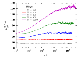
Figure 1: Radius of gyration squared as a function of time for the five ring systems.

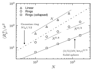
Figure 2: Equilibrium values of the radius of gyration squared $\left\langle R_{g}^{2}\right\rangle$ versus $N$ for the ring and linear systems. The dashed lines indicate the crossover and asymptotic scaling regimes of the rings. The collapsed ring data was found by simulating single rings in vacuum with $r_{c}=2.5~{}\sigma$. The solid line corresponds to a homogeneous sphere or $\left\langle R_{g}^{2}\right\rangle=(3/5)(3N/4\pi\rho)^{2/3}$ with $\rho\sigma^{3}=0.85$. The error bars for all data points are smaller than the symbol sizes.

Fig. 2 shows the equilibrium average values of $R_{g}^{2}$ versus $N$ for the ring and linear systems. The linear chains in the melt exhibit the expected Gaussian behavior or $\left\langle R_{g}^{2}\right\rangle\sim N$. We have to emphasize that this Gaussian behavior is not altered by the recently discovered slowly decaying tangent-tangent correlation along the chain in the melt Wittmer et al. (2004, 2007). As Fig. 3 demonstrates, the tangent-tangent correlation between two points on the chain in the melt decays as $s^{-3/2}$ with contour distance $s$, unlike exponential decay for the ideal chain in a dilute solution. In our system, unlike the simulations of Wittmer et al. Wittmer et al. (2004, 2007), we also observe an initial exponential decay of the correlation at small $s$ because our chains have some significant bending rigidity (see above). The algebraic decay of the tangent-tangent correlation does not alter the conclusion that linear chains in the melt are Gaussian in the sense of a normal distribution of the end-to-end distances or simply the linear scaling of $\left\langle R_{g}^{2}\right\rangle$ with $N$. This is simply because the sum of $s^{-3/2}$ converges at large $s$, indicating that an effective segment comprises only a finite number of monomers.

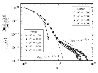
Figure 3: Tangent-tangent correlation function against contour distance between points, $s$, in double logarithmic scale. The correlation function is found to decay much more rapidly for the rings (solid line) than the linear chains (dotted line).

The ring systems show various regimes depending on their lengths. For small $N$ they appear Gaussian. An extended crossover regime then follows where $\left\langle R_{g}^{2}\right\rangle\sim N^{4/5}$. Finally, the longest chains approach a $N^{2/3}$ scaling, showing that very long ring polymers, with $N\gtrsim 400\approx 15N_{e,\mathrm{linear}}$ (see Eq. (4)) are required to approach the asymptotic regime. Exactly the same is observed for the spanning distance squared $R_{e}^{2}(N)$ of the rings, which is defined as the mean-square distance between monomers $1$ and $N/2+1$ (or $k$ and $k+N/2$ with any $k$) in the ring (cf. Table 2). These results are in agreement with previous simulations Vettorel et al. (2009).

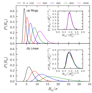
Figure 4: Probability distribution function of the radius of gyration for the (a) rings and (b) linear chains. The insets show the probability distribution function of $R_{g}$ normalized by its root-mean-square value.

The equilibrium fluctuations of the gyration radius are given in Fig. 4 for each of the ring and linear systems. In this paragraph we reserve the notation $R_{g}$ for the instantaneous (fluctuating) value of the gyration radius, while the mean-square gyration radius is written as $\left\langle R_{g}^{2}\right\rangle$. The distributions become wider and asymmetrical with increasing $N$, however they follow a perfect scaling when normalized by $\left\langle R_{g}^{2}\right\rangle^{1/2}$. The insets to Fig. 4 give the probability distribution functions of $R_{g}$ normalized by the respective root-mean-square values for the (a) rings and (b) linear chains. All five data sets for rings of different lengths are found to collapse nearly perfectly onto a single curve. For the linear chains, while data for $N=100$, $200$, and $400$ collapse about as well as for the rings, the distribution for the $N=800$ case slightly deviates from the others. This is indicative of a system that may not have been completely equilibrated despite an extremely long simulation time. Some properties are more sensitive to improper equilibration than others. For this work only the shear relaxation modulus, which is discussed in the subsequent paper, is affected by the lack of equilibration for the $N=800$ linear case. Our data suggest that all other linear and ring systems are properly equilibrated.

	Rings				Linear
$N$	$\left\langle R_{g}^{2}\right\rangle/\sigma^{2}$	$\left\langle R_{e}^{2}\right\rangle/\sigma^{2}$	$\langle\lambda_{1}\rangle/\langle\lambda_{3}\rangle$	$\langle\lambda_{2}\rangle/\langle\lambda_{3}\rangle$	$\left\langle R_{g}^{2}\right\rangle/\sigma^{2}$	$\left\langle R_{e}^{2}\right\rangle/\sigma^{2}$	$\langle\lambda_{1}\rangle/\langle\lambda_{3}\rangle$	$\langle\lambda_{2}\rangle/\langle\lambda_{3}\rangle$
100	17.2 (0.4)	50.8 (1.5)	6.4	2.3	43.4 (1.2)	263.8 (1.6)	12.9	2.8
200	30.8 (0.7)	88.8 (2.7)	5.9	2.2	88.9 (1.2)	538.9 (1.6)	12.6	2.8
400	52.9 (1.2)	149.4 (4.8)	5.5	2.1	180.8 (1.3)	1095.3 (1.6)	12.3	2.8
800	87.6 (1.9)	242.4 (7.3)	5.3	2.0	359.1 (1.3)	2164.9 (1.7)	11.9	2.7
1600	145.6 (2.8)	401.7 (10.7)	5.2	2.0	–	–	–	–

Table 2: Size and shape of the ring and linear chains. $\left\langle R_{g}^{2}\right\rangle$ is the mean-square gyration radius and $\left\langle R_{e}^{2}\right\rangle$ is the mean-square spanning distance between monomers $N/2$ apart for the rings and the mean-square end-to-end distance for the linear chains. Error bars for these quantities are indicated in parentheses. The average eigenvalues of the gyration tensor are arranged as $\langle\lambda_{1}\rangle\geq\langle\lambda_{2}\rangle\geq\langle\lambda_{3}\rangle$ with $\left\langle R_{g}^{2}\right\rangle=\sum\langle\lambda_{i}\rangle$.

The average values of $R_{g}^{2}$ and $R_{e}^{2}$ as well as the ratios of the average eigenvalues of the gyration tensor for the rings and linear chains are shown in Table 2. Not only are the rings significantly more compact than the linear polymers, they also display a quite different shape. For the linear systems the mean-square end-to-end distance is found to be related to the mean-square gyration radius via $\left\langle R_{e}^{2}\right\rangle/\left\langle R_{g}^{2}\right\rangle=6.00\pm 0.02$, in excellent agreement with the expected value of $6$ for ideal chains; this confirms once again that linear chains in the melt are Gaussian. For the rings, a similar role is played by the ratio of the mean-square spanning distance $\left\langle R_{e}^{2}\right\rangle$ (mean-square value of the vector connecting two monomers $N/2$ apart along the ring) to the mean-square gyration radius $\left\langle R_{g}^{2}\right\rangle$; this ratio for the rings varies from $\left\langle R_{e}^{2}\right\rangle/\left\langle R_{g}^{2}\right\rangle\approx 3.0$ for $N=100$ to about $2.75$ for both the $N=800$ and $1600$, indicating that with the approach of $\left\langle R_{g}^{2}\right\rangle\sim N^{2/3}$ this ratio is close to asymptotic. This is supported by plotting $\left\langle R_{e}^{2}\right\rangle/\left\langle R_{g}^{2}\right\rangle$ versus $1/N$ and extrapolating to infinite chain lengths where one finds a value of $2.75\pm 0.03$. For Gaussian rings $\left\langle R_{e}^{2}\right\rangle/\left\langle R_{g}^{2}\right\rangle=3$; while short rings are close to Gaussian by this measure, the long ones deviate noticeably from Gaussian statistics. Both ring and linear architectures are found to have shapes that resemble prolate ellipsoids with the linear chains being significantly more elongated. As $N$ increases the shape of the rings becomes a little closer to spherical with the eigenvalue ratios of the largest chains being 5.2:2.0:1 (to be contrasted to the eigenvalue ratios of roughly 12:3:1 of a Gaussian coil).Kremer and Grest (1990); Jagodzinski et al. (1992) This behavior agrees well with the lattice simulations of Vettorel et al. Vettorel et al. (2009) when the difference in $N_{e,\mathrm{linear}}$ between the two models is taken into account.

Further information about rings and chain shapes can be obtained from higher moments. Specifically, we can define the following series of characteristic lengths:

$$R_{g}^{(2m)}=\left[\frac{1}{N}\sum_{i=1}^{N}\left\langle\left(\boldsymbol{r}_{i}-\boldsymbol{r}_{\mathrm{CM}}\right)^{2m}\right\rangle\right]^{1/2m}\ .$$ (5)

In this formula, $\boldsymbol{r}_{i}$ is the position vector of monomer $i$, while $\boldsymbol{r}_{\mathrm{CM}}$ is the position vector of the mass center of the entire coil. Obviously, $\left\langle R_{g}^{2}\right\rangle^{1/2}\equiv R_{g}^{(2)}$ ($m=1$). Moments with higher $m$ are sensitive to extending “peninsulas” of the structure. Table 3 shows moments up to $m=5$ for both the rings and linear systems. For the linear chains, the results are in nearly perfect agreement with the theoretical values for Gaussian coils, confirming yet again that chains in the melt are practically Gaussian. By contrast, the situation with the rings is much less simple: despite the (approximate) $N^{1/3}$ scaling of $\left\langle R_{g}\right\rangle$, characteristic of a compact object, the values of the higher moments are nowhere near those for the hard sphere, and, surprisingly, not very far from theoretical results for Gaussian rings. This indicates that although rings in the melt are overall relatively compact, they do have many loops which protrude quite far from the center-of-mass of the chain.

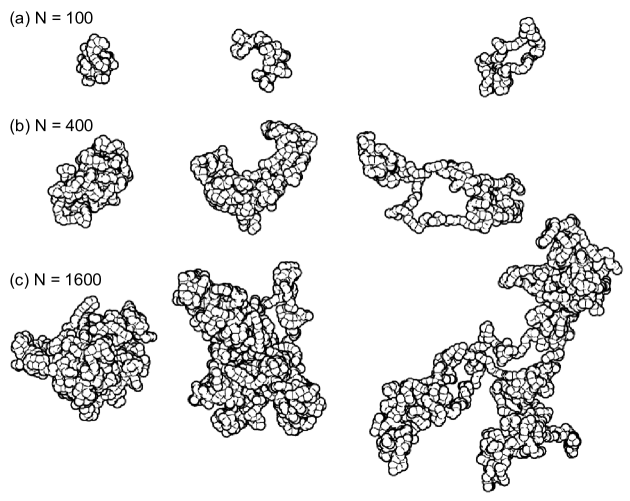
Figure 5: Individual chain snapshots for three of the ring systems. The left and right columns show small and large chains, respectively, while the middle column shows a chain having nearly the average value of $R_{g}^{2}$.

		Linear					Rings						Solid
	$m$	$N=100$	200	400	800	Gaussian	$N=100$	200	400	800	1600	Gaussian	Sphere
$R_{g}^{(4)}/R_{g}^{(2)}$	$2$	$1.18$	$1.18$	$1.19$	$1.18$	$1.19$	$1.13$	$1.14$	$1.14$	$1.15$	$1.15$	$1.14$	$1.04$
$R_{g}^{(6)}/R_{g}^{(2)}$	$3$	$1.34$	$1.35$	$1.36$	$1.36$	$1.36$	$1.24$	$1.26$	$1.27$	$1.28$	$1.28$	$1.25$	$1.07$
$R_{g}^{(8)}/R_{g}^{(2)}$	$4$	$1.48$	$1.50$	$1.51$	$1.52$	$1.53$	$1.35$	$1.36$	$1.38$	$1.40$	$1.41$	$1.36$	$1.10$
$R_{g}^{(10)}/R_{g}^{(2)}$	$5$	$1.61$	$1.64$	$1.65$	$1.67$	$1.67$	$1.44$	$1.46$	$1.49$	$1.51$	$1.52$	$1.46$	$1.11$

Table 3: Average higher moments of the single-chain distance distribution for the linear and ring systems as computed by Eq. 5. The values for a Gaussian linear chain and Gaussian ring are also given for comparison with the MD results. For a solid sphere $R_{g}^{(2m)}/R_{g}^{(2)}=(5/3)^{1/2}[3/(2m+3)]^{1/2m}$. Note that $\langle R_{g}^{2}\rangle^{1/2}=R_{g}^{(2)}$.

To illustrate this Fig. 5 shows three individual ring snapshots for each of the $N=100$, 400 and 1600 systems. Chains are taken from the wings and center of the distribution of $R_{g}$. The extensions increase from left to right with the chain in the middle chosen to have approximately $\left\langle R_{g}^{2}\right\rangle$. The smallest chains for each system are found to be collapsed while the largest are expanded and exhibit voids which are occupied by neighboring chains. This last point is confirmed by a primitive path analysis in the subsequent paperHalverson et al. (2011) and self-density data which is presented below. The conformations in the left and center columns of Fig. 5 are representative of the crumpled globule where each chain has a globule-like core surrounded by protrusions of size ${\cal O}(N_{e})$. The variety of conformations in Fig. 5 raises the point of whether there is a significant entropy barrier between the quasi-collapsed state of a ring and an extended conformation, which requires significant ring-ring interpenetration without concatenation. To illustrate that this barrier is very small or even nonexistent (as suggested by the unimodal distributions in Fig. 4a), Fig. 6 shows $R_{g}(t)$ and snapshots for three individual polymers from the $N=1600$ ring simulation. Chain 35 has a highly extended conformation with a large value of $R_{g}$ around $t=34.5\times 10^{6}~{}\tau$, however, $4.5\times 10^{6}~{}\tau$ later the chain is found to assume a less extended conformation with a corresponding reduction in $R_{g}$ of 50%. A similar behavior is found for chain 38 while the size of chain 51 remains at approximately the root-mean-square value (as indicated by the horizontal line) over the entire time window.

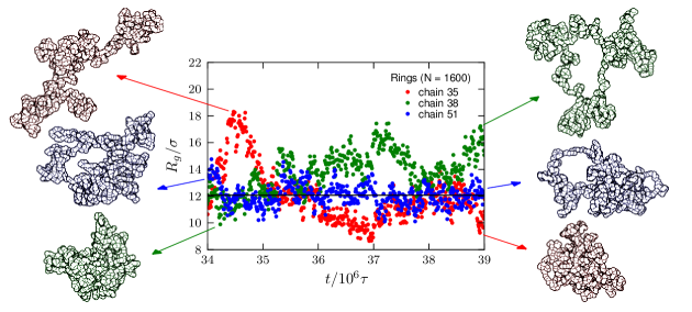
Figure 6: Radius of gyration for three individual chains from the $N=1600$ ring melt simulation as a function of time along with instantaneous configurations. The horizontal line indicates the value of $\left\langle R_{g}^{2}\right\rangle^{1/2}$.

The internal structure of the chains may be characterized by the mean-square internal distances. Let $[d(s)]^{2}$ denote the average squared distance between two monomers separated by $s$ bonds. This quantity normalized by $\langle R_{e}^{2}\rangle$ is shown in Fig. 7a. The local rigidity of the chains leads to an approximate $s^{2}$ scaling for short separations. An intermediate regime with a linear scaling in $s$ is found for $l_{k}/d(s=1)\ll s\ll N/2$, where $l_{k}$ is the Kuhn length which for our modelEveraers et al. (2004) is $2.79~{}\sigma$. The $[d(s)]^{2}\sim s$ behavior is found for linear chains where it is also the asymptotic scaling. For the rings at very large separations a $s^{2/3}$ regime is found before $[d(s)]^{2}$ becomes independent of $s$ as $s$ approaches half of the chain. In Fig. 7b the mean-square internal distances are normalized by those of a Gaussian ringZimm and Stockmayer (1949) or $\left\langle[d(s)]^{2}\right\rangle=l_{k}l/[1/s+1/(N-s)]$, where $l$ is the average bond length. Although the overall shape of the $d(s)$ dependence is quite reminiscent of that of a Gaussian ring, it is definitely not the same. Of course, this is not surprising because unlike linear chains, rings in the melt are not Gaussian.

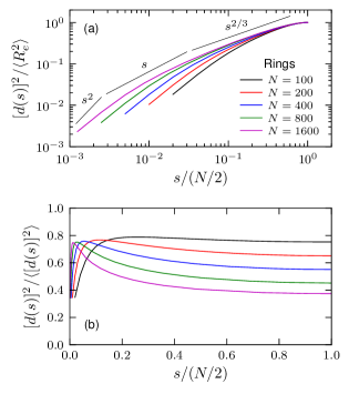
Figure 7: Internal structure of the rings as characterized by the mean-square internal distances normalized by (a) the mean-square spanning distance and (b) the scaling for a Gaussian ring or $\left\langle[d(s)]^{2}\right\rangle=l_{k}l/[1/s+1/(N-s)]$, where $s$ is the number of bonds separating two monomers and $1\leq s\leq N/2$. Normalizing by $\left\langle R_{e}^{2}\right\rangle$ in (a) causes all five data sets to coincide at $s=N/2$.

The static structure function of the individual rings multiplied by $q^{3}$ is shown in Fig. 8. For $2\pi/\left\langle R_{g}^{2}\right\rangle^{1/2}<q\ll 2\pi/l_{k}$ one expects $S(q)\sim q^{-1/\nu}$ for self-similar structures. While this scaling is almost perfectly fulfilled for linear chains with $\nu=1/2$, the situation is more complex for the rings. If the large rings behaved like homogeneous, compact objects then one would expect $S(q)$ to be dominated by Porod scatteringGrest et al. (1987, 1989) or $S(q)\sim q^{-4}$. This is certainly not the case here. The best fit to $S(q)\sim q^{-x}$ in this intermediate self-similar scaling regime is $x=3.2\pm 0.1$. This will be explained in a more general context in the discussion section. The inset of Fig. 8a shows $S(q)/N$ versus $q\left\langle R_{g}^{2}\right\rangle^{1/2}$. For large values of $q$ one finds a gradual increase in $S(q)q^{3}$ indicating a conformation between an overall collapsed, but very irregularly and self-similarly shaped object. All systems show a qualitatively self-similar behavior over a wide range of $q$ indicating that the general chain shape is the same between cases. The shift in the overall amplitude of $S(q)q^{3}$ in the intermediate regime, however, indicates that, unlike for linear chains, there is some deviation from the ideal fractal object structure, i.e. a weak ring length dependence of the density of scatterers.

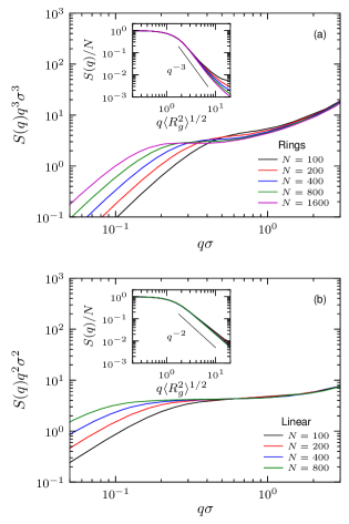
Figure 8: The single-chain static structure factor multiplied by (a) $q^{3}$ for the rings and (b) $q^{2}$ (Kratky plot) for the linear chains.

Taking the information revealed by Figs. 7 and 8, the apparently changing exponents from $\nu=1/2$ for very short rings to $\nu=1/3$ for the long ones can be seen as a crossover into the asymptotic regime without significant qualitative influence on the internal structure. Actually, one would expect each ring to have a fairly large number of surface beads ($n_{\mathrm{surf}}$), where a bead is a surface bead if it is within a distance $r$ of at least one bead of another chain. For random walks, i.e. linear melts, “all” beads (${\cal O}(N)$) are surface beads, while for a compact sphere only ${\cal O}(N^{2/3})$ are surface beads. For the rings we find $n_{\mathrm{surf}}\sim N^{\beta}$, $\beta\approx 0.95$ (see Fig. 9). This power law covers the whole range from $N=100$ to 1600 without any sign of a crossover. The observed exponent of $0.95$ is very close to unity, so one is inclined to suspect that in fact $n_{\mathrm{surf}}\sim N^{1}$, however, the data do suggest that this power is slightly below unity and there are also theoretical grounds to expect it to be smaller than 1.0 (see Appendix).

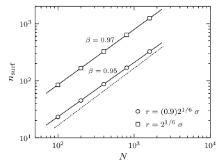
Figure 9: Number of surface monomers per chain versus $N$ for two choices of the cutoff distance as indicated. The error in values of $n_{\mathrm{surf}}$ is approximately 0.5%, significantly smaller than the symbol size, suggesting that the observed exponent can be distinguished from 1 (dashed line).

The internal structure of the chains can also be characterized by $P(s)$, which is the probability of two monomers of the same chain being separated by $s$ bonds and a distance of less than $r$. In Fig. 10, $P(s)$ is shown for the ring melts for the same two choices of the cutoff distance as in Fig. 9. For the larger rings one finds a power law of $P(s)\sim s^{-\gamma}$ for intermediate values of $s$. The value of $\gamma$ is found to decrease weakly with increasing $s$. For the larger cutoff distance and $N=1600$, $\gamma$ varies from 1.17 when the data is fit to values of $s$ between $30-50$ to 1.00 for values between $110-130$. The same trend is seen for the smaller value of $r$.

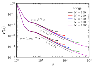
Figure 10: $P(s)$ is the probability of two monomers of the same chain being separated by $s$ bonds and a distance of less than $r$.

To finally confirm that the rings do not assume double-stranded conformations we computed the probability distribution function of the angle formed by vectors $\boldsymbol{a}=\boldsymbol{r}_{i+n}-\boldsymbol{r}_{i}$ and $\boldsymbol{b}=\boldsymbol{r}_{j+n}-\boldsymbol{r}_{j}$, where $\boldsymbol{r}_{k}$ is the position vector of monomer $k$ and $j>i$. The calculation was performed only when $|\boldsymbol{r}_{i}-\boldsymbol{r}_{j}|$ was less than a distance, $r$, which was taken as a multiple of the excluded-volume interaction cutoff and covered a range from nearest-neighbor separations to approximately the tube diameter ($2\left\langle R_{g}^{2}(N_{e})\right\rangle^{1/2}\approx 7~{}\sigma$) as based on the linear chain system. For all combinations of $n=1,2,3$ and $r/r_{c}=1,2,3,4,5$ the distribution function was found to be consistent with the vectors having random orientations confirming that rings in the melt are not double-stranded. Such a finding casts severe doubt on approaches which are based on lattice animal arguments.

Figure 11: Self-excluded monomer density profiles for the rings and linear systems. For (a) and (c), $r=0$ corresponds to the center-of-mass of the central chain while for (b) and (d) it corresponds to the center of maximum density.

The entropy loss associated with the nonconcatenation constraint suggests that a ring melt should have a higher pressure than a linear melt at the same density and temperature. This is supported by the finding that a single ring in a linear melt (where there is no concatenation constraint) has a larger size than in a melt of rings.Iyer et al. (2007) We can estimate the pressure contribution due to the restricted topology of nonconcatenated rings by following the ideas of Ref. 36. According to that work, entropy loss due to topological constraints is of the order of the number of rings contacting a given ring, the quantity called $K_{1}$ below. That corresponds to a contribution to the pressure which is of the order of $k_{B}TK_{1}/Nv$, where $Nv$ is the volume of a ring. Given that $k_{B}T=\epsilon$ (see Simulation Methodology section above), and $v\approx\sigma^{3}$, we arrive at the estimate of the pressure as $K_{1}/N$ in the units of $\epsilon/\sigma^{3}$. Given that $K_{1}$ is less than 20 (see below), we arrive for $N=800$ at the pressure contribution of less than $0.025~{}\epsilon/\sigma^{3}$. While this estimate is open for criticism, since it is based on the method of Ref. 36 which does not produce the correct scaling exponent in $\left\langle R_{g}\right\rangle\sim N^{\nu}$, the deviation is not so large that the total pressure would be significantly changed.

The above estimate of the topological contribution to the pressure is compared to the overall pressure which was measured by MD simulation and found to be $P=4.99\pm 0.02~{}\epsilon/\sigma^{3}$ for $N=800$. Thus, the estimated topological contribution is two orders of magnitude smaller than the pressure and is roughly the same magnitude as the error bars of our measurements. It is therefore not surprising that we obtained an indistinguishable pressure of $5.00\pm 0.01~{}\epsilon/\sigma^{3}$ for the melt of linear chains at the same conditions. Further work is required to detect the topological contribution to the pressure and examine its exact scaling behavior.

The overall properties of a single ring in the melt display the general scaling of a compact object. However, the conformations are open enough in order to allow for a significant interpenetration of rings. Such rather extended shapes require that the depth of the correlation hole, which measures the self-density of the chains, be significantly deeper than for linear melts. For linear polymers the volume of each chain is shared by $N^{1/2}$ other chains, resulting in a vanishing self-density of the chains, i.e. $\rho_{\mathrm{self}}\sim N^{-1/2}$. For a compact object, independent of the overall bead density, $\rho_{\mathrm{self}}$ eventually has to become independent of $N$. In Fig. 11 the self-excluded density profile is shown for the rings and linear chains. This profile is computed in the standard way for Figs. 11a,c except that the origin is taken as the center-of-mass of the central chain and the monomers of the central chain are ignored in the calculation. For each system the magnitude of $\rho_{\mathrm{ex}}$ in the vicinity of $r=0$ does not vanish. This arises from the mutual interpenetration of chains and is more pronounced for the linear. $\rho_{\mathrm{ex}}(r\rightarrow 0)$ is found to approach a constant for the longer rings ($N\geq 400$). For Figs. 11b,d the center of maximum density of the central chain is used. This is found by a binning procedure with a bin size of $5~{}\sigma$. The self-density as $r\rightarrow 0$ is shown in Fig. 12 where it can be seen that this quantity for the rings approaches a constant as $N\rightarrow\infty$.

Figure 12: Log-log plot of the self-density as $r\rightarrow 0$ multiplied by $N^{1/2}$ versus inverse chain length for the rings and linear polymers. $\rho_{\mathrm{self}}$ around the center-of-mass for linear polymers vanishes with $N^{-1/2}$ while for the rings it approaches a chain length independent constant of $\rho_{\mathrm{self}}(N\rightarrow\infty)\approx 0.31~{}\sigma^{-3}$. Note that $\rho_{\mathrm{self}}(r)=\rho-\rho_{\mathrm{ex}}(r)$.

The behavior of $\rho_{\mathrm{ex}}(r)$ is consistent with the observed decrease in self-density with increasing $N$, if estimated from $\left\langle R_{g}^{2}\right\rangle^{1/2}$. With the self-density being $\rho_{\mathrm{self}}=3N/4\pi\left\langle R_{g}^{2}\right\rangle^{3/2}$ (which assumes a homogeneous sphere), we find $\rho_{\mathrm{self}}=0.34~{}\sigma^{-3}$ for $N=100$ while for the large rings ($N\geq 400$) this value drops to around 0.23. Since the bulk density is $0.85~{}\sigma^{-3}$ this implies that roughly $70\%$ of the monomers within $\left\langle R_{g}^{2}\right\rangle^{1/2}$ of the center-of-mass of the long rings come from other chains. This, in combination with $\nu=1/3$ means that the number of different rings in direct contact with a given ring should asymptotically become independent of $N$.

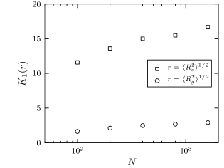
Figure 13: Number of neighboring chains versus $N$. $K_{1}(r)$ is the average number of chains within a center-of-mass separation distance $r$.

The structure of a polymer melt is partly determined by the number of neighbors per chain. Let $K_{1}(r)$ denote the average number of chains whose center-of-mass is within a distance $r$ of the center-of-mass of a reference chain. This quantity is shown in Fig. 13 as a function of $N$ for the rings. As chain length increases $K_{1}(r)$ approaches a constant for both $r=\left\langle R_{g}^{2}\right\rangle^{1/2}$ and $r=\left\langle R_{e}^{2}\right\rangle^{1/2}$, which is in agreement with our arguments above (i.e., as $N\rightarrow\infty$, $\nu\rightarrow 1/3$). This is to be contrasted with the fact that $K_{1}(\left\langle R_{g}^{2}\right\rangle^{1/2})$ for the melt of linear chains grows as $N^{1/2}$. This agrees with the finding that the rings in the melt, although collapsed overall, do have significant protrusions into one another. The lattice simulations of Vettorel et al. Vettorel et al. (2009) gave a limiting value of $K_{1}(\left\langle R_{g}\right\rangle)\approx 14$ as $N\to\infty$ which agrees well with the value of around 16 for the $N=1600$ system in the present work. This interplay of (partial) segregation and (partial) interpenetration is expected to play an important role for the dynamics of the melts, which is our focus in the following paper.

IV Discussion

While the linear chains show a $\left\langle R_{g}^{2}\right\rangle\sim N$ behavior for all chain lengths, the rings behave differently. While the conjecture of Cates and Deutsch Cates, M.E. and Deutsch, J.M. (1986) based on a free energy argument that the Flory exponent for the radius of gyration of a ring polymer melt should be approximately $2/5$ has reportedly been confirmed by a number of simulation Müller et al. (1996); Brown and Szamel (1998); Müller et al. (2000); Iyer et al. (2007); Vettorel et al. (2009); Suzuki et al. (2009) and theoretical Suzuki et al. (2009) studies, it now appears that this corresponds to an intermediate regime with the asymptotic Flory exponent being $1/3$ Müller et al. (2000); Vettorel et al. (2009); Suzuki et al. (2009). The present work is in agreement with the scaling laws for these two regimes. Vettorel et al. Vettorel et al. (2009) estimate the onset of the asymptotic regime using an argument based on $N_{e,\mathrm{linear}}$. For the scheme where chains form a core which squeezes out the other rings, these authors estimate a critical ring length $N_{c}$ to be

$$N_{c}\approx\rho(4\pi/3)\left\langle R_{e,\mathrm{linear}}^{2}(N_{e,\mathrm{linear}})\right\rangle^{3/2},$$ (6)

which in our case leads to $N_{c}\approx 2300$. Thus it is clear that even with our longest rings, which based on a comparison of the entanglement length for polystyrene would correspond to a molecular mass of more than $10^{6}$ g/mol, we only would observe the crossover towards the $\left\langle R_{g}^{2}\right\rangle\sim N^{2/3}$ scaling. While this estimate assumes that the rings squeeze each other out more or less completely, the data show that this is not the case. The incomplete segregation of rings, in which the self-density $\rho_{\mathrm{self}}$ is about $1/3$ of the bulk density inside any particular coil reduces the expected crossover chain length to $N_{c}\approx 700-800$ in good agreement with our data. This is actually a lower limit for $N_{c}$, since the crumpled globules are not ideal spherical objects, and it illustrates that one needs extremely long rings to unambiguously investigate the asymptotic regime.

Although rings in the melt appear to be compact objects in the sense that $\left\langle R_{g}^{2}\right\rangle\sim N^{2/3}$ at sufficiently large $N$, their compactness is of a non-trivial character. In many cases, they are torus (or even pretzel)-shaped; their higher moments are much larger than those of a solid sphere; and their average self-density, although it does not asymptotically depend on $N$, remains at roughly $\rho/3$ instead of $\rho$. These facts indicate that different rings in the melt, although reasonably segregated in the scaling sense, have nevertheless significant protrusions into one another. This can also be seen in the critical exponents describing the system.

In the familiar linear polymer coil, everything is governed by the single Flory exponent $\nu$, which describes the coil gyration radius. Although the rings in the melt appear to exhibit the asymptotic scaling $\left\langle R_{g}^{2}\right\rangle^{1/2}\sim N^{1/3}$, their properties are not completely determined by the value of the exponent ($\nu=1/3$), at least not in a trivial way. There are two important examples of exponents that are not directly related to $\nu$. The first describes the number of “surface monomers” (see above, Section III), i.e., monomers of a given polymer that have contacts with other polymers: $n_{\mathrm{surf}}\sim N^{\beta}$; we find that our simulations yield $\beta\approx 0.95$. We argue that the same power $\beta$ should describe the number of contacts between two crumples of $g$ monomers each, whether belonging to the same ring or to two different rings; this number of contacts scales as $g^{\beta}$. The second is the $\gamma$ exponent which describes the looping probability – the probability that two monomers of the same ring, a distance $s$ along the chain, will be found next to each other in space. The looping probability scales as $s^{-\gamma}$. Understanding this exponent for rings in the melt is of particular interest because this system, as mentioned in the introduction section, is expected to capture essential features of chromatin packing in chromosomes. The exponent $\gamma$ can be measured directly for chromatin using HiC methods Dekker et al. (2003); Simonis et al. (2006); Lieberman-Aiden et al. (2009); Duan et al. (2010). We now argue that there is a general scaling relation between exponents $\beta$ and $\gamma$, namely, $\beta+\gamma=2$ (see Appendix for derivation). Our simulation data, presented above (see Figs. 9 and 10) are closer to $\beta+\gamma\approx 2.1$. It is not completely clear to us whether this result agrees with the theoretical prediction to within the error bars of the simulation data, or the deviation is real. Uncertainty in the simulation data is thought to arise from finite size effects. Interestingly, the simulation result for $\gamma\approx 1.1$ is also close to the mean field prediction $\gamma=3\nu$ (see Appendix) as well as to the experimental result for chromatin Lieberman-Aiden et al. (2009) $\gamma\approx 1$. Thus, our current understanding is that $\beta$ is slightly smaller than unity, while $\gamma$ is slightly larger than unity. The former observation indicates that there are many contacts between crumples, but still not all of the monomers are in contact, i.e., there is some segregation between crumples; in terms of modeling the chromatin, this is consistent with the concept of chromosome territories Solovei et al. (2002). The later observation is also consistent with the idea that the system is a fractal. Indeed, a true fractal on an unlimited spectrum of scales cannot be realized with $\gamma\leq 1$ (because then the total number of contacts per monomer, proportional to $\sum_{1}^{N}s^{-\gamma}$ would diverge). Thus, the observed values of $\beta$ and $\gamma$ are consistent with the non-trivial segregated fractal structure.

The fact that we observe deviations from a generally expected $S(q)\sim q^{-1/\nu}$ scaling in the regime $2\pi/\left\langle R_{g}^{2}\right\rangle^{1/2}\ll q\ll 2\pi/\sigma$ as well as the finding $\beta<1$ can be rationalized by generalizing a recent investigation of 2-d polymer melts by Meyer et al.Meyer et al. (2010) Their analysis is based on a rather general theoretical framework of B. DuplantierDuplantier (1989). While the Duplantier theory applies in 2-d only, and no 3-d generalization is available (precisely because of the difficulties with topological constraints), the scaling considerations can be developed for our 3-d system in the following way. In a 2-d polymer melt the chains form compact objects and partially segregate. The situation here is somewhat similar and we can generalize this concept to our problem of a melt of nonconcatenated rings. In general, with $n$ scatterers (being the whole ring or just a part):

$$S(q)=\frac{1}{n}\left\langle\sum_{i,j=1}^{n}\exp[i\boldsymbol{q}\cdot(\boldsymbol{r}_{i}-\boldsymbol{r}_{j})]\right\rangle,$$ (7)

where one finds for $q\rightarrow 0,~{}S(q)\rightarrow n$. For the intermediate scaling regime, for a fractal structure one expects $S(q)\sim(q\left\langle R_{g}\right\rangle)^{-x}$. These two arguments imply $S(q)\sim n(q\left\langle R_{g}\right\rangle)^{-x}$ with $x$ to be determined. The total scattering intensity $I(q)=nS(q)$ for intermediate values of $q$ can only result from the beads at the surface of the ring polymer, as these are the only places where a scattering probe experiences a contrast. Consequently we expect $I(q)\sim n^{\beta}/q^{x}$. Combining all this leads to the scaling relation $2-x\nu=\beta$ or $x=(2-\beta)/\nu$ and a power law of

$$S(q)\sim n^{\beta-1}/q^{(2-\beta)/\nu}$$ (8)

in the intermediate scattering regime. For a random walk, where “all” beads are surface beads, $\beta=1$ and $\nu=1/2$, we recover the well known $q^{-2}$ power law for $S(q)$, which also is very well reproduced by our data. For the rings the situation is more complex. The best estimate for $\beta$ is 0.95 as shown in Fig. 9. This would lead to a small amplitude shift in $S(q)$ between $N=100$ and $N=1600$ of about $10-20\%$, which indeed is observed. In addition, with $\nu=1/3$ we find $(2-\beta)/\nu\approx 3.1-3.2$ also in good agreement with the data. Fig. 14 shows the scaling plot for $S(q)$ displaying the overall consistency of the data as well as the result that the best fit of $\beta$ for the scattering data is 0.93, which once again agrees with $\beta$ less than 1. Keeping in mind that very long rings are needed to reach the asymptotic regime makes a precise estimate of $\beta$ quite difficult. However, the overall consistency of $S(q)$ and the independent determination of $\beta$ strongly support the general scheme and $\beta<1$.

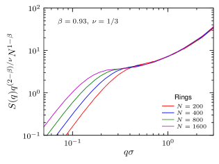
Figure 14: The single-chain static structure factor multiplied by the general scaling factor $q^{(2-\beta)/\nu}N^{1-\beta}$ with $\beta=0.93$ and $\nu=1/3$ for the rings with $N\geq 200$.

For linear chains longer than $N_{e,\mathrm{linear}}$, topological constraints manifest themselves in that a “tube defect” (one strand leaking out of its tube) becomes entropically unfavorable when the involved excursion reaches a length larger than $L_{e}=b\sqrt{N_{e,\mathrm{linear}}}$. In some form, similar behavior is expected in the case of rings as well. After the initial Gaussian-like scaling of very short chains, the lattice animal structure then emerges as the next natural conformation. However, this structure is restricted due to the same arguments, which make tube leakage very unfavorable. Any extended branch of a lattice animal would suffer from a severe entropy penalty. This restricts the average branch extension to a volume with a radius of approximately the tube diameter or to a chain length of about $2N_{e,\mathrm{linear}}$. Importantly, effective obstacles forcing the topological constraints are imposed not only by the surrounding chains, but also by the remote parts of the same chain. Unlike for a melt of linear chains, this is important for rings, because rings in the melt are compact and, therefore, the fraction of other pieces of the same chain among the spatial neighbors of any monomer is much higher in the ring system than in the linear melt. This eventually creates the crumpled globule conformation with rather small branches of size ${\cal O}(N_{e,\mathrm{linear}})$, bulging in and out at any place along the contour. A related lattice of obstacles model suggests that the nonconcatenated ring in the melt to some extent can be thought of as an annealed branched polymer. It is annealed in the sense that the material can move from one branch to another in the course of thermal motion, as Milner and Newhall have recently emphasized Milner and Newhall (2010). The important difference however is that, as the data nicely show, the densely-folded regions can open up and allow for significant interpenetration.

V Conclusions

Thus far we have presented a rather detailed study of the static properties of a melt of nonconcatenated rings. Even though asymptotically the ring extension follows a $N^{1/3}$ power law, suggesting that the rings have an overall globular conformation, their structure is far from trivial. Rings still display significant mutual interpenetration and the entropic barrier to form fairly large open loops is, in fact, so small that they are frequently observed. Though overall compact this leads to the fact that almost ${\cal O}(N)$ of the beads are surface beads. These structural peculiarities have important consequences for dynamics, as will be shown in the subsequent paperHalverson et al. (2011). Though already quite extensive, the current analysis leaves out many properties of relevance to biology, i.e. chromatin packing. Quantities specifically motivated by biological problems such as inter- and intra-ring contact maps will be studied in a separate publication.

Appendix A Relation between critical exponents of surface monomers and loop factor

The purpose of this appendix is to derive the relation between powers $\beta$ and $\gamma$, as mentioned in the section IV. To begin with, recall the definitions of these powers:

• Exponent $\gamma$ describes the loop factor, namely, the probability that two monomers a contour distance $s$ apart meet each other in space decays with $s$ as $s^{-\gamma}$.

• Exponent $\beta$ determines the number of “surface monomers”, $n_{\mathrm{surf}}\sim N^{\beta}$.

To derive the requisite relation between $\beta$ and $\gamma$, we start by noting that it is equally well applicable to the self-similar internal structure of any particular ring squeezed between other rings. In this latter case, exponent $\beta$ describes the number of monomer-monomer contacts between any two blobs, or crumples. Specifically, if two blobs are of some $g$ monomers each, and they are in contact (in the sense that the distance between them is about their own size), then the number of monomer-monomer contacts between them scales as $g^{\beta}$.

With this in mind, consider a ring in terms of $N/g$ blobs, $g$ monomers each. Concentrate on pairs of blobs which are a distance $s$ monomers, or $s/g$ blobs apart, along the chain. There are $N/g$ such pairs in the chain. Among these pairs some fraction are in contact. This fraction scales as a power of contour distance, i.e. it scales as $(s/g)^{-\gamma}$; therefore, the total number of blobs in contact is $(N/g)(s/g)^{-\gamma}=(N/s^{\gamma})g^{\gamma-1}$.

Now, let us consider monomer contacts instead of blob contacts. First, monomers are not in contact if they belong to non-contacting blobs. Second, given that there are $g^{\beta}$ monomer contacts per pair of contacting blobs, we can find the total number of contacts between monomers: $(N/s^{\gamma})g^{\gamma-1+\beta}$. Third, we have to realize that what we have counted is the number of contacting monomer pairs which are a distance $s\pm g$ along the chain. The number of monomer contacts a distance exactly $s$ apart is at least $g$ times smaller, i.e. $(N/s^{\gamma})g^{\gamma-2+\beta}$. Finally, the number of monomer contacts cannot depend on how we counted them, that is, it cannot depend on $g$. Therefore, we arrive at

$$\gamma+\beta=2.$$ (9)

As an example, consider a Gaussian polymer coil in 3-d. In this case, $\gamma=3/2$ and $\beta=1/2$, so formula (9) works. In general, for the Gaussian coil in $d$ dimensions, we have $\beta=2-d/2$ and $\gamma=d/2$, so again it works.

As mentioned in the main text, $\gamma>1$ is required for a mathematically rigorous fractal structure, which is self-similar over an infinite range of scales. This implies then that $\beta<1$; in this sense, different crumples of one chain or different rings must be segregated from each other, meaning that the number of “surface monomers” scales at least slower than the total $N$.

Although we have established the general relation between exponents $\beta$ and $\gamma$, theoretical determination of any one of them remains an open challenge. Mean field arguments suggest that for any fractal conformation with $r(s)\sim s^{\nu}$ in 3-d, the probability for two monomers to meet within a small volume $v$ should go as $v/r^{3}(s)\sim s^{-3\nu}$, which means $\gamma=3\nu$. This gives the familiar result $s^{-3/2}$ for the Gaussian coil, while for a crumpled globule this yields $s^{-1}$, i.e., an impossible $\gamma=1$. Of course, this only means the inapplicability of the mean field argument: monomers $s$ apart remain correlated in some yet unknown way instead of being independently distributed over the volume of the order of $r^{3}(s)$. Nevertheless, it is worth noting that $\gamma$ was found experimentally to be very close to unity for human chromosomes Lieberman-Aiden et al. (2009), while $\beta$ is found very close to unity in the present work. Clearly, $\gamma=1$ is impossible for a rigorous mathematical fractal, but it might be very close to unity for a real physical system which is only approximately self-similar even if over a very wide range of scales. It remains to be understood how all these facts are connected to each other.

References

- Halverson et al. (2011) J. D. Halverson, W. Lee, G. S. Grest, A. Y. Grosberg, and K. Kremer, J. Chem. Phys., DOI: 10.1063/1.3587138 (2011).
- de Gennes (1971) P. de Gennes, J. Chem. Phys., 55, 572 (1971).
- de Gennes (1979) P. de Gennes, Scaling Concepts in Polymer Physics (Cornell University Press, 1979).
- Doi and Edwards (1986) M. Doi and S. F. Edwards, The Theory of Polymer Dynamics (Oxford University Press, 1986).
- Tobolsky (1960) A. V. Tobolsky, Properties and Structure of Polymers (Wiley, New York, 1960).
- Onogi et al. (1970) S. Onogi, T. Masuda, and K. Kitagawa, Macromolecules, 3, 109 (1970).
- Berry and Fox (1968) G. C. Berry and T. G. Fox, Adv. Polym. Sci., 5, 261 (1968).
- Casale et al. (1971) A. Casale, R. S. Porter, and J. F. Johnson, J. Macromol. Sci. Rev. Macromol. Chem., C5, 387 (1971).
- Odani et al. (1972) H. Odani, N. Nemoto, and M. Kurata, Bull. Inst. Chem. Res. Kyoto Univ., 50, 117 (1972).
- Kremer and Grest (1990) K. Kremer and G. S. Grest, J. Chem. Phys., 92, 5057 (1990).
- Binder (1995) K. Binder, Monte Carlo and Molecular Dynamics Simulations in Polymer Science (Oxford University Press, 1995).
- McLeish (2002) T. C. B. McLeish, Advances in Physics, 51, 1379 (2002).
- Everaers et al. (2004) R. Everaers, S. K. Sukumaran, G. S. Grest, C. Svaneborg, A. Sivasubramanian, and K. Kremer, Science, 303, 823 (2004).
- Grosberg et al. (1988) A. Y. Grosberg, S. K. Nechaev, and E. I. Shakhnovich, Journal de Physique (France), 49, 2095 (1988).
- Bohn et al. (2010) M. Bohn, D. W. Heermann, O. Lourenço, and C. Cordeiro, Macromolecules, 43, 2564 (2010).
- Lua et al. (2004) R. Lua, A. L. Borovinskiy, and A. Y. Grosberg, Polymer, 45, 717 (2004).
- Cremer and Cremer (2001) T. Cremer and C. Cremer, Nature Reviews Genetics, 2, 292 (2001).
- Cremer et al. (2006) T. Cremer, M. Cremer, S. Dietzel, S. Müller, I. Solovei, and S. Fakan, Current Opinion in Cell Biology, 18, 307 (2006).
- Meaburn and Misteli (2007) K. J. Meaburn and T. Misteli, Nature, 445, 379 (2007).
- Vettorel et al. (2009) T. Vettorel, A. Y. Grosberg, and K. Kremer, Physics Today, 62, 72 (2009a).
- Vettorel et al. (2009) T. Vettorel, A. Y. Grosberg, and K. Kremer, Phys. Biol., 6, 025013 (2009b).
- Blackstone et al. (2011) T. Blackstone, R. Scharein, B. Borgo, R. Varela, Y. Diao, and J. Arsuaga, Journal of Mathematical Biology, 62, 371 (2011).
- Dorier and Stasiak (2009) J. Dorier and A. Stasiak, Nucleic Acids Research, 37, 6316 (2009).
- Sikorav and Jannink (1994) J.-L. Sikorav and G. Jannink, Biophysical Journal, 66, 827 (1994).
- Rosa and Everaers (2008) A. Rosa and R. Everaers, PLoS Computational Biology, 4, e1000153 (2008).
- Vettorel and Kremer (2010) T. Vettorel and K. Kremer, Macromolecular Theory and Simulations, 19, 44 (2010).
- Duan et al. (2010) Z. Duan, M. Andronescu, K. Schutz, S. McIlwain, Y. J. Kim, C. Lee, J. Shendure, S. Fields, C. A. Blau, and W. S. Noble, Nature, 465, 363 (2010).
- Therizols et al. (2010) P. Therizols, T. Duong, B. Dujon, C. Zimmer, and E. Fabre, Proceedings of the National Academy of Sciences, 107, 2025 (2010).
- Solovei et al. (2002) I. Solovei, A. Cavallo, L. Schermelleh, F. Jaunin, C. Scasselati, D. Cmarko, C. Cremer, S. Fakan, and T. Cremer, Experimental Cell Research, 276, 10 (2002).
- Dekker et al. (2003) J. Dekker, K. Rippe, M. Dekker, and N. Kleckner, Science, 295, 1306 (2003).
- Simonis et al. (2006) M. Simonis, P. Klous, E. Splinter, Y. Moshkin, R. Willemsen, E. de Wit, B. van Steensel, and W. de Laat, Nature Genetics, 38, 1348 (2006).
- Lieberman-Aiden et al. (2009) E. Lieberman-Aiden, N. L. van Berkum, L. Williams, M. Imakaev, T. Ragoczy, A. Telling, I. Amit, B. R. Lajoie, P. J. Sabo, M. O. Dorschner, R. Sandstrom, B. Bernstein, M. A. Bender, M. Groudine, A. Gnirke, J. Stamatoyannopoulos, L. A. Mirny, E. S. Lander, and J. Dekker, Science, 326, 289 (2009).
- Grosberg et al. (1993) A. Y. Grosberg, Y. Rabin, S. Havlin, and A. Neer, Europhysics Letters, 23, 373 (1993).
- Rosa et al. (2010) A. Rosa, N. B. Becker, and R. Everaers, Biophysical Journal, 98, 2410 (2010).
- Bancaud et al. (2010) A. Bancaud, C. Lavelle, S. Huet, and J. Ellenberg, (2010).
- Cates, M.E. and Deutsch, J.M. (1986) Cates, M.E. and Deutsch, J.M., Journal de Physique (France), 47, 2121 (1986).
- Khokhlov and Nechaev (1985) A. Khokhlov and S. Nechaev, Physics Letters A, 112, 156 (1985), ISSN 0375-9601.
- Rubinstein (1986) M. Rubinstein, Phys. Rev. Lett., 57, 3023 (1986).
- Nechaev et al. (1987) S. K. Nechaev, A. N. Semenov, and M. K. Koleva, Physica A: Statistical and Theoretical Physics, 140, 506 (1987).
- Obukhov et al. (1994) S. P. Obukhov, M. Rubinstein, and T. Duke, Phys. Rev. Lett., 73, 1263 (1994).
- Hild et al. (1983) G. Hild, C. Strazielle, and P. Rempp, Eur. Polym. J., 19, 1983 (1983).
- Roovers and Toporowski (1983) J. Roovers and P. M. Toporowski, Macromolecules, 16, 843 (1983).
- McKenna et al. (1987) G. B. McKenna, G. Hadziioannou, P. Lutz, G. Hild, C. Strazielle, C. Straupe, and P. Rempp, Macromolecules, 20, 498 (1987).
- Roovers and Toporowski (1988) J. Roovers and P. M. Toporowski, J. Polym. Sci. B, 26, 1251 (1988).
- Pasch and Trathnigg (1997) H. Pasch and B. Trathnigg, HPLC of Polymers (Springer, 1997).
- Lee et al. (2000) H. C. Lee, H. Lee, W. Lee, T. Chang, and J. Roovers, Macromolecules, 33, 8119 (2000).
- Kapnistos et al. (2008) M. Kapnistos, M. Lang, D. Vlassopoulos, W. Pyckhou-Hintzen, D. Richter, D. Cho, T. Chang, and M. Rubinstein, Nature Materials, 7, 997 (2008).
- (48) J. D. Halverson, G. S. Grest, A. Y. Grosberg, and K. Kremer, In preparation.
- Nam et al. (2009) S. Nam, J. Leisen, V. Breedveld, and H. W. Beckham, Macromolecules, 42, 3121 (2009).
- Müller et al. (1996) M. Müller, J. P. Wittmer, and M. E. Cates, Phys. Rev. E, 53, 5063 (1996).
- Brown and Szamel (1998) S. Brown and G. Szamel, J. Chem. Phys., 108, 4705 (1998a).
- Müller et al. (2000) M. Müller, J. P. Wittmer, and J.-L. Barrat, Europhys. Lett., 52, 406 (2000a).
- Brown and Szamel (1998) S. Brown and G. Szamel, J. Chem. Phys., 109, 6184 (1998b).
- Müller et al. (2000) M. Müller, J. P. Wittmer, and M. E. Cates, Phys. Rev. E, 61, 4078 (2000b).
- Brown et al. (2001) S. Brown, T. Lenczycki, and G. Szamel, Phys. Rev. E, 63, 052801 (2001).
- Suzuki et al. (2008) J. Suzuki, A. Takano, and Y. Matsushita, J. Chem. Phys., 129, 034903 (2008).
- Vettorel et al. (2009) T. Vettorel, S. Y. Reigh, D. Y. Yoon, and K. Kremer, Macromol. Rapid. Commun., 30, 345 (2009c).
- Suzuki et al. (2009) J. Suzuki, A. Takano, T. Deguchi, and Y. Matsushita, J. Chem. Phys., 131, 144902 (2009).
- Carmesin and Kremer (1988) I. Carmesin and K. Kremer, Macromolecules, 21, 2819 (1988).
- Hur et al. (2006) K. Hur, R. G. Winkler, and D. Y. Yoon, Macromolecules, 39, 3975 (2006).
- Tsolou et al. (2010) G. Tsolou, N. Stratikis, C. Baig, P. S. Stephanou, and V. G. Mavrantzas, Macromolecules, 43, 10692 (2010).
- Hur et al. (2011) K. Hur, C. Jeong, R. G. Winkler, N. Lacevic, R. H. Gee, and D. Y. Yoon, Macromolecules (2011).
- Pütz et al. (2000) M. Pütz, K. Kremer, and G. S. Grest, Europhys. Lett., 49, 735 (2000).
- Auhl et al. (2003) R. Auhl, R. Everaers, G. S. Grest, K. Kremer, and S. J. Plimpton, J. Chem. Phys., 119, 12718 (2003).
- Schneider and Stoll (1978) T. Schneider and E. Stoll, Phys. Rev. B, 17, 1302 (1978).
- Limbach et al. (2006) H. J. Limbach, A. Arnold, B. A. Mann, and C. Holm, Computer Physics Communications, 174, 704 (2006).
- Plimpton (1995) S. J. Plimpton, J. Comp. Phys., 117, 1 (1995).
- Wittmer et al. (2004) J. P. Wittmer, H. Meyer, J. Baschnagel, A. Johner, S. Obukhov, L. Mattioni, M. Müller, and A. N. Semenov, Phys. Rev. Lett., 93, 147801 (2004).
- Wittmer et al. (2007) J. P. Wittmer, P. Beckrich, H. Meyer, A. Cavallo, A. Johner, and J. Baschnagel, Phys. Rev. E, 76, 011803 (2007).
- Jagodzinski et al. (1992) O. Jagodzinski, E. Eisenriegler, and K. Kremer, J. de Physique I, 2, 2243 (1992).
- Zimm and Stockmayer (1949) B. H. Zimm and W. H. Stockmayer, J. Chem. Phys., 17, 1301 (1949).
- Grest et al. (1987) G. S. Grest, K. Kremer, and T. A. Witten, Macromolecules, 20, 1376 (1987).
- Grest et al. (1989) G. S. Grest, K. Kremer, S. T. Milner, and T. A. Witten, Macromolecules, 22, 1904 (1989).
- Iyer et al. (2007) B. Iyer, A. K. Lee, and S. Shanbhang, Macromolecules, 40, 5995 (2007).
- Meyer et al. (2010) H. Meyer, J. P. Wittmer, T. Kreer, A. Johner, and J. Baschnagel, J. Chem. Phys., 132, 184904 (2010).
- Duplantier (1989) B. Duplantier, J. Stat. Phys., 54, 581 (1989).
- Milner and Newhall (2010) S. T. Milner and J. D. Newhall, Phys. Rev. Lett., 105, 208302 (2010).