Multiple adaptive substitutions during evolution in novel environments

Running head: Adaptive walk in novel environment

Keywords: adaptive walk, walk length, fitness landscapes, extreme value theory

Corresponding author:
Kavita Jain,
Theoretical Sciences Unit and Evolutionary and Organismal Biology Unit,
Jawaharlal Nehru Centre for Advanced Scientific Research,
Jakkur P.O., Bangalore 560064, India.
jain@jncasr.ac.in

Abstract: We consider an asexual population under strong selection-weak mutation conditions evolving on rugged fitness landscapes with many local fitness peaks. Unlike the previous studies in which the initial fitness of the population is assumed to be high, here we start the adaptation process with a low fitness corresponding to a population in a stressful novel environment. For generic fitness distributions, using an analytic argument we find that the average number of steps to a local optimum varies logarithmically with the genotype sequence length and increases as the correlations among genotypic fitnesses increase. When the fitnesses are exponentially or uniformly distributed, using an evolution equation for the distribution of population fitness, we analytically calculate the fitness distribution of fixed beneficial mutations and the walk length distribution.

Adaptation is an evolutionary process during which a population improves its fitness by accumulating beneficial mutations. A population of genotypic sequences produces a suite of mutants and if better mutants become available, a maladapted population may acquire one of the beneficial mutations provided it does not get lost due to genetic drift. The fitter population in turn may acquire another advantageous mutation and the process goes on until the supply of beneficial mutations gets exhausted. A number of models with variable degrees of biological consistency have been proposed and investigated to understand the process of adaptation (Miller et al., 2011). One of the simplest mathematical models was introduced by Gillespie in which beneficial mutations arise sequentially and fix rapidly (Gillespie, 1991). If the mutation rate is small and the selection coefficient is large (compared to the inverse population size), it is a good approximation to assume that only the one-step mutants are accessible at any time and the population is localised at a single genotype. Such a monomorphic population performs an adaptive walk by moving uphill on a fitness landscape until no more beneficial mutations can be found.

In the last few years, much of the work on Gillespie’s model has focused on the first step in the adaptation process. If the fitness of the wild type and its one-mutant neighbors are rank ordered with the fittest sequence at the top, the well established theory of extremes of independent random variables (David and Nagaraja, 2003) can be exploited to obtain useful information provided the wild type has a high fitness (rank). For a moderately high ranked initial fitness, Orr calculated the expected rank at the first step assuming exponential-like fitness distributions (Orr, 2002). His prediction has been tested in an experiment using single-stranded DNA and found to be roughly consistent with the experimental data (Rokyta et al., 2005). This result has been later generalised for other fitness distributions (Joyce et al., 2008) and by including correlations among fitnesses (Orr, 2006). However as the properties of the entire walk are required to design a drug or a biomolecule (Bull and Otto, 2005) and as experimental data on multiple adaptive substitutions is becoming available (Rokyta et al., 2009; Schoustra et al., 2009), it is important to extend the existing theory to address the statistical properties of the entire walk.

With this aim, we study Gillespie’s mutational landscape model on rugged fitness landscapes with many local fitness optima. An important difference between our work and the previous ones is that here we start the adaptive walk with low fitness to describe the adaptation process in novel environments such as when antibiotics are introduced (MacLean and Buckling, 2009; McDonald et al., 2010) whereas the initial fitness is assumed to be high in other studies (Gillespie, 1991; Orr, 2002, 2006; Joyce et al., 2008). Several numerical (Gillespie, 1991; Orr, 2006) and experimental studies (Rokyta et al., 2009; Schoustra et al., 2009) have indicated that only a few steps are required to reach a local optimum. In a simple adaptation model that assumes the mutational neighborhood to remain unchanged during the entire adaptive walk (Gillespie, 1983), the average number of steps to a local fitness peak has been calculated analytically for various fitness distributions and shown to increase logarithmically with the rank of the initial sequence (Neidhart and Krug, 2011). However here we work with a more realistic mutation scheme in which a new suite of mutants is created in each adaptive step. For generic fitness distributions, we argue that the average number of adaptive steps increases logarithmically with sequence length with a prefactor that depends on the choice of fitness distribution. Although our argument does not capture the proportionality constant correctly, the logarithmic dependence is seen to be in excellent agreement with the simulation results. We also present detailed results on the statistical properties of entire walk for exponentially and uniformly distributed fitnesses as these two distributions lend themselves to an analytic treatment and are also consistent with the experiments (Eyre-Walker and Keightley, 2007; Rokyta et al., 2008). Following the approach of Flyvbjerg and Lautrup (1992), we write a recursion relation for the fitness distribution of fixed beneficial mutations at an adaptive step which is valid for long sequences and fitness distributions with a finite mean. A similar distribution has been calculated in the clonal interference regime in which multiple mutants are produced per generation (Rozen et al., 2002) while here we work in the weak mutation regime. For the above mentioned distributions, we also find the distribution of walk length. The average walk length calculated using this approach gives a prefactor consistent with the numerical results.

Although for most of the article we work with uncorrelated fitnesses and assume that the distribution of the fitness does not change during the course of evolution, the effect of correlations is also discussed. As experiments support an intermediate degree of correlations in fitness landscapes (Carneiro and Hartl, 2010; Miller et al., 2011) and changing fitness distributions may be modeled by correlated fitnesses (Orr, 2006), we calculate the average number of steps to an optimum on a fitness landscape generated by the block model of correlated fitnesses in which a sequence is divided into several independent blocks and correlations arise when two sequences share some blocks (Perelson and Macken, 1995). The average walk length has been measured using numerical simulations in a block model in Orr (2006) and it was speculated that the average number of adaptive steps is independent of the underlying fitness distribution and increases linearly with the number of blocks. We show that while the latter result is roughly correct, the average number of steps to a local optimum is not independent of the fitness distribution which is a consequence of the result discussed above for the uncorrelated fitness landscapes.

MODELS AND METHODS

Uncorrelated and correlated fitness landscapes: An uncorrelated fitness landscape can be generated by assigning a fitness to a sequence independent of that of other sequences. The fitnesses are sampled from a common distribution $p(f)$ with support on the interval $[l,u]$. Although the full distribution of absolute fitness is unknown, one can obtain an insight into its nature through the distribution of beneficial mutations which has been measured in several theoretical and experimental studies (Eyre-Walker and Keightley, 2007). A theoretical argument suggests that since good mutations are rare, their distribution is governed by the upper tail of the fitness distribution $p(f)$ (Gillespie, 1991). It is known from the extreme value theory (EVT) for independent and identically distributed (i.i.d.) random variables that the asymptotic distribution of the extreme value can be one of the following three types (David and Nagaraja, 2003): Fréchet for algebraically decaying underlying distributions, Gumbel for unbounded distributions decaying faster than a power law and Weibull for bounded distributions. In order to be consistent with this result, we make the following choices for the fitness distributions:

$$p(f)= (\delta-1)(1+f)^{-\delta}~{} \delta>2$$ ,           (Fréchet) (1)

$$p(f)= \gamma f^{\gamma-1}e^{-f^{\gamma}}~{} \gamma>0$$ ,           (Gumbel) (2)

$$p(f)= \nu(1-f)^{\nu-1}~{} \nu>0,f<1$$ ,   (Weibull) (3)

The condition $\delta>2$ in (1) is imposed to keep the transition rate (6) finite (as explained later). The last two fitness functions (2) and (3) are of particular interest as several experimental results on the distribution of beneficial mutations have been found to lie in the Gumbel domain (Imhof and Schlotterer, 2001; Sanjuán et al., 2004; Rokyta et al., 2005; Kassen and Bataillon, 2006; MacLean and Buckling, 2009) and a recent work finds a best fit for the distribution of beneficial effects to a uniform distribution which lies in the Weibull domain (Rokyta et al., 2008).

We also study adaptive walks on correlated fitness landscapes which are generated using a block model (Perelson and Macken, 1995) in which a sequence of length $L$ is divided into $B$ blocks of equal size $L_{B}=L/B$. The block fitness is an i.i.d. random variable chosen from the distribution $p(f)$ and the sequence fitness is obtained on averaging over the fitnesses of the blocks in the sequence. If two sequences share one or more block, their fitnesses are correlated. The correlations can be tuned by changing the number of blocks: If the number of blocks $B=1$, sequence fitnesses are completely uncorrelated while $B=L$ gives strongly correlated fitnesses. It should be noted that the extreme value distribution of correlated fitnesses may change from the corresponding i.i.d. class even if correlations are weak (Jain et al., 2009; Jain, 2011). In the following discussion, we assume that the sequence fitnesses are uncorrelated and deal with the correlated fitnesses in the last subsection of this section.

Adaptive walk model for long sequences: We work with haploid binary sequences of length $L$ in the strong selection-weak mutation (SSWM) regime. If $N$ is the population size, the SSWM regime corresponds to $Ns\gg 1,N\mu\ll 1$ where $s$ is the selection coefficient and $\mu$ is the mutation probability per locus per generation. Since the expected number of mutants produced per generation is much smaller than one, mutations occur sequentially and double and higher mutations may be neglected. Thus the mutational neighbourhood of a sequence is limited to $L$ mutants which are single mutation away from it. If the fitnesses of the wild type sequence and its $L$ one-mutant neighbors are arranged in a descending order with the best fitness assigned the rank $1$, the transition probability that the population moves from the wild type with fitness rank $i$ and value $f_{i}$ to a mutant with rank $j<i$ and value $f_{j}$ is proportional to the fixation probability which is well approximated by $2(f_{j}-f_{i})/f_{i}$ in the strong selection limit (Gillespie, 1991). The normalised transition probability from fitness $f_{i}$ to fitness $f_{j}$ is given by

$$T(f_{j}\leftarrow f_{i})=\frac{f_{j}-f_{i}}{\sum_{k=1}^{i-1}f_{k}-f_{i}}~{},~{}1\leq j\leq i-1$$ (4)

Once the population has moved to a mutant sequence with fitness $f_{j}$ with probability $T(f_{j}\leftarrow f_{i})$, it produces a set of new mutants which are rank ordered and chosen according to (4) and the process repeats itself until the population reaches a local optimum whose nearest neighbors are all less fit than itself. Note that the parameters $N$ and $\mu$ have dropped out of the picture and the properties of the model depend on the sequence length (or the initial rank) and the distribution of sequence fitnesses.

The model described above has been studied using (4) and EVT in previous works (Gillespie, 1991; Orr, 2002, 2006; Joyce et al., 2008) assuming the initial fitness to be high (small $i$). In contrast, we start with a low fitness and write a recursion relation for the probability $P_{J}(f)$ that an adaptive walk has at least $J$ steps and the fitness is $f$ at the $J$th step, following Flyvbjerg and Lautrup (1992) who studied this distribution for random adaptive walks (see Appendix A). In the following discussion, it is assumed that the sequence length is large which allows the following two simplifications: first, the events in which a sequence is backtracked can be ignored and second, the transition rates can be written in terms of absolute fitnesses instead of fitness ranks. Consider a population at the $J$th adaptive step and with fitness $h$. It can proceed to the next step provided at least one fitter mutant is available. If $q(h)=\int_{l}^{h}dg~{}p(g)$, this event occurs with a probability $1-q^{L}(h)$ where it is assumed that at each step in the evolutionary process, $L$ novel mutants are available which have not been encountered before. While this is true at the first step, the number of novel mutants is $L-1$ at the second step since one of the mutants is the parent sequence itself which is not an allowed descendant as the walk always proceeds uphill. In fact for any $J\geq 2$, some of the mutants have already been probed but the error introduced by ignoring this complication is of the order of $1/L$ which is negligible for large $L$ (Flyvbjerg and Lautrup, 1992). Then for long sequences we can write

$$P_{J+1}(f)=\int_{l}^{f}dh~{}p(f)T(f\leftarrow h)~{}(1-q^{L}(h))P_{J}(h)~{},~{}J\geq 0$$ (5)

where $p(f)T(f\leftarrow h)$ gives the probability that a mutant with fitness $f>h$ is chosen. Furthermore for large $L$, it is a good approximation to replace the sum in the denominator of (4) by an integral and we may write

$$T(f\leftarrow h)=\frac{f-h}{\int_{h}^{u}dg~{}(g-h)~{}p(g)}~{},~{}f>h$$ (6)

Thus we work with absolute fitnesses instead of fitness ranks. Since the transition probability (6) is undefined for slowly decaying fitness distributions $p(f)\sim f^{-\delta}~{},~{}\delta\leq 2$, we restrict $\delta>2$ in (1). Using (6) in (5), we finally obtain

$$P_{J+1}(f)=\int_{l}^{f}dh~{}\frac{(f-h)p(f)}{\int_{h}^{u}dg~{}(g-h)~{}p(g)}~{}(1-q^{L}(h))P_{J}(h)~{},~{}J\geq 0$$ (7)

Equation (7) is the central equation of this article and we will employ it to obtain various results on the statistical properties of adaptive walks. In the following, we assume the initial condition $P_{0}(f)=\delta(f)$ corresponding to zero initial fitness. As $P_{J}(f)$ obeys an integral equation which are harder to analyse, we may try to write a differential equation for $P_{J}(f)$. Differentiating (7) with respect to $f$, we get:

$$P^{\prime}_{J+1}(f) = \int_{l}^{f}dh~{}\frac{(f-h)p^{\prime}(f)+p(f)}{\int_{h}^{u}dg~{}(g-h)~{}p(g)}~{}(1-q^{L}(h))P_{J}(h)~{},~{}J\geq 0$$ (8)

$$P^{{}^{\prime\prime}}_{J+1}(f) = \int_{l}^{f}dh~{}\frac{(f-h)p^{\prime\prime}(f)+2p^{\prime}(f)}{\int_{h}^{u}dg~{}(g-h)~{}p(g)}(1-q^{L}(h))P_{J}(h)$$ (9)

$$+ \frac{p(f)(1-q^{L}(f))}{\int_{f}^{u}dg~{}(g-f)~{}p(g)}P_{J}(f)~{},~{}J\geq 1$$

where prime denotes a $f$-derivative. On using (7) and (8) in (9), we find

$$P^{{}^{\prime\prime}}_{J+1}(f) = 2\frac{p^{\prime}(f)}{p(f)}P^{\prime}_{J+1}(f)+\left[\frac{p^{\prime\prime}(f)}{p(f)}-2\left(\frac{p^{\prime}(f)}{p(f)}\right)^{2}\right]P_{J+1}(f)$$ (10)

$$+ \frac{p(f)(1-q^{L}(f))}{\int_{f}^{u}dg~{}(g-f)~{}p(g)}P_{J}(f)~{},~{}J\geq 1$$

The first derivative term in the above equation can be eliminated by writing $P_{J}(f)=p(f){\tilde{P}}_{J}(f)$ which finally yields

$${\tilde{P}}^{{}^{\prime\prime}}_{J+1}(f)=\frac{p(f)(1-q^{L}(f))}{\int_{f}^{u}dg~{}(g-f)~{}p(g)}{\tilde{P}}_{J}(f)~{},~{}J\geq 1$$ (11)

In this article, we will restrict our attention to exponentially and uniformly distributed fitnesses as these two fitness distributions are consistent with the available empirical data. We show that due to (11), a second order ordinary differential equation is obeyed by a generating function of $P_{J}(f)$ for these two distributions which can be solved within an approximation subject to the following boundary conditions:

$$P_{J}(f)|_{f=l} = 0~{},~{}J\geq 1$$ (12)

$$P^{\prime}_{J}(f)|_{f=l} = \frac{p(l)}{\int_{l}^{u}dg~{}g~{}p(g)}~{}\delta_{J,1}$$ (13)

where (12) is a direct consequence of (7) and the equation (13) arises on using the initial condition in (8).

Besides $P_{J}(f)$, we also find the walk length distribution $Q_{J}$ and the average fitness ${\bar{f}}_{J}$ at the $J$th step which can be related to $P_{J}(f)$ as explained below. Integrating over $f$ on both sides of (7), we get

$$P_{J+1} = \int_{l}^{u}df~{}P_{J+1}(f)$$ (14)

$$= \int_{l}^{u}dh\int_{h}^{u}df~{}\frac{(f-h)p(f)}{\int_{h}^{u}dg(g-h)p(g)}~{}(1-q^{L}(h))P_{J}(h)$$ (15)

$$= \int_{l}^{u}dh~{}(1-q^{L}(h))P_{J}(h)=P_{J}-\int_{l}^{u}dh~{}q^{L}(h)P_{J}(h)$$ (16)

Then the walk length probability $Q_{J}$ that exactly $J$ steps are taken is given by

$$Q_{J}=P_{J}-P_{J+1}=\int_{l}^{u}dh~{}q^{L}(h)P_{J}(h)$$ (17)

with $Q_{0}=0$ since the initial fitness is zero. The above equation has a simple interpretation: Since $P_{J}(h)$ is the probability that at least $J$ steps are taken and the fitness at the $J$th step is $h$, exactly $J$ steps will be taken if all the $L$ mutants of the sequence at the $J$th step carry a fitness smaller than $h$ from which (17) follows. The average walk length ${\bar{J}}=\sum_{J=0}^{2^{L}}JQ_{J}\approx\sum_{J=0}^{\infty}JQ_{J}$ for large $L$. The average fitness ${\bar{f}}_{J}$ is defined as ${\bar{f}}_{J}=\int_{l}^{u}df~{}fP_{J}(f)$. Using (7), we can write

$${\bar{f}}_{J+1} = \int_{l}^{u}dff\int_{l}^{f}dh~{}\frac{(f-h)p(f)}{\int_{h}^{u}dg(g-h)p(g)}~{}(1-q^{L}(h))P_{J}(h)$$ (18)

$$= \int_{l}^{u}dh\frac{(1-q^{L}(h))P_{J}(h)}{\int_{h}^{u}dg(g-h)p(g)}\int_{h}^{u}dff(f-h)p(f)$$ (19)

Note that neither (17) nor (19) are closed equations.

Our analytical results are also compared with numerical simulations which were performed using an exact procedure for $L\leq 10$ and an approximate method outlined in Orr (2002) for larger $L$. We refer the reader to Appendix B for details.

RESULTS

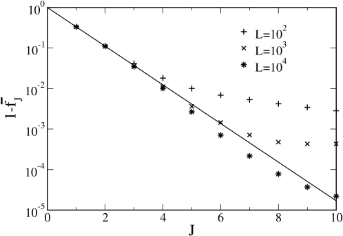
Figure 1: Evolution of average fitness with the number of adaptive steps starting from zero initial fitness obtained numerically (points) and compared with the average fitness in infinite sequence length limit (lines) for (a) power law distributed fitness with $\delta=6$, equation (22) (b) exponentially, equation (23) and (c) uniformly distributed fitness, equation (25).

Average fitness and walk length for general fitness distributions: For a broad class of fitness distributions, the average fitness for an infinitely long sequence can be computed. Although this limit is biologically unrealistic, it provides a good approximation to the average fitness ${\bar{f}}_{J}$ for small $J$ (see Fig. 1) as the population can not sense the finiteness of sequence length far from the local optimum. On taking the limit $L\to\infty$ in (19) and denoting the average fitness in this limit by $F_{J}$, we obtain

$$F_{J+1}=\int_{l}^{u}dh~{}\frac{\int_{h}^{u}df~{}f(f-h)p(f)}{\int_{h}^{u}dg~{}(g-h)p(g)}~{}P_{J}(h)|_{L\to\infty}$$ (20)

Algebraically decaying fitness distributions: On substituting (1) in (20) and performing the integrals involving $p(f)$, we get

$$F_{J+1}=\int_{0}^{\infty}dh~{}\frac{2+(\delta-1)h}{\delta-3}~{}P_{J}(h)|_{L\to\infty}=\frac{2}{\delta-3}+\frac{\delta-1}{\delta-3}F_{J}~{},~{}\delta>3$$ (21)

where we have used that $P_{J}|_{L\to\infty}=1$ due to (16) and the initial condition $P_{0}=1$. Repeated iteration with $F_{0}=0$ yields

$$F_{J}=\left(\frac{\delta-1}{\delta-3}\right)^{J}-1$$ (22)

which increases geometrically with $J$. This result is compared in Fig. 1a with the average fitness for finite sequences which shows that the number of steps up to which ${\bar{f}}_{J}$ and $F_{J}$ match increases with $L$.

Exponential fitness distribution: For fitness distributions given by (2), the equation for $F_{J}$ does not close except for $\gamma=1$. For $p(f)=e^{-f}$, we get $F_{J}=2+F_{J-1}$ which gives

$$F_{J}=2J$$ (23)

Fig. 1b shows that the rate of increase of fitness ${\bar{f}}_{J}$ is slower than a constant at larger $J$’s.

Bounded fitness distributions: A calculation similar to above for $p(f)$ in (3) gives

$$F_{J+1}=\frac{2+\nu F_{J}}{2+\nu}$$ (24)

and therefore

$$F_{J}=1-\left(\frac{\nu}{2+\nu}\right)^{J}$$ (25)

For uniformly distributed fitness ($\nu=1$), we find that $1-F_{J}=3^{-J}$ in good agreement with the numerical data in Fig. 1 for small $J$.

We now give an argument to estimate the average walk length ${\bar{J}}$ using the above results for the average fitness $F_{J}$ and the EVT (Flyvbjerg and Lautrup, 1992). We first note that since $P_{J}|_{L\to\infty}=1$ for all $J$, every step in the adaptive walk is definitely taken for infinitely long sequences and hence the average walk length is expected to diverge with $L$. For a sequence of finite length, the adaptive walk stops when the population has reached a local optimum whose fitness is the largest among $L+1$ i.i.d. random variables. But since the average number of fitnesses with value $\geq f$ is given by $(L+1)(1-q(f))$, at a local optimum we have (Sornette, 2000)

$$(L+1)\int_{F_{\bar{J}}}^{u}df~{}p(f)=1$$ (26)

where we have approximated ${\bar{f}}_{\bar{J}}$ by $F_{\bar{J}}$. The above equation yields

$$F_{\bar{J}}\approx L^{\frac{1}{\delta-1}}-1$$   (Algebraic) (27)

$$F_{\bar{J}}\approx \ln L$$   (Exponential) (28)

$$F_{\bar{J}}\approx 1-L^{-\frac{1}{\nu}}$$   (Bounded) (29)

On matching the expected fitness $F_{\bar{J}}$ with the $F_{J}$ obtained in the above discussion for various distributions, we get

$${\bar{J}}\approx \frac{1}{\delta-1}\frac{\ln L}{\ln(\frac{\delta-1}{\delta-3})}$$   (Algebraic) (30)

$${\bar{J}}\approx \frac{1}{2}\ln L$$   (Exponential) (31)

$${\bar{J}}\approx \frac{1}{\nu}\frac{\ln L}{\ln(\frac{2+\nu}{\nu})}$$   (Bounded) (32)

Thus the above argument shows that for large $L$,

$${\bar{J}}\approx\alpha\ln L$$ (33)

where the prefactor $\alpha$ depends on $p(f)$. We note that $\alpha_{\textrm{algebraic}}<\alpha_{\textrm{exponential}}<\alpha_{\textrm{bounded}}$ which implies that smaller number of substitutions occur for fat-tailed fitness distributions than the bounded ones. To understand this qualitative trend, consider the transition probability for the first step given by $T(f\leftarrow 0)p(f)\sim fp(f)$. At large $f$, this probability is higher for slowly decaying distributions and thus a large fitness gain occurs initially. But as the probability to exceed the high fitness achieved at the first step is small, the walk terminates sooner for broad distributions.

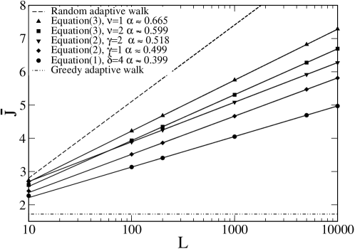
Figure 2: Average number ${\bar{J}}$ of adaptive steps as a function of sequence length $L$ for various fitness distributions when the fitnesses are uncorrelated. The points show the data obtained using numerical simulations and the lines are the best fit to the function ${\bar{J}}=\alpha\ln L+\beta$. The results for greedy walk and random adaptive walk (up to an additive constant) are also shown. The numerical fit for the prefactor $\alpha$ for exponential and uniform fitness distribution matches well with the analytical results given by (46) and (56) respectively.

The results of our numerical simulations for ${\bar{J}}$ shown in Fig. 2 are in agreement with the logarithmic dependence on $L$ but the value of the prefactor does not match with that obtained above (except for $p(f)=e^{-f}$). The prefactor $\alpha$ is expected to interpolate between the two limiting cases of adaptive walks namely greedy walk in which the best mutant is chosen with probability one and random adaptive walk in which all better mutants are chosen with equal probability. The former limit is obtained when $\delta\to 1$ in (1) and the latter when $\nu\to 0$ in (3) (Joyce et al., 2008). Since the average walk length for a greedy walker is a finite constant equal to $e-1\approx 1.718$ for infinitely long sequences (Orr, 2003), the prefactor $\alpha=0$ while $\alpha=1$ for random adaptive walk (see Appendix A). In the following sections, we find that $\alpha=1/2$ for exponentially distributed fitness and $2/3$ for the uniform case which are consistent with the results in Fig. 2 and the analytical results of Neidhart and Krug (2011) which are obtained using a simpler version of the adaptive walk model considered here.

Fitness distribution at the first step for general distributions: If the whole population is assumed to have an initial fitness $f_{0}$, using $P_{0}(f)=\delta(f-f_{0})$ in (7) we have

$$P_{1}(f)=\frac{(f-f_{0})p(f)(1-q^{L}(f_{0}))}{\int_{l}^{u}dg~{}gp(g)}~{}\propto(f-f_{0})p(f)$$ (34)

The above fitness distribution at the first step is nonmonotonic for all fitness distributions in (1)-(3) except for truncated distributions with $\nu\leq 1$. The implications of this result are examined in DISCUSSION.

Entire walk with exponentially distributed fitness: For $p(f)=e^{-f}$, from (11) we obtain

$${\tilde{P}}^{{}^{\prime\prime}}_{J+1}(f)=(1-q^{L}(f)){\tilde{P}}_{J}(f)~{},~{}J\geq 1$$ (35)

where $q(f)=1-e^{-f}$. Due to (12) and (13), the boundary conditions are $P_{J}(0)=0$ and $P_{J}^{\prime}(0)=\delta_{J,1}$.

We define a generating function $G(x,f)=\sum_{J=1}^{\infty}{\tilde{P}}_{J}(f)x^{J}~{},~{}x<1$ which obeys the following second order ordinary differential equation:

$$G^{{}^{\prime\prime}}(x,f)=x(1-q^{L}(f))G(x,f)$$ (36)

To arrive at the above equation, we have used that ${\tilde{P}}_{1}(f)=f$ which is obtained on using the initial condition in (7). The generating function $G(x,f)$ obeys a Schrödinger equation for the wave function of a particle in a one-dimensional potential $V(f)\sim 1-q^{L}(f)$ and energy zero (Mathews and Walker, 1970). Since $1-q^{L}(f)\approx 1-e^{-Le^{-f}}$ is close to unity for $f\ll\ln L$ and vanishes for $f\gg\ln L$, the potential $V(f)$ decreases smoothly from one to zero and moves rightwards with increasing $L$. Similar potentials also arise when two materials with different transport properties are joined together and in such systems, an analytical solution is obtained within a step function potential approximation (Blonder et al., 1982; Schaeybroeck and Lazarides, 2009). We follow this approach here and approximate the distribution $1-q^{L}(f)$ by the Heaviside theta function $\Theta({\tilde{f}}-f)$ where ${\tilde{f}}=\ln L$. Within this step distribution approximation, we have

$$G^{{}^{\prime\prime}}(x,f)=\begin{cases}xG(x,f)~{}&,~{}f<{\tilde{f}}\\ 0~{}&,~{}f>{\tilde{f}}\end{cases}$$ (37)

For $f<{\tilde{f}}$, the differential equation (37) has a solution of the form $G_{<}(x,f)=a_{+}e^{\sqrt{x}f}+a_{-}e^{-\sqrt{x}f}$ which reduces to $G_{<}(x,f)=c\sinh(\sqrt{x}f)$ since $G(x,0)=0$ due to $P_{J}(0)=0$. Since the solution for $f<{\tilde{f}}$ can not depend on ${\tilde{f}}$, we appeal to the infinite sequence length limit to fix the proportionality constant $c$. As noted earlier, the distribution $P_{J}|_{L\to\infty}=1$ for all $J\geq 0$ which implies that

$$\int_{0}^{\infty}df~{}e^{-f}G_{<}(x,f)=\frac{x}{1-x}$$ (38)

and therefore

$$G_{<}(x,f)=\sqrt{x}\sinh(\sqrt{x}f)$$ (39)

We check that the boundary condition $P_{J}^{\prime}(0)={\tilde{P}}_{J}^{\prime}(0)=\delta_{J,1}$ which is equivalent to $G^{\prime}(x,0)=x$ is also satisfied by the above solution.

For $f>{\tilde{f}}$, the solution $G_{>}(x,f)=af+b$ where the constants of integration $a,b$ can be fixed by matching the solutions $G_{<}$ and $G_{>}$ and their first derivative at $f={\tilde{f}}$. Thus the constant $a$ and $b$ are determined by the following conditions:

$$G_{<}(x,{\tilde{f}}) = G_{>}(x,{\tilde{f}})=a{\tilde{f}}+b$$ (40)

$$G^{\prime}_{<}(x,f)|_{f=\tilde{f}} = G^{\prime}_{>}(x,f)|_{f=\tilde{f}}=a$$ (41)

A simple algebra shows that

$$G_{>}(x,f)=x\cosh(\sqrt{x}{\tilde{f}})(f-{\tilde{f}})+\sqrt{x}\sinh(\sqrt{x}{\tilde{f}})$$ (42)

Using the above expressions for $G(x,f)$, the fitness distribution $P_{J}(f)$ for the fixed beneficial mutations can be calculated. On expanding (39) and (42) in a power series about $x=0$ and picking the coefficient of $x^{J}$, we have

$$P_{J}(f)=\frac{e^{-f}f^{2J-1}}{(2J-1)!}\times\begin{cases}1&,~{}r\leq 1\\ \frac{(2J-1)r-(2J-2)}{r^{2J-1}}&,~{}r>1\end{cases}$$ (43)

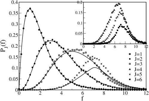
Figure 3: Main: Comparison of the distribution $P_{J}(f)$ for $J=1,2,3,5$ obtained numerically (points) and analytically (lines) given by (43) for exponentially distributed fitness and sequence length $L=1000$. Inset: Numerical data for $P_{J}(f)$ for $J=4,5,6$ to show that the fitness distribution does not shift appreciably beyond ${\bar{J}}\approx 4.6$ as local optimum with average fitness $\approx 7$ is approached.

where $r=f/{\tilde{f}}$. Figure 3 shows our numerical results for $P_{J}(f)$ for the first few adaptive steps. As the walk proceeds, the distribution moves rightwards as expected and its amplitude decreases since the probability $q^{L}(f)$ that the walker can not find a better neighbor approaches unity with increasing $f$. Our analytical result (43) is also shown in Fig. 3 for comparison. For $L=10^{3}$, the step distribution approximation used to find (43) gives $1-q^{L}(f)\approx 1$ for $f<\ln L=6.9$ and zero otherwise. However as the probability $1-q^{L}(f)$ stays close to unity for $f\leq 5$ and decreases gradually to zero when $f\approx 12$, the distribution (43) in the region $5<f<12$ does not match well with the simulation results but outside this crossover region, we see a good quantitative agreement. We also note that the fitness distribution does not move appreciably for $J\geq 4$ and is centred around $f\approx 7$ (see inset of Fig. 3). This is because the average walk length for $L=10^{3}$ is about $4.6$ steps (refer Fig. 2) and as the local optimum is approached, the fitness distribution of fixed beneficial mutation remains centred close to the typical fitness of the local optimum given by (26) which is $\ln L\approx 6.9$. This also explains the initial linear rise in the average fitness followed by a slower increase in Fig. 1.

We next calculate the walk length distribution $Q_{J}$ defined by (17). Since $q^{L}(f)=\Theta(f-{\tilde{f}})$ within the step distribution approximation discussed above, (17) reduces to

$$Q_{J}=\int_{\tilde{f}}^{\infty}df~{}P_{J}(f)$$ (44)

On integrating $P_{J}(f)$ given in (43), we get

$$Q_{J}=e^{-\ln L}\left[\frac{(\ln L)^{2J-2}}{(2J-2)!}+\frac{(\ln L)^{2J-1}}{(2J-1)!}\right]~{},~{}J>0$$ (45)

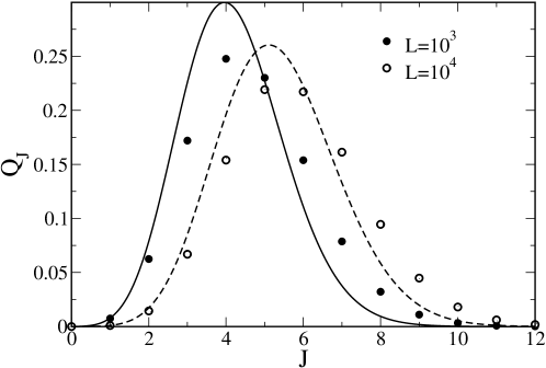
Figure 4: Walk length distribution $Q_{J}$ for $p(f)=e^{-f}$ comparing numerical (points) and analytical result (lines) given by (45).

This expression is compared with numerical results in Fig. 4 and shows a reasonable agreement. The average number of adaptive steps calculated using (45) is given by

$${\bar{J}}=\sum_{J=1}^{\infty}JQ_{J}\approx\frac{1}{2}\ln L$$ (46)

which is in good agreement with the simulation result in Fig. 2. The width of the distribution $Q_{J}$ measured using the variance $\sigma^{2}=\bar{{J^{2}}}-{\bar{J}}^{2}\approx\ln L/4$ also increases with $L$.

Entire walk with uniformly distributed fitness: For $p(f)=1$, since $P_{J}(f)={\tilde{P}}_{J}(f)$, the differential equation (11) reduces to

$$P^{{}^{\prime\prime}}_{J+1}(f)=\frac{1-f^{L}}{\int_{f}^{1}dg~{}(g-f)}~{}P_{J}(f)=\frac{2(1-f^{L})}{(1-f)^{2}}P_{J}(f)~{},~{}J\geq 1$$ (47)

with boundary conditions $P_{J}(0)=0$ and $P_{J}^{\prime}(0)=2\delta_{J,1}$. As before, we define a generating function $G(x,f)=\sum_{J=2}^{\infty}x^{J-2}P_{J}(f)$ which obeys the following second order ordinary differential equation:

$$G^{{}^{\prime\prime}}(x,f)=\frac{2(1-f^{L})}{(1-f)^{2}}~{}(xG(x,f)+2f)$$ (48)

where we have used that $P_{1}(f)=2f$. We treat this case also within the step distribution approximation discussed earlier. Since the probability $1-f^{L}\approx 1-e^{-L(1-f)}$, we approximate it by a step function $\Theta({\tilde{f}}-f)$ where ${\tilde{f}}=(L-1)/L$. For $f<{\tilde{f}}$, we obtain an inhomogeneous second order ordinary differential equation with variable coefficients:

$$G_{<}^{{}^{\prime\prime}}(x,f) = \frac{2x}{(1-f)^{2}}G_{<}(x,f)+\frac{4f}{(1-f)^{2}}$$ (49)

This equation can be solved by standard methods (as detailed in Appendix C) to yield

$$G_{<}(x,f)=a_{+}(1-f)^{\alpha_{+}}+a_{-}(1-f)^{\alpha_{-}}+u_{+}(f)(1-f)^{\alpha_{+}}+u_{-}(f)(1-f)^{\alpha_{-}}$$ (50)

where the exponents

$$\alpha_{\pm}=\frac{1\pm\sqrt{1+8x}}{2}$$ (51)

The first two terms on the right hand side give the solution of the homogeneous equation and the last two terms are the particular integral involving the variational parameters $u_{\pm}(f)$ given in Appendix C. The constants of integration $a_{\pm}$ can be obtained using the boundary conditions $G(x,0)=0$ and $\int_{0}^{1}df~{}G_{<}(x,f)=(1-x)^{-1}$. After some straightforward algebra, we find that

$$G_{<}(x,f)=\frac{-2}{x}\left[\frac{(1-f)^{\alpha_{+}}-(1-f)^{\alpha_{-}}}{\alpha_{+}-\alpha_{-}}+f\right]$$ (52)

We verify that the condition $P_{J}^{\prime}(0)=0$ for $J>1$ which amounts to $G^{\prime}(x,0)=0$ is also satisfied. For $f>{\tilde{f}}$, as $G^{{}^{\prime\prime}}_{>}(x,f)=0$, the solution $G_{>}(x,f)=af+b$ where $a,b$ can be determined using (40) and (41) to give

$$G_{>}(x,f) = \frac{-2}{x}\left[\frac{\alpha_{-}(1-{\tilde{f}})^{\alpha_{-}-1}-\alpha_{+}(1-{\tilde{f}})^{\alpha_{+}-1}}{\alpha_{+}-\alpha_{-}}+1\right]f$$ (53)

$$- \frac{2}{x}\left[\frac{(1-{\tilde{f}})^{\alpha_{+}}-(1-{\tilde{f}})^{\alpha_{-}}-\alpha_{-}{\tilde{f}}(1-{\tilde{f}})^{\alpha_{-}-1}+\alpha_{+}{\tilde{f}}(1-{\tilde{f}})^{\alpha_{+}-1}}{\alpha_{+}-\alpha_{-}}\right]$$

Explicit expressions for $P_{J}(f)$ for first few adaptive steps are given in Appendix C and a comparison between the analytical and the simulation results is shown in Fig. 5.

To find the walk length distribution $Q_{J}=\int_{{\tilde{f}}}^{1}df~{}P_{J}(f)$, we define

$$H(x) = \sum_{J=1}^{\infty}x^{J}Q_{J}=xQ_{1}+x^{2}\int_{\tilde{f}}^{1}df~{}G_{>}(x,f)$$ (54)

$$= \frac{x(1-{\tilde{f}})}{\alpha_{-}-\alpha_{+}}\left[(2-\alpha_{+})(1-{\tilde{f}})^{\alpha_{+}}-(2-\alpha_{-})(1-{\tilde{f}})^{\alpha_{-}}\right]$$ (55)

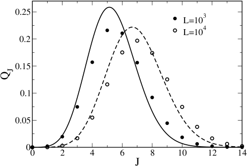
Figure 6: Walk length distribution $Q_{J}$ for uniformly distributed fitnesses comparing simulation (points) and analytical result (lines) in (102).

As an explicit expression for $Q_{J}$ is rather unwieldy, its derivation and the expression itself are given in Appendix C and a comparison with the simulations is shown in Fig. 6. The average number of steps is given by

$${\bar{J}}=\frac{dH(x)}{dx}\bigg{|}_{x=1}=\frac{-6\ln(1-{\tilde{f}})}{9}$$ (56)

which shows that for large $L$, the number of adaptive steps grows as $(2/3)\ln L$ in agreement with the numerical results shown in Fig. 2. The higher moments can also be found straightforwardly and we find that the variance ${\bar{J^{2}}}-{\bar{J}}^{2}\approx(10/27)\ln L$ and the skewness of the distribution decays slowly as $(\ln L)^{-1/2}$.

Effect of correlations on the number of adaptive steps: We now turn to a discussion of adaptive walk properties when the fitnesses are correlated and given by a block model. We compute the average number ${\bar{J}}_{B}(L)$ of adaptive steps given by $\sum_{J=1}^{\infty}JQ_{J}(L,B)$ where $Q_{J}(L,B)$ is the probability that exactly $J$ adaptive mutations occur when a sequence of length $L$ is divided in $B$ blocks.

Consider the distribution ${\cal Q}(m_{1},...,m_{B})$ which gives the joint probability that the $i$th block of length $L_{B}$ in a sequence of length $L$ carries $m_{i}$ adaptive mutations where $i=1,...,B$. An important property of the block model is that this joint distribution factorises, that is (Perelson and Macken, 1995)

$${\cal Q}(m_{1},...,m_{B})=\prod_{b=1}^{B}Q_{m_{b}}(L_{B},1)$$ (57)

where $Q_{J}(L_{B},1)\equiv Q_{J}(L_{B})$ is the walk length probability when the fitnesses are uncorrelated and the sequence length is $L_{B}$. The above equation expresses the fact that the block fitnesses evolve independently. As only one mutation occurs in the sequence at any step so that all but one block sequence remains unchanged and since the block fitnesses are i.i.d. random variables, (57) holds.

Since the distribution $Q_{J}(L,B)$ is given by

$$Q_{J}(L,B)=\sum_{m_{1},...,m_{B}=0}^{J}{\cal Q}(m_{1},...,m_{B})\delta(m_{1}+...+m_{B}-J)$$ (58)

it follows that

$${\bar{J}}_{B}(L) = \sum_{J=1}^{\infty}J\sum_{m_{B}=0}^{J}Q_{m_{B}}(L_{B})\sum_{m_{1},...,m_{B-1}=0}^{J-m_{B}}\prod_{b=1}^{B-1}Q_{m_{b}}(L_{B})\delta(\sum_{b=1}^{B-1}m_{b}-(J-m_{B}))$$ (59)

$$= \sum_{J=1}^{\infty}J\sum_{m_{B}=0}^{J}Q_{m_{B}}(L_{B})Q_{J-m_{B}}(L-L_{B},B-1)$$

$$= \sum_{m=0}^{\infty}Q_{m}(L-L_{B},B-1)\sum_{n=0}^{\infty}(n+m)Q_{n}(L_{B})$$

$$= {\bar{J}}(L_{B})+\sum_{m=1}^{\infty}mQ_{m}(L-L_{B},B-1)$$

$$= {\bar{J}}(L_{B})+{\bar{J}}_{B-1}(L-L_{B})$$

$$= B{\bar{J}}(L_{B})$$

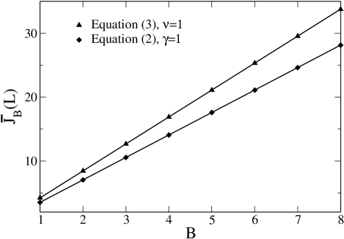
Figure 7: Average number ${\bar{J}}_{B}$ of adaptive steps as a function of block number $B$ for fixed $L/B=100$. The numerical data is in excellent agreement with (59) shown by solid line.

where we have used that $\sum_{J=0}^{\infty}Q_{J}(L,B)=1$ and ${\bar{J}}$ is the average number of steps in the adaptive walk for uncorrelated fitnesses. Figure 7 shows the results of our numerical simulations for average walk length when the block length $L_{B}=L/B$ is kept fixed and the block fitnesses are exponentially and uniformly distributed. For fixed $L_{B}$, (59) predicts that ${\bar{J}}_{B}$ increases linearly with $B$ which is in excellent agreement with the numerical data.

For large $L$, due to (33) we have

$${\bar{J}}_{B}(L)\approx\alpha B\ln(L/B)$$ (60)

For small $B$, a linear rise in the average number of steps with the number of blocks has been seen numerically for exponential-like distributions and it was inferred that the mean walk length is independent of underlying fitness distributions (Orr, 2006). However as discussed in the previous sections, the average number ${\bar{J}}$ depends on the fitness distribution $p(f)$ and therefore the average ${\bar{J}}_{B}$ is also nonuniversal.

DISCUSSION

In the last few years, several analytical results have been obtained for the mutational landscape model (Gillespie, 1991). However many of these results deal with the first step in the adaptation process (Orr, 2002, 2006; Joyce et al., 2008) and an extension of the theory to full adaptive walk is necessary. Previous studies also assume that the process of adaptation starts from a highly fit sequence which is not applicable to situations in which the population is subjected to high stress and hence has a very low initial fitness (MacLean and Buckling, 2009; McDonald et al., 2010). In this article, we have obtained results for the entire adaptive walk starting from a low initial fitness but as discussed below, we expect some of these results to hold for moderately high initial fitness also.

Walk length distribution and average walk length: In previous works, the walk length distribution for the greedy walk and the random adaptive walk have been studied and found to be universal in that they are independent of the underlying fitness distribution $p(f)$. The origin of this universality property is clear in the light of the results of Joyce et al. (2008) who pointed out that these two models can be obtained as a limit of (4) which defines the mutational landscape model. For the random adaptive walk, the distribution $Q_{J}$ for infinitely long sequence vanishes (see (63)) and the average walk length diverges with sequence length. In contrast, for greedy walk, the walk length distribution in the $L\to\infty$ limit decreases exponentially fast with $J$ for the greedy walk as a result of which the average number of steps turns out to be a constant (Orr, 2003; Rosenberg, 2005).

In this article, we have calculated the walk length distribution for exponentially and uniformly distributed fitnesses and found the average walk length for general fitness distributions. An important conclusion of our study is that the average number of adaptive steps increases logarithmically with the sequence length with a prefactor smaller than unity if the walk starts from zero fitness. Our simulations (not shown) also indicate that if the initial rank is of order $L$, the average number of steps increases logarithmically with the rank and with the same proportionality constant as that for the zero initial fitness case. Thus for a wild type sequence with initial rank (or $L$) of the order $100$, the number of substitutions are expected to be less than $5$. Although short adaptive walks have been observed in experiments (Rokyta et al., 2009; Schoustra et al., 2009), more detailed experimental studies testing the logarithmic dependence would be desirable. Although a test of the $L$-dependence of the average walk length may not be experimentally viable, it should be possible to study the average walk length as a function of the initial rank.

Besides the sequence length, the number of steps to a local optimum depend on the underlying fitness distribution and the fitness correlations also. If the fitnesses are uncorrelated, as the numerical data in Fig. 2 shows, the prefactor $\alpha$ in (33) depends on the shape of the fitness distribution and therefore a rather detailed knowledge of the full fitness distribution (how fast it decays) is required to test this which is presently unavailable. However one can discern a trend in the value of $\alpha$: it decreases as the fitness distribution broadens. This suggests that systems with fitness distribution in the Gumbel class (Imhof and Schlotterer, 2001; Sanjuán et al., 2004; Rokyta et al., 2005; Kassen and Bataillon, 2006; MacLean and Buckling, 2009) will register shorter walks than those in the Weibull domain (Rokyta et al., 2008). As shown here in the block model of correlated fitnesses, the average number of adaptive steps increases as the number of blocks (and hence fitness correlations) increase. This is in accordance with the expectation that on a smooth correlated fitness landscape, as the local optima are less common (Perelson and Macken, 1995), there is a less chance to get trapped and therefore uphill walk can last longer (Weinberger, 1991; Kauffman, 1993; Orr, 2006).

Distribution of fixed beneficial mutations during the walk: The fitness distribution $P_{J}(f)$ has not been studied in previous theoretical studies of adaptive walks in the SSWM limit and here we have computed this fitness distribution analytically using the recursion relation (7). The fitness distribution at the first step given by (34) can give a qualitative idea about the shape of $p(f)$. For most fitness distributions, $P_{1}(f)$ is expected to be nonmonotonic but for bounded distributions which diverge at the upper limit or the uniform distribution, $P_{1}(f)$ increases monotonically towards the upper bound. An inspection of the experimental data of Rokyta et al. (2005) shows the fitness distribution at the first step to be nonmonotonic which is consistent with their assumption of exponentially decreasing distribution of beneficial effects. It would be interesting to check if the distribution $P_{1}(f)$ in Rokyta et al. (2008) is monotonic as the data in this study is consistent with a uniformly distributed fitness. The above behavior of $P_{1}(f)$ is expected to be robust in the presence of correlations as at the first step in evolution, the population has not sensed the correlations in the fitness landscape (Orr, 2006).

For the fitness distribution for the entire walk, we presented an analysis for two distributions namely exponential and uniform which are consistent with the available experimental data. The distribution $P_{J}(f)$ is obtained within a step distribution approximation which captures the shape of the fitness distribution correctly for the first few steps and leads to an accurate estimate of the number of average steps. Our approximation consists of replacing the probability $1-q^{L}(f)$ by a step function $\Theta({\tilde{f}}-f)$ where ${\tilde{f}}$ is given by (28) for exponentially and (29) for uniformly distributed fitnesses. For $f\ll{\tilde{f}}$ and $f\gg{\tilde{f}}$, our approximate solution matches the simulation results well for any $J$. With increasing $J$, the distribution $P_{J}(f)$ shifts towards higher fitnesses and peaks about ${\tilde{f}}$ for larger $J$’s. As explained earlier, the fitness ${\tilde{f}}$ is reached when $J$ is close to ${\bar{J}}\propto\ln L$ and therefore we expect our approximation to work well for $J\ll\ln L$.

When the underlying fitness distribution is exponential, we find that the fitness distribution of the fixed beneficial mutation also has an exponential tail (see (43)). The robustness of this result i.e. whether any fitness distribution in the Gumbel class exhibits exponential tail for $P_{J}(f)$ is however not clear. For uniformly distributed fitnesses, as the width of the distribution $1-q^{L}(f)$ decreases with increasing $L$, the step distribution approximation works better in this case than in the exponential case where the width is a constant (compare Figs. 4 and 6). The properties of multiple steps in an adaptive walk have been measured in some recent experiments (Rokyta et al., 2009; Schoustra et al., 2009) and a detailed analysis of the experimental results would be very welcome. On the theoretical front, an extension of the results described above to distributions other than uniform and exponential would be desirable. We have recently made some progress in this direction and the results will appear elsewhere.

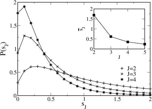
Figure 8: Distribution $P(s_{J})$ of selection coefficient $s_{J}$ for $L=1000$ and $p(f)=e^{-f}$. The inset shows the decay in average selection coefficient ${\bar{s}}_{J}$ as a function of $J$. The points are joined by line to guide the eye.

Another interesting question concerns the distribution $P(s_{J})$ of the selection coefficient $s_{J}=(f_{J}-f_{J-1})/f_{J-1}$ at the $J$th step in the adaptive walk. As we start with zero fitness, the selection coefficient is defined for $J\geq 2$. Our preliminary numerical results for $P(s_{J})$ are shown in Fig. 8 for the first few steps in the walk and we observe that the typical selection coefficient decreases as the walk proceeds. This behavior matches qualitatively with the experimental results of Schoustra et al. (2009). A theoretical analysis of the distribution $P(s_{J})$ requires the joint distribution of the fitness at step $J-1$ and $J$ and we hope to address this question in a future work.

Acknowledgement: K.J. thanks J. R. David for helpful suggestions, J. Krug for comments on an earlier version of the manuscript and useful correspondence and KITP, Santa Barbara for hospitality and support under the NSF Grant No. PHY05-51164. The authors also thank L. Wahl for suggestions to improve the manuscript.

APPENDIX A: RANDOM ADAPTIVE WALK

In this Appendix, we briefly review the known results for random adaptive walk in which all better mutants are chosen with equal probability (Macken and Perelson, 1989; Flyvbjerg and Lautrup, 1992; Kauffman, 1993). The probability distribution $P_{J}(f)$ obeys the following recursion relation (Flyvbjerg and Lautrup, 1992):

$$P_{J+1}(f)=\int_{l}^{f}dh~{}\frac{p(f)}{\int_{h}^{u}dg~{}p(g)}~{}\left[1-q^{L}(h)\right]P_{J}(h)$$ (61)

where $q(f)=\int_{l}^{f}dg~{}p(g)$. A change of variable from the fitness $f$ to the cumulative probability $q(f)$ gives

$${P}_{J+1}(q)=\int_{0}^{q}dq^{\prime}\frac{1-q^{\prime L}}{1-q^{\prime}}~{}{P}_{J}(q^{\prime})$$ (62)

Since the walk length distribution for the random adaptive walk also obeys (17), we have

$$Q_{J}=\int_{l}^{u}dh~{}q^{L}(h)P_{J}(h)=\int_{l}^{u}dq~{}q^{L}{P}_{J}(q)$$ (63)

which shows that $Q_{J}$ is a universal distribution in that it is independent of the underlying fitness distribution $p(f)$. Note that for infinitely long sequences, the probability $Q_{J}=0$ as in the mutational landscape model. Differentiating (62) with respect to $q$ immediately gives

$$\frac{d{P}_{J+1}(q)}{dq}=\frac{1-q^{L}}{1-q}~{}{P}_{J}(q)=\sum_{n=0}^{L}q^{n}~{}{P}_{J}(q)$$ (64)

The generating function $G(x,q)=\sum_{J=1}^{\infty}x^{J}{P}_{J}(q)$ then obeys the following first order differential equation:

$$G^{\prime}(x,q)-x{P}_{1}^{\prime}(q)=x\frac{1-q^{L}}{1-q}G(x,q)$$ (65)

For the initial condition $P_{0}(f)=\delta(f)$, we have $P_{1}(q)=1$ and due to (62), the distribution ${P}_{J}(0)=0$. Solving the above differential equation using these boundary conditions gives $G(x,q)=xe^{xH_{L}(q)}$ where $H_{L}(q)=\sum_{k=1}^{L}q^{k}/k$ and hence the distribution ${P}_{J}(q)$ is given by (Flyvbjerg and Lautrup, 1992)

$${P}_{J}(q)=\frac{H^{J-1}_{L}(q)}{(J-1)!}$$ (66)

Since the product $q^{L}{P}_{J}(q)$ in (63) peaks around $q=1$, using $H_{L}(q)\approx\ln L$ for $q$ close to unity for finite but long sequences and performing the integral in (63), we get

$$Q_{J}\approx e^{-\bar{J}}\frac{{\bar{J}}^{J-1}}{(J-1)!}$$ (67)

where ${\bar{J}}=\ln L$. Thus the walk length distribution is a Poisson distribution (in $J$) with mean ${\bar{J}}=\ln L$ (Flyvbjerg and Lautrup, 1992).

APPENDIX B: SIMULATION PROCEDURE

For short sequences of length $L\leq 10$ and uncorrelated fitnesses, a randomly chosen sequence was assigned a fitness equal to zero. Then the rest of the fitness landscape comprising of $2^{L}-1$ fitnesses was generated by drawing random variables independently from a common distribution $p(f)$. The transition probability from the initial sequence to each of the better sequences among the $L$ nearest neighbors was calculated according to (4) and the fixed sequence at the first step in the adaptive walk was chosen. Then the transition probability from the chosen mutant sequence to its better neighbors was calculated and this process was repeated until a fitter sequence was not available.

To simulate sequences with length $L\gtrsim 10^{2}$, we followed an approximate procedure outlined in Orr (2002) as the total number of sequences $2^{L}$ is prohibitively large for long sequences. Starting with zero fitness, $L$ i.i.d. random variables were generated and a higher fitness $f$ was chosen according to the transition probability (4). During the next step in the process, $L$ new i.i.d. random variables were generated and the transition probability from $f$ to a better fitness was calculated. These steps were repeated until the new set of random fitnesses does not exceed the currently fixed fitness. The block model was simulated to generate weakly correlated fitnesses by assigning independent fitnesses to each block sequence. In all the simulations, the data was collected using $10^{6}$ independent realisations of the fitness landscape.

APPENDIX C: DERIVATIONS FOR UNIFORMLY DISTRIBUTED FITNESS

Solution of differential equation 49: The generating function $G_{<}(x,f)$ obeys the following inhomogeneous second order differential equation:

$$G^{{}^{\prime\prime}}(x,f)-\frac{2x}{(1-f)^{2}}G(x,f)=\frac{4f}{(1-f)^{2}}$$ (68)

where we have dropped the subscript for brevity. The general solution of such differential equations is a linear combination of the general solution $G_{H}(x,f)$ of the homogeneous equation obtained by setting the right hand side equal to zero and the particular solution $G_{P}$ of the inhomogeneous equation (Mathews and Walker, 1970). The homogeneous solution is of the form

$$G_{H}(x,f)=a_{+}(1-f)^{\alpha_{+}}+a_{-}(1-f)^{\alpha_{-}}$$ (69)

where $\alpha_{\pm}$ are the solutions of the quadratic equation $\alpha^{2}-\alpha-2x=0$ and given by (51). The particular solution is found using the method of variation of parameters and is of the form $G_{P}(x,f)=u_{+}(x)(1-f)^{\alpha_{+}}+u_{-}(x)(1-f)^{\alpha_{-}}$ where the functions $u_{\pm}(f)$ obey the following first order differential equations (Mathews and Walker, 1970):

$$u^{\prime}_{+}(f)(1-f)^{\alpha_{+}}+u^{\prime}_{-}(f)(1-f)^{\alpha_{-}} = 0$$ (70)

$$\alpha_{+}u^{\prime}_{+}(f)(1-f)^{\alpha_{+}-1}+\alpha_{-}u^{\prime}_{-}(f)(1-f)^{\alpha_{-}-1} = \frac{4f}{(1-f)^{2}}$$ (71)

On solving the above equations, we obtain

$$G_{P}(x,f)=\frac{4}{\alpha_{+}\alpha_{-}}-\frac{4(1-f)}{(1-\alpha_{+})(1-\alpha_{-})}=\frac{-2f}{x}$$ (72)

Finally using the boundary conditions in the general solution $G_{<}(x,f)=G_{P}(x,f)+G_{H}(x,f)$, the desired result (52) is obtained.

Distribution of fixed beneficial mutations: The fitness distribution found using (52) and (53) is given below for the first few adaptive steps:

$$P_{1}(f) = 2f~{}~{}~{}~{},~{}f\leq 1$$ (73)

$$P_{2}(f) = \left\{\begin{array}[]{ll}-8f+4(f-2)\ln(1-f)&,~{}f\leq{\tilde{f}}\\ \frac{4{\tilde{f}}(f+{\tilde{f}}-2)}{1-{\tilde{f}}}+4(f-2)\ln(1-{\tilde{f}})&~{},~{}f>{\tilde{f}}\end{array}\right.$$ (76)

$$P_{3}(f) = 4\left\{\begin{array}[]{ll}12f+\ln(1-f)(12-6f+f\ln(1-f))&,~{}f\leq{\tilde{f}}\\ \frac{1}{1-{\tilde{f}}}\left[6{\tilde{f}}(2-f-{\tilde{f}})+2(6-(6-{\tilde{f}}){\tilde{f}}-f(3-2{\tilde{f}}))\ln(1-{\tilde{f}})\right.\\ +\left.f(1-{\tilde{f}})\ln^{2}(1-{\tilde{f}})\right]&,~{}f>{\tilde{f}}\end{array}\right.$$ (80)

$$P_{4}(f) = \frac{-8}{3}\left\{\begin{array}[]{ll}120f+60(2-f)\ln(1-f)+12f\ln^{2}(1-f)+(2-f)\ln^{3}(1-f)~{},~{}f\leq{\tilde{f}}\\ \frac{1}{(1-{\tilde{f}})}\left[60{\tilde{f}}(2-f-{\tilde{f}})-12(f(5-3{\tilde{f}})-2(5-(5-{\tilde{f}}){\tilde{f}}))\ln(1-{\tilde{f}})\right.\\ +\left.3(f(2-3{\tilde{f}})+(2-{\tilde{f}}){\tilde{f}})\ln^{2}(1-{\tilde{f}})+(2-f)(1-{\tilde{f}})\ln^{3}(1-{\tilde{f}})\right]~{},~{}f>{\tilde{f}}\end{array}\right.$$ (84)

Walk length distribution: On matching powers of $x^{J}$ on both sides in (55), we get

$$Q_{1} = e^{-2\ell}(-1+2e^{\ell})$$ (85)

$$Q_{2} = 2e^{-2\ell}(3+\ell+(-3+2\ell)e^{\ell})$$ (86)

$$Q_{3} = e^{-2\ell}\left[-2(18+8\ell+\ell^{2})+4e^{\ell}(9-5\ell+\ell^{2})\right]$$ (87)

$$Q_{4} = \frac{4e^{-2\ell}}{3}\left[180+84\ell+15\ell^{2}+\ell^{3}+e^{\ell}(-180+96\ell-21\ell^{2}+2\ell^{3})\right]$$ (88)

where $\ell=\ln L$. A general solution of $Q_{J}$ by this method does not seem possible but an approximate analytic expression for $Q_{J}$ can be obtained as explained below.

From the definition of the generating function $H(x)$ in (55), it follows that

$$Q_{J}=\frac{1}{J!}\frac{d^{J}H(x)}{dx^{J}}\bigg{|}_{x=0}$$ (89)

By the residue theorem for complex variables, we have (Mathews and Walker, 1970)

$$\frac{1}{2\pi i}\int_{C}dz~{}f(z)=\frac{1}{n!}\frac{d^{n}}{dz^{n}}\left((z-z_{0})^{n+1}f(z)\right)\bigg{|}_{z=z_{0}}$$ (90)

where $z_{0}$ is a pole of order $n+1$ of the function $f(z)$ and the contour $C$ encloses the singularities of $f(z)$. From (89) and (90), we can write

$$Q_{J}=\frac{1}{2\pi i}\int_{C}dz~{}\frac{H(z)}{z^{J+1}}=\frac{1}{2\pi i}\int_{C}dz~{}e^{K(z)}$$ (91)

where $K(z)=\ln H(z)-(J+1)\ln z$. We solve this integral by the method of steepest descent which for large $J$ gives (Mathews and Walker, 1970)

$$Q_{J}\approx\sqrt{\frac{1}{2\pi K^{\prime\prime}(z_{s})}}e^{K(z_{s})}=\sqrt{\frac{1}{2\pi K^{\prime\prime}(z_{s})}}\frac{H(z_{s})}{z_{s}^{J+1}}$$ (92)

where prime refers to derivative with respect to $z$. In the above equation, $z_{s}$ is a solution of the equation

$$\frac{H^{\prime}(z_{s})}{H(z_{s})}=\frac{J}{z_{s}}$$ (93)

and

$$K^{\prime\prime}(z_{s}) = \left(\frac{H^{\prime}(z)}{H(z)}\right)^{\prime}\bigg{|}_{z=z_{s}}+\frac{J}{z_{s}^{2}}$$ (94)

$$= \left(\frac{H^{\prime}(z)}{H(z)}\right)^{\prime}\bigg{|}_{z=z_{s}}+\frac{1}{z_{s}}\frac{H^{\prime}(z_{s})}{H(z_{s})}$$ (95)

where prime denotes a derivative with respect to $z$. Since $\alpha_{+}>0$, neglecting the exponentially small term in $(1-{\tilde{f}})^{\alpha_{+}}$ in (55), we get

$$H(z)\approx\frac{e^{-3\ell/2}e^{\ell y/2}(3+y)(y^{2}-1)}{16y}$$ (96)

where $y=\sqrt{1+8z}$. Differentiating $H(z)$ once with respect to $z$ gives

$$\frac{H^{\prime}(z)}{H(z)}\approx\frac{8(y+3)+4(2y+3)(y^{2}-1)+2y(y+3)(y^{2}-1)\ell}{y^{2}(y^{2}-1)(y+3)}$$ (97)

Using the above expression in (93) for large $y$, we get $y_{s}\approx 4J/\ell$ and therefore

$$z_{s}\approx\frac{2J^{2}}{\ell^{2}}$$ (98)

On differentiating (97) once, we have

$$\left(\frac{H^{\prime}(z)}{H(z)}\right)^{\prime}\approx\frac{4}{y}\left[\frac{4}{3(y+3)^{2}}+\frac{4}{(1+y)^{2}}-\frac{4+6\ell}{3y^{2}}+\frac{8}{y^{3}}-\frac{4}{(1-y)^{2}}\right]$$ (99)

Using (97) and (99) in (95), we obtain

$$K^{\prime\prime}(z_{s}) \approx \frac{8\left[-36+6y_{s}(y_{s}^{2}-3)+y_{s}(y_{s}+3)^{2}(1+y_{s})^{2}\ell\right]}{y_{s}^{4}(y_{s}+3)^{2}(y_{s}^{2}-1)}$$ (100)

$$\approx \frac{8\ell}{y_{s}^{3}}=\frac{a^{4}}{8J^{3}}$$ (101)

Thus we have

$$Q_{J}\approx\frac{2J^{3/2}}{\sqrt{\pi}\ell^{2}}\times\frac{2-\alpha_{-}(z_{s})}{\alpha_{+}(z_{s})-\alpha_{-}(z_{s})}\times\frac{(1-{\tilde{f}})^{1+\alpha_{-}(z_{s})}}{z_{s}^{J}}$$ (102)

where $\alpha_{\pm}$ is given by (51).

Figure 5: Comparison of the distribution $P_{J}(f)$ for $J=1,2,3,4$ obtained numerically (points) and analytically (lines) given by (73)-(84) for uniformly distributed fitness and sequence length $L=100$. The distribution for $f\leq{\tilde{f}}$ is shown in the main plot and for $f>{\tilde{f}}$ in the inset.

References

- Blonder et al. (1982) Blonder, G. E., M. Tinkham, and T. M. Klapwijk, 1982 Transition from metallic to tunneling regimes in superconducting microconstrictions: Excess current, charge imbalance, and supercurrent conversion. Phys. Rev. B 25: 4515.
- Bull and Otto (2005) Bull, J. J. and S. P. Otto, 2005 The first steps in adaptive evolution. Nat. Genet. 37: 342–343.
- Carneiro and Hartl (2010) Carneiro, C. and D. Hartl, 2010 Adaptive landscapes and protein evolution. Proc. Natl. Acad. Sci. USA 107: 1747–1751.
- David and Nagaraja (2003) David, H. and H. Nagaraja, 2003 Order Statistics. Wiley, New York.
- Eyre-Walker and Keightley (2007) Eyre-Walker, A. and P. Keightley, 2007 The distribution of fitness effects of new mutations. Nat. Rev. Genet. 8: 610.
- Flyvbjerg and Lautrup (1992) Flyvbjerg, H. and B. Lautrup, 1992 Evolution in a rugged fitness landscape. Phys. Rev. A 46: 6714–6723.
- Gillespie (1983) Gillespie, J. H., 1983 A simple stochastic gene substitution process. Theor. Popul. Biol. 23: 202–215.
- Gillespie (1991) Gillespie, J. H., 1991 The Causes of Molecular Evolution. Oxford University Press, Oxford.
- Imhof and Schlotterer (2001) Imhof, M. and C. Schlotterer, 2001 Fitness effects of advantageous mutations in evolving Escherichia coli populations. Proc. Natl. Acad. Sci. USA 98: 1113–1117.
- Jain (2011) Jain, K., 2011 Extreme value distributions for weakly correlated fitnesses in block model. J. Stat. Mech.: P04020.
- Jain et al. (2009) Jain, K., A. Dasgupta, and G. Das, 2009 Exact and limit distributions of the largest fitness on correlated fitness landscapes. J. Stat. Mech.: L10001.
- Joyce et al. (2008) Joyce, P., D. R. Rokyta, C. J. Beisel, and H. A. Orr, 2008 A general extreme value theory model for the adaptation of DNA sequences under strong selection and weak mutation. Genetics 180: 1627–1643.
- Kassen and Bataillon (2006) Kassen, R. and T. Bataillon, 2006 Distribution of fitness effects among beneficial mutations before selection in experimental populations of bacteria. Nat. Genet. 38: 484–488.
- Kauffman (1993) Kauffman, S. A., 1993 The Origins of Order. Oxford University Press, New York.
- Macken and Perelson (1989) Macken, C. A. and A. S. Perelson, 1989 Protein evolution on rugged landscapes. Proc. Natl. Acad. Sci. USA 86: 6191–6195.
- MacLean and Buckling (2009) MacLean, R. and A. Buckling, 2009 The distribution of fitness effects of beneficial mutations in Pseudomonas aeruginosa. PLoS Genetics 5: e1000406.
- Mathews and Walker (1970) Mathews, J. and R. L. Walker, 1970 Mathematical methods of physics. Pearson Education Limited.
- McDonald et al. (2010) McDonald, M., T. F. Cooper, H. J. E. Beaumont, and P. B. Rainey, 2010 The distribution of fitness effects of new beneficial mutations in Pseudomonas fluorescens. Biol. Lett. 7: 98–100.
- Miller et al. (2011) Miller, C. R., P. Joyce, and H. Wichman, 2011 Mutational effects and population dynamics during viral adaptation challenge current models. Genetics 187: 185–202.
- Neidhart and Krug (2011) Neidhart, J. and J. Krug, 2011 Adaptive walks and extreme value theory. arXiv:1105.0592.
- Orr (2003) Orr, H., 2003 A minimum on the mean number of steps taken in adaptive walks. J. theor. Biol. 220: 241–247.
- Orr (2002) Orr, H. A., 2002 The population genetics of adaptation: The adaptation of DNA sequences. Evolution 56: 1317–1330.
- Orr (2006) Orr, H. A., 2006 The population genetics of adaptation on correlated fitness landscapes: The block model. Evolution 60: 1113.
- Perelson and Macken (1995) Perelson, A. and C. Macken, 1995 Protein evolution on partially correlated landscapes. Proc. Natl. Acad. Sci. USA 92: 9657–9661.
- Rokyta et al. (2009) Rokyta, D., Z. Abdo, and H. Wichman, 2009 The genetics of adaptation for eight microvirid bacteriophages. J Mol Evol 69: 229.
- Rokyta et al. (2008) Rokyta, D., C. J. Beisel, P. Joyce, M. T. Ferris, C. L. Burch, and H. Wichman, 2008 Beneficial fitness effects are not exponential for two viruses. J Mol Evol 69: 229.
- Rokyta et al. (2005) Rokyta, D., P. Joyce, S. Caudle, and H. Wichman, 2005 An empirical test of the mutational landscape model of adaptation using a single-stranded DNA virus. Nat. Genet. 37: 441–444.
- Rosenberg (2005) Rosenberg, N., 2005 A sharp minimum on the mean number of steps taken in adaptive walks. J. theor. Biol. 237: 17–22.
- Rozen et al. (2002) Rozen, D., J. de Visser, and P. J. Gerrish, 2002 Fitness effects of fixed beneficial mutations in microbial populations. Curr Biol. 12: 1040–1045.
- Sanjuán et al. (2004) Sanjuán, R., A. Moya, and S. Elena, 2004 The distribution of fitness effects caused by single-nucleotide substitutions in an RNA virus. Proc. Natl. Acad. Sci. USA 101: 8396–8401.
- Schaeybroeck and Lazarides (2009) Schaeybroeck, v. B. and A. Lazarides, 2009 Normal-Superfluid Interface for Polarized Fermion Gases. Phys. Rev. A 79: 053612.
- Schoustra et al. (2009) Schoustra, S., T. Bataillon, D. Gifford, and R. Kassen, 2009 The properties of adaptive walks in evolving populations of fungus. PLoS Biol 7 (11): e1000250.
- Sornette (2000) Sornette, D., 2000 Critical Phenomena in Natural Sciences. Springer, Berlin.
- Weinberger (1991) Weinberger, E. D., 1991 Local properties of Kauffman’s N-k model: a tunably rugged energy landscape. Phys. Rev. A 44: 6399–6413.