Non-Gaussian fluctuations in stochastic models with absorbing barriers

Abstract

The dynamics of a one-dimensional stochastic model is studied in presence of an absorbing boundary. The distribution of fluctuations is analytically characterized within the generalized van Kampen expansion, accounting for higher order corrections beyond the conventional Gaussian approximation. The theory is shown to successfully capture the non Gaussian traits of the sought distribution returning an excellent agreement with the simulations, for all times and arbitrarily close to the absorbing barrier. At large times, a compact analytical solution for the distribution of fluctuations is also obtained, bridging the gap with previous investigations, within the van Kampen picture and without resorting to alternative strategies, as elsewhere hypothesized.

Studying the dynamics of large ensemble of interacting entities is a fascinating field of investigations of broad applied and fundamental interest. Atom and nuclei result for instance in extended systems of mutually interacting discrete elements. Similarly, proteins can be ideally imagined as a coherent sea of microscopic actors that e.g. densely populate the inside of the cells. Social and human communities are also examples of systems that display rather intricate dynamics, microscopically governed by the very complex network of interlaced connections among individuals. Surprisingly, and as follows a widespread observation of cross-disciplinary breath, regular collective modes can spontaneously emerge at the macroscopic level, as resulting from the erratic dynamics of the microscopic discrete constituents McKane and Newman (2005); Dauxois et al. (2009); de Anna et al. (2010); Biancalani et al. (2010).

The time evolution of such inherent stochastic system is generally described in terms of a master equation Gardiner (1985), a differential equation for the probability of observing the scrutinized system in a certain configuration at given time. In practically all cases of interest, solving the master equation proves a task of formidable complexity, and approximated strategies need to be implemented to gain analytical insight into the system being examined. The celebrated van Kampen expansion van Kampen (1992) represents a viable technique to enable one for analytical progress. It is customarily believed that such a method works efficiently well provided the system is defined in a open domain or, conversely, if it evolves sufficiently far from any existing boundaries McKane and Newman (2005). As an emblematic example, when the system has to face an asymptotic extinction, thus evolving towards an attractive absorbing state, the van Kampen perturbative scheme is only assumed appropriate for short times. Recently, and to eventually bypass these supposedly stringent limitations, a different perturbative approach has been pioneered in Di Patti et al. (2011) that suites for large times, when the system is feeling the absorbing barrier. Working within this generalized setting, and operating with reference to a paradigmatic model of systems with an absorbing state, the voter model, a closed expression for the distribution of fluctuations was obtained which agrees with direct simulations. The derivation rests however on speculative grounds, which, despite the a posteriori validation, seem to lack of a solid physical interpretation, fully justified from first principles.

The purposes of this Letter are twofold. On the one side, and with reference to the same version of the voter model as considered in Di Patti et al. (2011), we will analytically demonstrate that by extending the van Kampen expansion to include higher orders corrections Grima (2009), beyond the classical approximation, allows us to accurately reproduce the observed distribution of fluctuations at any time. Non Gaussian traits reflecting the presence of the absorbing barrier are nicely captured by the method, which proves therefore accurate also close to the boundary. Even more interesting, the van Kampen solution is shown to converge at late times to the distribution calculated in Di Patti et al. (2011), this latter being hence explained within a sound and universal descriptive picture.

Let us start by introducing the stochastic discrete voter model. As in the spirit of Di Patti et al. (2011), we consider a system made of $N$ elements in mutual interactions, possibly organized in different species. Label with $X_{1}$ the elements of a specific species and with $X_{0}$ all the other entities. The following chemical equations are proposed to rule the microscopic dynamics:

$$X_{1}+X_{0}\stackrel{{\scriptstyle 1}}{{\longrightarrow}}2X_{0},$$

$$X_{0}+X_{1} \stackrel{{\scriptstyle 1-\nu}}{{\longrightarrow}} 2X_{1},$$

$$X_{1}+X_{1} \stackrel{{\scriptstyle\nu}}{{\longrightarrow}} X_{1}+X_{0}$$

The master equation which stems from the above system reads:

$$\frac{d}{dt}P_{n}(t) = (\epsilon_{n}^{-}-1)[T(n+1|n)P_{n}(t)]$$ (1)

$$+(\epsilon_{n}^{+}-1)[T(n-1|n)P_{n}(t)]$$

where $P_{n}(t)$ is the probability of photographing the system at time $t$ in a configuration with $n$ individuals belonging to the population of $X_{1}$ and $\epsilon_{n}^{\pm}$ are the step operators van Kampen (1992). The transition rates are given by:

$$T(n+1|n) = (1-\nu)\frac{(N-n)}{N}\frac{n}{N}$$

$$T(n-1|n) = \frac{n}{N}\frac{N-n}{N}+\nu\frac{n}{N}\frac{n}{N}$$

where the initial states are the right entries and the final states the left ones. As follows the above, $n=0$ is an absorbing state while $n=N$ corresponds to a reflecting barrier. The van Kampen approach requires imposing:

$$\frac{n}{N}=\phi(t)+\frac{\xi}{\sqrt{N}}$$ (2)

where $1/\sqrt{N}$ plays the role of a small parameter and paves the way to the perturbative expansion hereafter discussed. By inserting the working ansatz (2) into the master equation (1), and hierarchically organizing the resulting terms with respect to their $N$-dependence, one obtains at the first order the mean-field deterministic equation for the continuum concentration $\phi(\tau)$ ($\tau$ being the rescaled time $t/N$), namely $d\phi/d\tau=-\nu\phi$, whose solution reads $\phi(\tau)=\phi_{0}\exp(-\nu\tau)$. Higher order contributions results in a generalized Fokker-Planck equation for the new probability $\Pi(\xi,\tau)=P\left(\phi(\tau)+\xi/\sqrt{N},\tau\right)$. By truncating the expansion at the second order yields the standard Fokker-Planck equation, which predicts Gaussian fluctuations. Allowing instead for higher order corrections, generates a cascade of terms whose relative weights are controlled by the finite size $N$. After a lengthy algebraic derivation one ends up with:

$$\frac{\partial\Pi}{\partial\tau} = \sum_{k=1}^{\infty}\frac{1}{(k+1)!}\frac{1}{N^{(k-1)/2}}\frac{\partial^{k+1}}{\partial\xi^{k+1}}\Big{[}f(\phi,k+1)\Pi\Big{]}$$

$$+ \sum_{k=1}^{\infty}\frac{1}{k!}\frac{1}{N^{(k-1)/2}}\frac{\partial^{k}}{\partial\xi^{k}}\Big{[}g(\phi,\xi,k)\Pi\Big{]}$$

$$+ \sum_{k=3}^{\infty}\frac{1}{(k-1)!}\frac{1}{N^{(k-1)/2}}\frac{\partial^{k-1}}{\partial\xi^{k-1}}\Big{[}q(\xi^{2},k-1)\Pi\Big{]}$$

where:

$$f(\phi,k)=\left\{\begin{array}[]{ll}2\phi-2\phi^{2}-\nu\phi+2\nu\phi^{2}&\quad\text{for }k\text{ even}\\ \nu\phi&\quad\text{for }k\text{ odd}\end{array}\right.$$

$$g(\xi,\phi,k)=\left\{\begin{array}[]{ll}2\xi-4\phi\xi+4\nu\phi\xi-\nu\xi&\quad\text{for }k\text{ even}\\ \nu\xi&\quad\text{for }k\text{ odd}\end{array}\right.$$

$$q(\xi,k^{2})=\left\{\begin{array}[]{ll}2\xi^{2}(\nu-1)&\quad\text{for }k\text{ even}\\ 0&\quad\text{for }k\text{ odd}\end{array}\right.$$

Formally, the positiveness of the probability $\Pi(\cdot)$ is not guaranteed a priori under the generalized Fokker-Planck evolution, an observation that was made rigorous in Pawula (1967a, b). However, with reference to specific case studies Risken and Vollmer (1979), it was shown that unphysical negative values are just occasionally attained by $\Pi(\xi,\tau)$, and punctually localized in the tails of the distribution. The phenomenon fades off when including a sufficiently large number of terms in the development. The adequacy of the prediction can be a posteriori evaluated via a direct comparison with the numerical experiments.

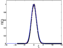
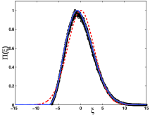
(a)	(b)
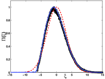
(c)	(d)

Figure 1: The distribution of fluctuations at distinct rescaled times $\tau$. The snapshots refer to: (a) $\tau=5$, (b) $\tau=36$, (c) $\tau=41$ and (d) $\tau=50$. The symbols stand for direct stochastic simulations. The solid lines represent the theoretical predictions as obtained within the generalized Fokker Planck scenario. We have in particular truncated the sums in the Fokker-Planck (Non-Gaussian fluctuations in stochastic models with absorbing barriers) to $k=3$ ($1/N^{3/2}$ corrections) and included $200$ moments in the final estimates of the generating function. The dashed lines refer to the Gaussian solutions obtained working within the van Kampen expansion at the, conventional, next to leading approximation ($1/N^{1/2}$ terms). Here $\nu=0.01$ and the distributions are normalized so to have the maximum equal to one.

To progress with the calculation, we set off to estimate the moments of the sought distribution $\Pi(\xi,\tau)$. Let us recall that the moment of order $h$ is defined as

$$\langle\xi^{h}\rangle=\int_{-\infty}^{\infty}\Pi(\xi)\xi^{h}d\xi.$$

Multiply both sides of the generalized Fokker-Planck equation by the factor $\xi^{h}$ and integrate over $\mathbb{R}$ in $d\xi$. A straightforward manipulation yields to:

$$\frac{d}{d\tau}\langle\xi^{h}\rangle=$$

$$+\sum_{k=1}^{h-2}\frac{1}{(k+1)!}\frac{f(\phi,k+1)}{N^{(k-1)/2}}\frac{h!(-1)^{k+1}}{(h-(k+1))!}\langle\xi^{h-(k+1)}\rangle$$

$$+\sum_{k=1}^{h-1}\frac{1}{k!}\frac{g(\phi,\xi,k)}{N^{(k-1)/2}}\frac{h!(-1)^{k}}{(h-k)!}\langle\xi^{h-k+1}\rangle$$ (4)

$$+\sum_{k=3}^{h+2}\frac{1}{(k-1)!}\frac{q(\xi^{2},k-1)}{N^{(k-1)/2}}\frac{h!(-1)^{k-1}}{(h-(k-1))!}\langle\xi^{h-(k-1)+2}\rangle$$

where use has been made of the supposed regularity of the distribution $\Pi(\xi,\tau)$ to drop out the boundary terms resulting from integrating by parts .

We therefore dispose of a closed system of first oder differential equations for the moments of the distribution $\Pi(\xi,\tau)$. We can integrate it numerically and so estimate the quantities $\langle\xi^{h}\rangle$, for all $h$, at any time $\tau$. The knowledge of the moments enables us to immediately reconstruct the characteristic function, and so recover, upon Fourier transform inversion, the distribution $\Pi(\xi,\tau)$. The predicted profiles are displayed in Fig. 1 (solid line) for different times. A comparison is drawn with the outcome of direct stochastic simulations based on the exact Gillespie algorithm Gillespie (1976) (symbols), returning excellent agreement. The distribution of fluctuations displays clear non-Gaussian traits. It gets in fact more and more skewed as time progresses, reflecting the non trivial interplay with the absorbing boundary. Surprisingly, and at odds with what customarily believed, the van Kampen ansatz proves accurate well beyond the Gaussian approximation that is often invoked to justify its intrinsic validity. As a corollary, it seems tempting to argue that the transformation (2) from discrete to continuum variables is an exact one, and not just an approximation that presumably descends from the central limit theorem, as occasionally speculated.

It is also very instructive to analyze the asymptotic fate of the distribution of fluctuations, as predicted within the realm of the van Kampen theory. Based on intuition, we expect that when time goes to infinity, the distribution $\Pi(\xi,\tau)$ converges to a Dirac delta centered in zero. Indeed, plugging into the moments’ equations (Non-Gaussian fluctuations in stochastic models with absorbing barriers), the asymptotic mean-field solution $\phi=0$, and looking for stationary solutions of the obtained system (i.e. setting the derivatives to zero), one readily gets $\langle\xi^{h}\rangle=0$ $\forall h$, the moments of a delta function. However, for times large enough that $\phi\simeq 0$, but before the system has relaxed to its stationary state, the generalized Fokker-Planck equation (Non-Gaussian fluctuations in stochastic models with absorbing barriers) reads:

$$\frac{\partial\Pi}{\partial\tau}=\nu\frac{\partial}{\partial\xi}\left(\xi\Pi\right)+\frac{2-\nu}{2\sqrt{N}}\frac{\partial^{2}}{\partial^{2}\xi}\left(\xi\Pi\right)$$ (5)

where we have only retained the term in $1/\sqrt{N}$ dropping higher orders corrections. Perform now the scaling $\xi\rightarrow\xi^{\prime}/\sqrt{(}N)$. The equation (5) can be cast in the form:

$$\frac{\partial\Pi}{\partial\tau}=\nu\frac{\partial}{\partial\xi^{\prime}}\left(\xi^{\prime}\Pi\right)+\frac{2-\nu}{2}\frac{\partial^{2}}{\partial^{2}\xi^{\prime}}\left(\xi^{\prime}\Pi\right)\quad.$$ (6)

The large time distribution $\Pi(\xi^{\prime},\tau)$ is therefore insensitive to the system size $N$ and bears consequently universal traits. Equation (6) can be solved analytically (see also Di Patti et al. (2011)) to give:

$$\Pi(\xi^{\prime},\tau) = \frac{2\nu}{2-\nu}\frac{1}{1-e^{-\nu\tau}}\exp\left[\frac{2\nu(\xi^{\prime}+\xi^{\prime}_{0}e^{-\nu\tau})}{(2-\nu)(1-e^{-\nu\tau})}\right]$$ (7)

$$\times \left(\frac{\xi^{\prime}}{\xi^{\prime}_{0}}e^{\nu\tau}\right)^{-\frac{1}{2}}I_{1}\left(\frac{4\nu\sqrt{\xi^{\prime}_{0}\xi^{\prime}e^{\nu\tau}}}{(2-\nu)(e^{\nu\tau}-1)}\right)$$

where $I_{1}(\cdot)$ is the modified Bessel function of the first kind. For large $\tau$, recalling that $I_{1}(x)\simeq x/2$ when $x$ is small, one can approximate Eq. (7) as:

$$\Pi(\xi^{\prime},\tau)\propto\xi_{0}^{\prime}\left(\frac{2\nu}{2-\nu}\right)^{2}\exp(-\frac{2\nu}{2-\nu}\xi^{\prime})\exp(-\nu\tau)$$ (8)

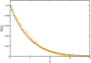
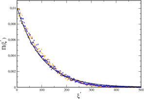
(a)	(b)

Figure 2: The distribution of fluctuations at large times. Left panel: the distribution $\Pi(\xi,\tau)$ is plotted versus $\xi$ at $\tau=388$. Symbols refer to the simulations ($N=1000$), while the solid line stands for the (normalized) solution (8) after the change of variable $\xi^{\prime}\rightarrow\xi\sqrt{(}N)$ is performed. Right panel: the distribution $\Pi(\xi^{\prime},\tau)$ is plotted as function of the rescaled $\xi^{\prime}$. Symbols refer to numerical simulations relative to distinct $N$. In particular, $N=500$ (circles) and $N=1000$ (triangles). The solid line stands for the (normalized) solution (8). Here $\nu=0.01$ and the distributions are normalized to unit.

Operating with the rescaled variable $\xi^{\prime}$, which, it is worth emphasizing, emerges naturally within the van Kampem expansion, when the large time limit is being considered, it is equivalent to inserting into the governing master equation the modified ansatz $n=N\phi+\xi^{\prime}$. This latter corresponds to the strategy adopted in Di Patti et al. (2011) for the specific choice $\alpha=0$. In other words, and interestingly enough, the expected fluctuations $\xi^{\prime}$ are comparable to the discrete population size $n$, when the absorbing boundary is being approached. We have therefore recovered exactly the same solution as obtained in Di Patti et al. (2011), while working within the generalized, but conventional, van Kampen approach. The adequacy of (8) is challenged in Fig. 2 versus numerical simulations returning a perfect quantitative agreement. Notice that different distribution profiles recorded at distinct values $N$, nicely superpose when the rescaled fluctuations $\xi^{\prime}$ is employed.

As a side remark, we stress that the same conclusion can be drawn working in the Fourier space and operating under analogous approximations. Retaining only $1/\sqrt{N}$ corrections in (Non-Gaussian fluctuations in stochastic models with absorbing barriers), assuming $\phi\rightarrow 0$ and performing the scaling $\langle\eta^{h}\rangle=\langle\xi^{h}\rangle N^{\frac{h}{2}}$, one immediately obtains the following $N$ independent differential equations for the moments evolution:

$$\frac{\partial}{\partial\tau}\langle\eta^{h}\rangle=-\nu h\langle\eta^{h}\rangle+\frac{h(h-1)}{2}(2-\nu)\langle\eta^{h-1}\rangle.$$ (9)

Equations (9), here obtained within the extended van Kampen scenario, could be also derived via the alternative, supposedly distinct, approach discussed in Di Patti et al. (2011). Equations (9) can be in fact straightforwardly deduced from Eq. (6) (see also Eq. (8) in Di Patti et al. (2011)) following the same strategy for the evaluation of the moments as outlined above.

In conclusion, the van Kampen approximation works effectively for all times, well beyond the Gaussian approximation and in a regime where the presence of the absorbing boundary is definitely important. The method returns in fact the correct asymptotic solution (a delta function centered in the origin), but also converges to the large time solution calculated in Di Patti et al. (2011), which is therefore contextualized within a general descriptive picture. At moderate times, after the Gaussian approximation has broken down, direct comparisons with the numerical experiments, as reported in this Letter, testify on the excellent predictive ability of the van Kampen theory. This is an important observation, that will certainly motivate using the van Kampen machinery beyond the limited domains of applications for which it was originally conceived, and/or later referred to Di Patti et al. (2011). Future investigations will be targeted to extending the current analysis to cases where the absorbing boundary competes with a non trivial stable fixed point, as well as models for which the notion of space is explicitly accounted for de Anna et al. (2010); Lugo and McKane (2008).

References

- McKane and Newman (2005) A. J. McKane and T. J. Newman, PRL 94, 218102 (2005).
- Dauxois et al. (2009) T. Dauxois, F. Di Patti, D. Fanelli, and A. J. McKane, PRE 79, 036112 (2009).
- de Anna et al. (2010) P. de Anna, F. Di Patti, A. J. McKane, and T. Dauxois, PRE 81, 056110 (2010).
- Biancalani et al. (2010) T. Biancalani, D. Fanelli, and F. Di Patti, PRE 81, 046215 (2010).
- Gardiner (1985) C. W. Gardiner, Handbook of Stochastic Methods, 2nd ed. (Springer, 1985).
- van Kampen (1992) N. G. van Kampen, Stochastic preocesses in Physics and Chemistry (North Holland, Amsterdam, 1992).
- Di Patti et al. (2011) F. Di Patti, S. Azaele, J. R. Banavar, and A. Maritan, PRE 83, 010102(R) (2011).
- Grima (2009) R. Grima, PRL 102, 218103 (2009).
- Pawula (1967a) R. F. Pawula, Physical Review 162, 186 (1967a).
- Pawula (1967b) R. F. Pawula, IEEE Transaction on Information Theory 13, 33 (1967b).
- Risken and Vollmer (1979) H. Risken and H. D. Vollmer, Zeitschrift für Physik B 35, 313 (1979).
- Gillespie (1976) D. T. Gillespie, J. Comp. Phys. 22, 403 (1976).
- Lugo and McKane (2008) C. A. Lugo and A. J. McKane, PRE 78, 051911 (2008).