Non-axisymmetric instabilities of neutron star with toroidal magnetic fields

Abstract

Context. Neutron stars with strong toroidal magnetic fields are often produced in nature. We show that isentropic neutron stars with purely toroidal magnetic fields are unstable against the interchange, Parker and/or Taylor instabilities irrespective of the toroidal magnetic field configurations.

Aims. The aim of this paper is to clarify the stabilities of neutron stars with strong toroidal magnetic fields against non-axisymmetric perturbation. The motivation comes from the fact that super magnetized neutron stars of $\sim 10^{15}$G, magnetars, and magnetized proto-neutron stars born after the magnetically-driven supernovae are likely to have such strong toroidal magnetic fields.

Methods. Long-term, three-dimensional general relativistic magneto-hydrodynamic simulations are performed, preparing isentropic neutron stars with toroidal magnetic fields in equilibrium as initial conditions. To explore the effects of rotations on the stability, simulations are done for both non-rotating and rigidly rotating models.

Results. We find the emergence of the Parker and/or Tayler instabilities in both the non-rotating and rotating models. For both non-rotating and rotating models, the Parker instability is the primary instability as predicted by the local linear perturbation analysis. The interchange instability also appears in the rotating models. It is found that rapid rotation is not enough to suppress the Parker instability, and this finding does not agree with the perturbation analysis. The reason for this is that rigidly and rapidly rotating stars are marginally stable, and hence, in the presence of stellar pulsations by which the rotational profile is deformed, unstable regions with negative gradient of angular momentum profile is developed. After the onset of the instabilities, a turbulence is excited. Contrary to the axisymmetric case, the magnetic fields never reach an equilibrium state after the development of the turbulence.

Conclusions. Isentropic neutron stars with strong toroidal magnetic fields are likely to be always unstable against the Parker instability. A turbulence motion is induced and maintained for a long time. This conclusion is different from that in axisymmetric simulations and suggests that three-dimensional simulation is indispensable for exploring the formation of magnetars or prominence activities of magnetars such as giant flares.

1 Introduction

There are a lot of observational evidences that suggest the presence of neutron stars with strong magnetic fields. Observed spin periods and their time derivatives in conjunction with the assumption of a magnetic dipole radiation give us magnetic field strength as $B\propto(P\dot{P})^{1/2}$ where $P$ and $\dot{P}$ are the spin period and its derivative, respectively. For radio pulsars, of which more than 1800 are known today (Manchester et al. 2005), the inferred value of the magnetic field strength is in the range $10^{11}$–$10^{14}$ G. For a smaller population of older, millisecond pulsars, the typical magnetic field strength is $B\sim 10^{8}$–$10^{9}$ G. For anomalous X-ray pulsars (AXPs) and soft gamma repeaters (SGRs), super strong magnetic fields of $10^{14}-10^{15}$ G are again inferred from the measured values of $P$ and $\dot{P}$ (Woods & Thompson 2004). Various observed properties of AXPs and SGRs like the giant flares from the three SGRs and bursts are often explained in connection with a super strong magnetic field (Thompson & Duncan 1995, 1996, 2001) rather than with rotation because their spin down luminosities are much smaller than the observed luminosity. In addition, temporary detections of spectral lines during SGR/AXP bursts have been reported in several systems (Gavriil et al. 2002; Ibrahim et al. 2003; Rea et al. 2003). If we assume that they are associated with proton cyclotron lines, the magnetic field strength is estimated to give $B\sim 10^{15}$ G.

For about a dozen accreting X-ray pulsars in binary systems, electron cyclotron line features have been detected, suggesting that $B\sim 10^{12}-10^{13}$ G according to the formula for the electron cyclotron energy, $E_{\rm ce}=\hbar B/(m_{e}c)=11.58(B/10^{12}\leavevmode\nobreak\ {\rm G})$ keV  (Orlandini & Fiume 2001). For many other X-ray pulsars with no detectable electron cyclotron line features, typical magnetic fields are $B\sim 10^{12}$ G if one assumes that spin up due to accretion of matter is balanced by magnetic braking (Bildsten et al. 1997).

From a theoretical point of view, these strongly magnetized objects deserve a detailed study, because their magnetic fields sometimes exceed the quantum critical field strength, $B_{\rm QED}=m_{e}^{2}c^{3}/(e\hbar)=4.144\times 10^{13}$ G, at which gyration radius of the electron $pc/(eB)$ is shorter than the de Broglie wavelength $\hbar/p$. Above this limit, magnetic fields affect the properties of atoms, molecules, and condensed matters (Lai 2001), propagation of photons, radiative processes, equation of states, and thermal conductivity in crusts (see Harding & Lai (2006) and references therein). The origin of such extremely large magnetic fields has been a big issue since their discovery. Specifically, there are two hypotheses for its origin; in one scenario, the magnetic fields are assumed to be generated in a rapidly rotating proto-neutron star formed after stellar core collapse of a massive star (Thompson & Duncan 1993) and in the other, it is assumed to be descended from the main sequence stars, i.e., the strong magnetic field is assumed to be a fossil of a strongly magnetized main sequence star (Wickramasinghe & Ferrario 2005). For exploring the magnetar formation, there are a plenty of magneto-hydrodynamic simulations for supernova core collapse both in Newtonian gravity (Yamada & Sawai 2004; Kotake et al. 2004; Obergaulinger et al. 2006; Scheidegger et al. 2008; Takiwaki et al. 2009; Burrows et al. 2007), and in general relativity (Shibata et al. 2006; Cerda-Duran et al. 2007). For these works, the simulations were performed in axisymmetric spacetime. In most of these simulations, it was found that toroidal magnetic fields are dominantly enhanced in the proto-neutron stars after the core bounce by the magnetic winding mechanism, and eventually, the proto-neutron star settles to a quasi-equilibrium state. However, it has been well known that purely toroidal fields in equilibria are often unstable due to the interchange, Tayler, and Parker instabilities (Acheson 1978; Goossens 1980; Parker 1955, 1966; Tayler 1973). The stability analyses have suggested that non-axisymmetric modes would play an essential role for these instabilities and rapid rotation could suppress these instabilities (Acheson 1978).

Motivated by these facts, we studied the axisymmetric instability of neutron stars with toroidal magnetic fields in the previous work (Kiuchi et al. 2008). In that work, magnetized neutron stars in equilibria are prepared as initial conditions with varying its profile and strength and with changing the angular velocity (Kiuchi & Yoshida 2008). Performing the general relativistic magneto-hydrodynamic (GRMHD) simulations, we found that slowly rotating neutron stars with the toroidal fields, whose profile is proportional to the power of cylindrical radius $\varpi$ as $B_{(\varphi)}\propto\varpi^{2k-1}$ with $k\geq 2$, are unstable. The growth time scale is of order the Alfvén time scale, and the type of the instability is the interchange instability in the absence of stellar rotation. Only for the case $k=1$, slowly rotating neutron stars are stable against the axisymmetric perturbation, and thus, we concluded that the configuration with $k=1$ will be the attractor for the unstable neutron stars. We also found that rapid rotation, with which the rotational kinetic energy is much greater than the magnetic energy, suppresses the onset of the interchange instability, and stabilizes the neutron stars. These results qualitatively and semi-quantitatively agree with the local linear analysis.

In the magneto-rotational explosion scenarios, the magnetic energy is composed primarily of the toroidal field and is at most as large as the rotational kinetic energy. This indicates that the axisymmetric interchange instability would not play an important role in the proto-neutron star. However, it is still possible that the neutron star becomes unstable against the Parker and Tayler instabilities which grow in a non-axisymmetric way. Stability of magnetars is also the important issue along this line (Braithwaite & Nordlund 2005; Braithwaite & Spruit 2004). For the magnetar, the rotational effect is negligible. Thus, the toroidal field profile should be similar to that of $k=1$ to avoid the onset of the axisymmetric interchange instability. However, such configuration may be still unstable if the Parker and/or Tayler instabilities are taken into account.

Motivated by these facts, we extend our previous work (Kiuchi et al. 2008). The main aim of this article is to explore the non-axisymmetric instabilities of neutron stars with toroidal magnetic fields. Following our previous work, we prepare equilibrium neutron stars with purely toroidal magnetic fields as initial conditions. This time, we perform three-dimensional GRMHD simulations with varying the field strength and/or rotation velocity. As mentioned above, the three-dimensional simulation is inevitable for exploring the Parker and Tayler instabilities.

This paper is organized as follows. In Section 2, we briefly review the formulation and numerical methods employed in our numerical-relativity simulation. Set up of numerical simulation and initial models for our GRMHD simulations are described in Section 3. In Section 4, we present the results of a local linear perturbation analysis as a forecast of numerical-simulation results. Section 5 is devoted to presenting the numerical results. A summary and discussion are given in Section 6.

Throughout this paper, we adopt the geometrical units in which ${\rm c}={\rm G}=1$ with c and G being the speed of light and gravitational constant, respectively. Cartesian coordinates are denoted by $x^{k}=(x,y,z)$. The coordinates are oriented so that the rotation axis is along the $z$-direction. We define the coordinate radius $r=\sqrt{x^{2}+y^{2}+z^{2}}$, cylindrical radius $\varpi=\sqrt{x^{2}+y^{2}}$, and azimuthal angle $\varphi=\tan^{-1}(y/x)$. Coordinate time is denoted by $t$. Greek indices $\mu,\nu,\cdots$ denote spacetime components, and small Latin indices $i,j,\cdots$ denote spatial components.

2 Formulation and Method

The stability of magnetized neutron stars are studied by three dimensional GRMHD simulation assuming that the ideal MHD condition holds. In this paper we focus on the Parker and/or Tayler instabilities against non-axisymmetric perturbations. The simulation is performed upgrading our axisymmetric GRMHD numerical code in Shibata & Sekiguchi (2005); Kiuchi et al. (2008) to that for three dimensions.

Formulation and numerical scheme for solving Einstein’s equation are essentially the same as in Shibata & Nakamura (1995). For solving Einstein’s evolution equation, we use the original version of the Baumgarte-Shapiro-Shibata-Nakamura formulation (Shibata & Nakamura 1995; Baumgarte & Shapiro 1999): We evolve the inverse square of the conformal factor $W\equiv\exp(-2\phi)$ with $\phi=\ln(\gamma)/12$, the trace part of the extrinsic curvature, $K$, the conformal three-metric, $\tilde{\gamma}_{ij}\equiv\gamma^{-1/3}\gamma_{ij}$, the tracefree extrinsic curvature, $\tilde{A}_{ij}\equiv\gamma^{-1/3}(K_{ij}-K\gamma_{ij}/3)$, and a three-auxiliary variable, $F_{i}\equiv\delta^{jk}\partial_{j}\tilde{\gamma}_{ik}$. Here, $\gamma_{ij}$ is the three-metric, $K_{ij}$ the extrinsic curvature, $\gamma\equiv{\rm det}(\gamma_{ij})$, and $K\equiv K_{ij}\gamma^{ij}$. Note that we evolve $W$, not the conformal factor as in Kiuchi et al. (2009), because our code is designed to simulate black hole spacetimes with the moving puncture method (Baker et al. 2006; Campanelli et al. 2006; Brugmann et al. 2008). For the conditions of the lapse, $\alpha$, and the shift vector, $\beta^{i}$, we adopt a dynamical gauge condition in the following forms (Shibata 2003),

$$(\partial_{t}-\beta^{i}\partial_{i})\ln\alpha=-2K,$$ (1)

$$\partial_{t}\beta^{i}=0.75\tilde{\gamma}^{ij}(F_{j}+\Delta t\partial_{t}F_{j}),$$ (2)

where $\Delta t$ denotes the time step in the numerical simulations, and the second term in the right-hand side of (2) is introduced for stabilizing the numerical computations. The finite-differencing schemes for solving Einstein’s equation is essentially the same as those in Kiuchi et al. (2009). We use the fourth-order finite-differencing scheme in the spatial direction and a fourth-order Runge-Kutta scheme in the time integration, where the advection terms such as $\beta^{i}\partial_{i}W$ are evaluated by a fourth-order non-centered difference scheme, as proposed, e.g., in Brugmann et al. (2008).

A conservative shock-capturing scheme is employed to integrate the GRMHD equations. Specifically we use a high-resolution central scheme (Kurganov & Tadmor 2000; Lucas-Serrano et al. 2004) with the third-order piece-wise parabolic interpolation and with a steep min-mod limiter in which the limiter parameter $b$ is set to be 2.5 (see appendix A of Shibata (2003)).

Magnetized neutron stars in equilibrium, employed as the initial condition, are computed giving the polytropic equation of state (Kiuchi & Yoshida 2008),

$$P=\kappa\rho^{\Gamma},$$ (3)

where $P$, $\rho$, $\kappa$, and $\Gamma$ are the pressure, rest-mass density, polytropic constant, and adiabatic constant, respectively. In this work, we choose $\Gamma=2$. Because $\kappa$ is arbitrarily chosen or else completely scaled out of the problem, we adopt the units of $\kappa=1$ in the following (i.e., the polytropic units of c$=$G=$\kappa=1$ are employed). In the numerical simulation, we adopt the $\Gamma$-law equation of state as

$$P=(\Gamma-1)\rho\varepsilon,$$ (4)

where $\varepsilon$ is the specific internal thermal energy.

We monitor the total baryon rest mass $M_{b}$, Arnowitt-Deser-Misner (ADM) mass $M$, internal energy $U_{\rm int}$, rotational kinetic energy $T_{\rm rot}$, total kinetic energy $T_{\rm kin}$, and magnetic energy $H_{\rm mag}$, defined by

$$M_{b}=\int\rho w\sqrt{\gamma}d^{3}x$$ (5)

$$M=\int e^{-\phi}\Big{[}\rho hw^{2}-P+\frac{1}{16\pi}\{K_{ij}K^{ij}-K^{2}-\tilde{R}e^{-4\phi}\}\Big{]}\sqrt{\gamma}d^{3}x$$ (6)

$$U_{\rm int}=\int\rho w\varepsilon\sqrt{\gamma}d^{3}x$$ (7)

$$T_{\rm rot}=\frac{1}{2}\int\rho hwu_{\varphi}\Omega\sqrt{\gamma}d^{3}x$$ (8)

$$T_{\rm kin}=\frac{1}{2}\int\rho hwu_{i}v^{i}\sqrt{\gamma}d^{3}x$$ (9)

$$H_{\rm mag}=\frac{1}{8\pi}\int b^{2}w\sqrt{\gamma}d^{3}x$$ (10)

where $\tilde{R}$ is the Ricci scalar with respect to $\tilde{\gamma}_{ij}$, $u^{\mu}$ is the four velocity of the fluid, $h$ is the specific enthalpy defined by $1+\varepsilon+P/\rho$, $w\equiv\alpha u^{t}$, $v^{i}=u^{i}/u^{t}$, $\Omega=v^{\varphi}$, and $b^{2}=b^{\mu}b_{\mu}$. $b^{\mu}$ is the magnetic field observed in the frame co-moving with the fluid element. $M_{0}$ denotes the initial value of the ADM mass. Once each energy component is obtained, we define the gravitational potential energy by

$$W=M-(M_{b}+U_{\rm int}+T_{\rm kin}+H_{\rm mag}).$$ (11)

Following Kiuchi et al. (2008), we define an averaged Alfvén time scale as

$$\bar{v}_{A}\equiv\sqrt{\frac{2H_{\rm mag}}{M_{b}+\Gamma U_{\rm int}+2H_{\rm mag}},}$$ (12)

where we use the relation $h=1+\Gamma\varepsilon$, which holds in the $\Gamma$-law equation of state. Note that the Alfvén velocity in relativity is given by $\sqrt{b^{2}/(4\pi\rho h+b^{2})}$. Then, we define the averaged Alfvén time scale as

$$\bar{\tau}_{A}\equiv\frac{R}{\bar{v}_{A}},$$ (13)

where $R$ is the equatorial stellar radius. Because the magnetic field instability grows on an order of the Alfvén time scale (cf. Section 4), $\bar{\tau}_{A}$ is useful to judge whether or not the instability found in numerical simulation is associated with a magnetic field effect.

3 Model and Numerical setup

3.1 Initial condition

Neutron stars with toroidal magnetic fields in equilibrium, employed as initial conditions, are computed by the code described in Kiuchi & Yoshida (2008). Several key quantities characterizing these magnetized neutron stars are listed in Table 1. The instability associated with the presence of toroidal magnetic fields depends on the profile of the magnetic field as shown by Acheson (1978); Goossens (1980); Spruit (1999); Tayler (1973). We assume the toroidal magnetic field profile confined inside the neutron star to be given by

$$b_{(\varphi)}=B_{0}u^{t}(\rho h\alpha^{2}\gamma_{\varphi\varphi})^{k}\gamma_{\varphi\varphi}^{-1/2},$$ (14)

where $k$ and $B_{0}$ are constants which determine the field profile and strength, respectively. The regularity condition of magnetic fields near the axis of $\varpi=0$ requires $k\geq 1$. Because of $\gamma_{\varphi\varphi}\propto\varpi^{2}$ for $\varpi\rightarrow 0$, the toroidal magnetic field is proportional to $\varpi^{2k-1}$ near the axis. Previous works predict that the profile with $k\geq 2$ is unstable against axisymmetric perturbations (Acheson 1978; Goossens 1980; Spruit 1999; Tayler 1973) and we confirmed this prediction in the previous paper (Kiuchi et al. 2008). On the other hand, the profile of $k=1$ is not unstable against axisymmetric perturbations but may be unstable against non-axisymmetric ones (see also Lander et al. (2010); Lander & Jones (2010)). Hence in this paper, we focus on the profile of $k=1$.

Magnetic field strength, $B_{0}$, is chosen so as to satisfy $8\times 10^{-3}\leq H/|W|\leq 5\times 10^{-2}$. These values imply the field strength of $10^{16}$–$10^{17}\leavevmode\nobreak\ {\rm G}$ for a typical neutron star of mass $1.4M_{\odot}$, radius $10\leavevmode\nobreak\ {\rm km}$, and $|W|\sim 6\times 10^{53}\leavevmode\nobreak\ {\rm erg}$. These magnetic field strengths are extremely large even for models of magnetar and might be less realistic. We here give such strong magnetic fields simply to save the computational costs; note that the growth time scales of the instabilities by the presence of the toroidal magnetic field are of order Alfvén time scale, which is still much longer than the dynamical time scale of the system in the present set up. Thus, a scaling relation should hold for a weaker magnetic field strength. We may apply the scaling relation to derive a generic physical essence from the results obtained in the present set up. Namely, if the magnetic field strength becomes half, the growth time scale of the instabilities becomes approximately twice longer, although qualitative properties of the evolution of the unstable neutron star are essentially the same.

The initial conditions for the non-rotating model is specified if the central density $\rho_{c}$ (in the polytropic units) is determined. We choose it to be $\rho_{c}\approx 0.22$. With this choice, the neutron star has a realistic compactness; e.g, if we assume $M\approx 1.35M_{\odot}$, circumferential radius is $R\approx 11$km (cf. Table 1). Note that the maximum rest mass and gravitational mass of the spherical neutron star for $\Gamma=2$ are, respectively, $0.1799$ and $0.1637$, and the corresponding central density is $\approx 0.318$ in our unit.

Simulations are also performed for rotating neutron star models. In this paper, we focus only on rigidly rotating neutron stars with a moderate compactness; $\rho_{c}$ is again chosen to be $0.22$. For the neutron stars with the $\Gamma=2$ polytrope, the maximum values of $T_{\rm rot}/|W|$ is $\sim 0.09$ for $M_{0}/R_{\rm cir}\sim 0.1$ (Cook et al. 1994). Local linear stability analysis predicts that rapid rotations will suppress the growth of some of the instabilities associated with the presence of toroidal magnetic fields (Acheson (1978), see also Section 4.2). To study whether this would be indeed the case, we prepare rapidly rotating models with $T_{\rm rot}/|W|\approx 0.08$, and vary the magnetic field strength.

3.2 Grid settings

The simulations are performed on the cell-centered Cartesian, $(x,y,z)$, grid. Equatorial plane symmetry with respect to $z=0$ plane is assumed. The computational domain of $-L\leq x\leq L$, $-L\leq y\leq L$, and $0\leq z\leq L$ is covered by the grid size $(2N,2N,N)$ for $(x,y,z)$, where $L$ and $N$ are constants. Following Kiuchi et al. (2008), we adopt a non-uniform grid as follows; an inner domain is covered with an uniform grid of spacing $\Delta x$ and with the grid size, $(2N_{0},2N_{0},N_{0})$. Outside this inner domain, the grid spacing is increased according to the relation, $\xi\tanh[(i-N_{0})/\Delta i]\Delta x$, where $i$ denotes the $i$-th grid point in each positive direction, and $N_{0}$, $\Delta i$, and $\xi$ are constants. Then, the location of $i$-th grid, $x^{k}(i)$ ($i\geq 0$), for each direction is

$$x^{k}(i)=\left\{\begin{array}[]{ll}(i+1/2)\Delta x&i\leq N_{0}\\ (i+1/2)\Delta x+\xi\Delta i\Delta x\log[\cosh\{(i-N_{0})/\Delta i\}]&i>N_{0}\\ \end{array}\right.$$ (17)

and $x^{k}(-i-1)=-x^{k}(i)$, where $i=0,1,\cdots N-1$ for $x^{k}=x,y,$ and $z$. The chosen parameters of the grid structure for each simulation are listed in Table 2. To check the validity of our numerical results, the simulations for models N22H5 and R22H2T8 are performed with three different grid resolutions. With the highest (lowest) resolution, the coordinate equatorial radii of neutron stars, $L_{\rm NS}$, are covered by 130 (80) grid points while the outer boundary location is chosen to be $\simeq 8L_{\rm NS}$ in all the simulations. We confirmed the modest resolution in which $L_{\rm NS}$ is covered by 100 grid points is high enough to draw a resolution-invariant conclusion.

Table 1: List of characteristic quantities for neutron stars with toroidal magnetic fields.

Model	$\rho_{c}$	$U_{\rm int}/|W|$	$H_{\rm mag}/|W|$	$T_{\rm rot}/|W|$	$M_{0}$	$M_{\rm b}$	$M_{0}/R_{\rm cir}$	$\bar{\tau}_{A}/M_{0}$
N22H5	2.2E-1 (1.24)	5.12E-1	5.01E-2	0	1.59E-1 (1.67)	1.73E-1 (1.81)	1.78E-1	37.4 (0.31)
N22H1	2.2E-1 (1.24)	5.32E-1	1.01E-2	0	1.60E-1 (1.68)	1.75E-1 (1.96)	1.87E-1	76.7 (0.63)
R22H2T8	2.2E-1 (1.24)	4.71E-1	1.50E-2	7.97E-2	1.84E-1 (1.93)	2.01E-1 (1.63)	1.55E-1	63.5 (0.63)
R22H08T8	2.2E-1 (1.24)	4.74E-1	7.86E-3	8.10E-2	1.85E-1 (1.94)	2.02E-1 (1.73)	1.65E-1	97.3 (0.93)

Table 2: Parameters for the grid structure employed in the numerical simulation.

Model	$N$	$N_{0}$	$\Delta i$	$\xi$	$L_{\rm NS}/\Delta x$
N22H5-l	161	120	30	22	80
N22H5	200	150	30	20	100
N22H5-h	253	195	30	20	130
N22H1	200	150	30	20	100
R22H2T8-l	161	120	30	22	80
R22H2T8	200	150	30	20	100
R22H2T8-h	253	195	30	21	130
R22H08T8	226	180	30	22	100

4 Local linear perturbation analysis

Before showing the results of nonlinear numerical simulation, it is useful to remind the results of linear-stability analysis. By using the local linear perturbation analysis (Acheson 1978), the dispersion relations for the non-rotating and rotating models are derived, and the (local) stability is determined. In the following, the method of the analysis in the Newtonian framework is briefly reviewed.

In the local analysis, a perturbation quantity $\delta Q$ is assumed to be given by

$$\delta Q=Q_{0}\exp[i(l\varpi+m\varphi+nz-\sigma t)],$$ (18)

where $Q_{0}$ is a constant, $\sigma$ is the oscillation frequency, and $(l,m,n)$ is the wave number vector. To obtain the local dispersion relations, we assume that $l\gg 1$, $n\gg 1$, and $m=O(1)$, which implies that perturbations we consider have very short wavelength on the meridional plane (for details, cf. Acheson (1978)).

4.1 Non-rotating case

The dispersion relation for non-rotating models is given, irrespective of the density profile, by

$$\left(1+\frac{l^{2}}{n^{2}}\right)\left(1+\frac{v_{A}^{2}}{c_{s}^{2}}\right)\sigma^{4}$$

$$+\left[v_{A}^{2}\left(\frac{2}{\varpi}-\frac{\hat{G}}{c_{s}^{2}}\right)\partial_{h}\ln\left(\frac{B_{(\varphi)}}{\rho\varpi}\right)-\left(1+\frac{l^{2}}{n^{2}}\right)m^{2}\sigma_{A}^{2}\left(2+\frac{v_{A}^{2}}{c_{s}^{2}}\right)\right]\sigma^{2}$$

$$+\left(1+\frac{l^{2}}{n^{2}}\right)m^{4}\sigma_{A}^{2}+m^{2}\sigma_{A}^{4}\varpi^{2}\left(\frac{\hat{G}}{c_{s}^{2}}-\frac{2}{\varpi}\right)\partial_{h}\ln(B_{(\varphi)}\varpi)=0$$ (19)

where $v_{A}=B_{(\varphi)}/\sqrt{4\pi\rho}$, $\sigma_{A}=v_{A}/\varpi$, $\hat{G}=g_{\varpi}-(l/n)g_{z}$ with $g_{\varpi}$ and $g_{z}$ being the gravitational acceleration, $\partial_{h}=\partial_{\varpi}-(l/n)\partial_{z},$ and $c_{s}$ is the sound speed. For the axisymmetric perturbation, i.e., $m=0$ perturbations, the dispersion relation is reduced to a quadratic form of $\sigma$ as

$$\left(1+\frac{l^{2}}{n^{2}}\right)\left(1+\frac{v_{A}^{2}}{c_{s}^{2}}\right)\sigma^{2}+\left[v_{A}^{2}\left(\frac{2}{\varpi}-\frac{\hat{G}}{c_{s}^{2}}\right)\partial_{h}\ln\left(\frac{B_{(\varphi)}}{\rho\varpi}\right)\right]=0.$$ (20)

For the density profile which is necessary to solve Equation (19) for a specific model, we prepare the Newtonian spherical polytrope with $\Gamma=2$ as

$$\rho=\rho_{0}\frac{\sin(\pi r/r_{s})}{\pi r/r_{s}}$$ (21)

where $\rho_{0}$ and $r_{s}$ are the central density and stellar radius. The spherical density profile is justified by the assumption of a weak magnetic field, i.e., the magnetic field is too weak to deform the star. In the Newtonian limit, Equation (14) becomes

$$B_{(\varphi)}=B_{0}\rho\varpi\,.$$ (22)

Because $B_{(\varphi)}/{\rho\varpi}=$const. in our models (see Equations ((21) and (22)), we have $\sigma=0$ for $m=0$, i.e., the magnetic field is marginally stable against the axisymmetric perturbation. Physically, the magnetic field instability caused by the axisymmetric perturbation is classified as the interchange instability. Our models are marginally stable against such instability and we indeed found in the previous study that they were not unstable (Kiuchi et al. 2008). However, the marginally stable profile is not always kept in a stationary state in the presence of a perturbation. We return to this point in Section 5.2.

For non-axisymmetric perturbations, we forecast that the Parker instability (Parker 1955, 1966) and the Tayler instability (Tayler 1973) set in. Following Acheson (1978), we define the critical radius as

$$\varpi_{c}\equiv\frac{2c_{s}^{2}}{g_{\varpi}}.$$ (23)

Outside this critical radius, the magnetic buoyant force exceeds the magnetic hoop stress, whereas inside it, the magnetic stress is dominant. The Tayler instability could set in near the axis of $\varpi=0$ (Spruit 1999), which is inside the critical radius. On the other hand, the Parker instability could play a role in places where the magnetic buoyancy force surpasses the magnetic tension. Thus, we classify the instability which emerges inside and outside the critical radius as the Tayler and Parker instabilities, respectively. Analyzing the dispersion relation near the axis of $\varpi=0$, Acheson (1978) and Spruit (1999) concluded that the dominant modes of the Tayler instability are $m=1$ and $l/n\approx 0$ modes, which are associated with the horizontal motion near the axis of $\varpi=0$. However, to clarify the most relevant unstable modes, we have to determine the growth time scales of the instability for all the places inside the star. Hence, we calculate the maximum growth rates of the instability solving the dispersion relation (19) with varying $l/n$ and $m$.

Figure 1 displays the contours of the growth rate for the model with $\rho_{0}=0.16$ and $B_{0}=0.2$, which give $H_{\rm mag}/|W|=2.5\%$ and $M_{b}=0.2$ in the polytropic units. These parameters are chosen so as to mimic the initial models shown in Table 1. The white colored region and the dotted curve denote the stable region and critical radius, respectively. We note that the most unstable mode at each point is the $l/n=0$ mode. This figure shows that the fastest growing mode of the instability is located near the stellar surface and is determined by the Parker instability, because the location is outside the critical radius. The right panel of Figure 1 shows that not the $m=1$ mode but a high-order $m$ mode is relevant for this fastest growing mode. The local linear perturbation analysis predicts that the Parker instability primarily emerges near the stellar surface in our non-rotating models.

4.2 Rotating-case

For the rotating models, the dispersion relation is written as

$$\left(1+\frac{l^{2}}{n^{2}}\right)\left(1+\frac{v_{A}^{2}}{c_{s}^{2}}\right)\omega^{4}+\Bigg{[}v_{A}^{2}\partial_{h}\ln\left(\frac{B_{(\varphi)}}{\rho\varpi}\right)\left(\frac{2}{\varpi}-\frac{\hat{G}}{c_{s}^{2}}\right)$$

$$-\left(1+\frac{l^{2}}{n^{2}}\right)m^{2}\sigma_{A}^{2}\left(2+\frac{v_{A}^{2}}{c_{s}^{2}}\right)-\frac{2\Omega}{\varpi}\partial_{h}(\Omega\varpi^{2})\left(1+\frac{v_{A}^{2}}{c_{s}^{2}}\right)\Bigg{]}\omega^{2}$$

$$-\frac{4\Omega mv_{A}^{2}}{\varpi}\left(\frac{2}{\varpi}-\frac{\hat{G}}{c_{s}^{2}}\right)\omega+m^{2}\sigma_{A}^{2}\Bigg{[}2\varpi\Omega\partial_{h}\Omega+\left(1+\frac{l^{2}}{n^{2}}\right)m^{2}\sigma_{A}^{2}$$

$$-\left(\frac{2}{\varpi}-\frac{\hat{G}}{c_{s}^{2}}\right)\partial_{h}\ln(B_{(\varphi)}\varpi)v_{A}^{2}\Bigg{]}=0,$$ (24)

where $\omega=\sigma-m\Omega$ with $\Omega$ being the angular velocity. Following Acheson (1978), we focus on a low-frequency and non-axisymmetric mode, for which the growth time scale is much longer than the Alfvén time scale as

$$|\omega|^{2}\ll m^{2}\sigma_{A}^{2}.$$ (25)

We also adopt a weak magnetic field approximation in which magnetic energy is assumed to be everywhere much smaller than the rotational kinetic energy as

$$v_{A}^{2}\ll\Omega^{2}\varpi^{2}.$$ (26)

With these approximations, the bi-quadratic equation (24) is reduced to a quadratic equation and its solution is

$$\omega=\left(\frac{\hat{G}}{c_{s}^{2}}-\frac{2}{\varpi}\right)\frac{mv_{A}^{2}}{2\Omega\varpi}\pm\frac{mv_{A}}{2\Omega\varpi}\Bigg{[}\left(\frac{\hat{G}}{c_{s}^{2}}-\frac{2}{\varpi}\right)v_{A}^{2}\partial_{h}\ln\left(\frac{B_{(\varphi)}}{\rho\varpi}\right)$$

$$\leavevmode\nobreak\ \leavevmode\nobreak\ \leavevmode\nobreak\ \leavevmode\nobreak\ \leavevmode\nobreak\ \leavevmode\nobreak\ \leavevmode\nobreak\ \leavevmode\nobreak\ \leavevmode\nobreak\ +\Omega^{2}\varpi\partial_{h}(\ln\Omega^{2})+\frac{m^{2}v_{A}^{2}}{\varpi^{2}}\left(1+\frac{l^{2}}{n^{2}}\right)\Bigg{]}^{1/2}.$$ (27)

This dispersion relation shows that the instability sets in if either of the following criteria is satisfied,

$$-\Omega^{2}\varpi\partial_{\varpi}(\ln\Omega^{2})-\left(\frac{g_{\varpi}}{c_{s}^{2}}-\frac{2}{\varpi}\right)v_{A}^{2}\partial_{\varpi}\ln\left(\frac{B_{(\varphi)}}{\rho\varpi}\right)>m^{2}\sigma_{A}^{2}$$ (28)

$$-\frac{g_{z}v_{A}^{2}}{c_{s}^{2}}\partial_{z}\ln\left(\frac{B_{(\varphi)}}{\rho\varpi}\right)>m^{2}\sigma_{A}^{2}$$ (29)

The inequalities (28) and (29) do not hold for rigidly rotating stars with the magnetic field profile (22). However, the angular velocity profile of any star never remain constant in a strict sense, because the stars in nature usually oscillate around their equilibria which makes a gradient in the angular velocity profile. In the presence of negative angular velocity gradient, the instability criterion (28) may be satisfied because the first term in the left-hand side of Equation (28) can be the most dominant one due to the weakness of the magnetic field as imposed in Equation (26); for a region in which the Alfvén velocity is much smaller than the rotational velocity, a small perturbation in the angular velocity is sufficient for satisfying the inequality (28). We will discuss this issue in Section 5.2 in more detail.

5 Result

5.1 Non-rotating case

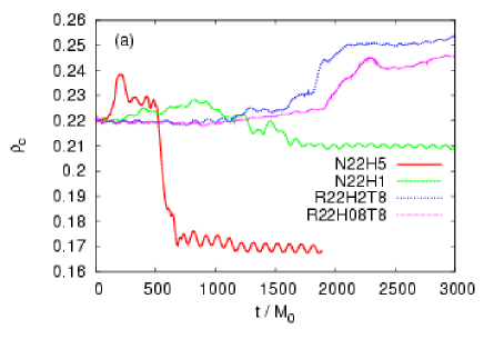
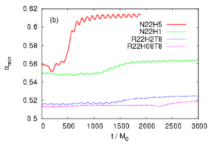
Figure 2: The evolution of (a) central rest-mass density $\rho_{c}$ and (b) minimum value of lapse function $\alpha_{\rm min}$ for non-rotating models N22H1 and N22H5.

We study the stability for two non-rotating models listed in Table 1. The simulations are performed for a sufficiently long time, more than ten times of the averaged Alfvén time scale or several thousands of time in units of $M_{0}$ (cf. Table 1). This is necessary to clarify whether or not any MHD instability, which grows approximately on an Alfvén time scale, sets in and to determine the final fate after the onset of the instabilities. Figure 2 plots the evolution of the central rest-mass density and the minimum value of the lapse function, which characterize the compactness of the neutron star. For the non-rotating model N22H5, it is observed that the central density (the minimum value of the lapse function) increases (decreases) for $t\lesssim 200M_{0}$ and subsequently decreases (increases) for $200M_{0}\lesssim t\lesssim 600M_{0}$ and then stably oscillates for $t\gtrsim 600M_{0}$. This suggests that the star contracts first, then expands slightly, and finally settles to another quasi-equilibrium state with oscillations. Note that the final central density is not beyond the marginally stable point, $\rho_{c}\approx 0.318$. For model N22H1, the qualitative features of the evolution are essentially the same as those of N22H5, but the time scale is different from that of N22H5 because of the difference in the magnetic field strength. The behavior described above is well explained by the variation of magnetic fields during the evolution as argued below.

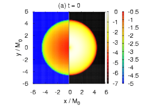
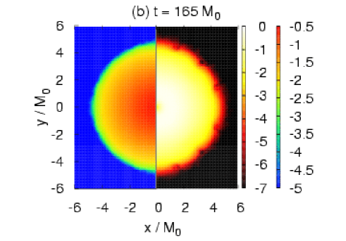
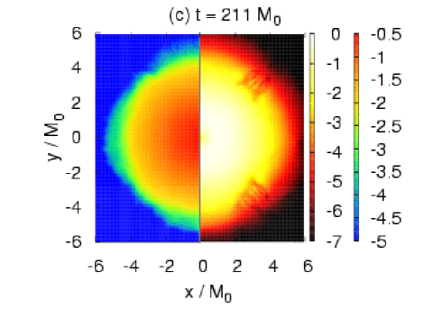
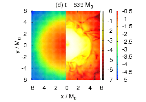
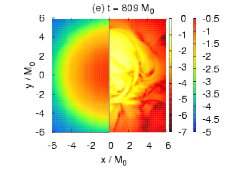
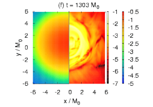
Figure 3: The evolution of rest-mass density (left) and magnetic energy density (right) on the equator for N22H5. Both of them are plotted in the logarithmic scale. The coordinate time at each slice is shown in each panel.

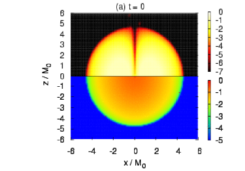
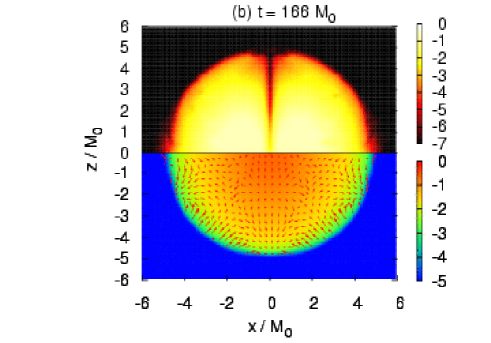
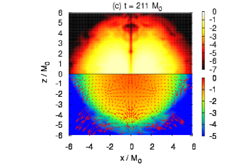
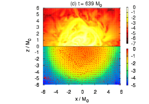
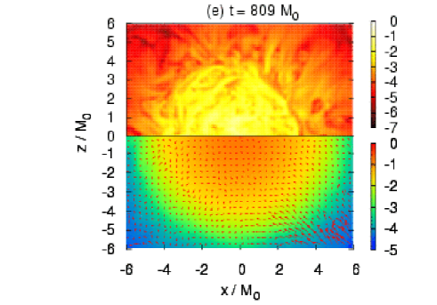
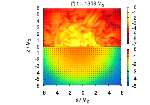
Figure 4: The evolution of the rest-mass density (bottom) and magnetic energy density (top) on a meridian ($x$-$z$) plane for N22H5 in the logarithmic scale. The arrows indicate the velocity fields.

Figures 3 and 4 plot the evolution of the rest-mass density and magnetic energy density on the equatorial plane and in one of meridian ($x$-$z$) planes, respectively, for model N22H5. The panels (a)–(c) in these figures show that the magnetic field near the stellar surface is disturbed by the Parker instability, and leaks out of the stellar surface. Because the plasma beta is small and thus the matter inertia is small near the stellar surface (as shown below), the matter is dragged by the magnetic force and consequently the stellar surface is distorted. Here, the plasma beta is the ratio of the fluid pressure to the magnetic pressure,

$$\beta_{\rm plasma}\equiv\frac{8\pi P}{b^{2}}\propto\frac{\rho^{2}}{b_{(\varphi)}^{2}}\propto\frac{1}{\gamma_{\varphi\varphi}}$$ (30)

where we have used Equations (3) and (14) assuming $\Gamma=2$ and $k=1$. The minimum value of the plasma beta is initially $\approx 2$ at the stellar surface, and after the onset of the Parker instability, the leak-out magnetic field loop produces even lower beta plasma near the stellar surface. As a result, a weak wind expanding outward is driven. On the other hand, the ingoing magnetic field loop enhances a turbulent motion in the neutron star. During the transition from the state shown in panel (c) to (d) in Figures 3 and 4, the initial magnetic field profile is completely destroyed and turbulent magnetic field is produced. During the development of the turbulence, the Tayler instability does not appear to play an important role. However, the region near the axis of $\varpi=0$ is not stable against this instability and thus no mechanism seems to help stabilizing there.

The toroidal magnetic fields initially prepared behave like a rubber belt, which fastens the “waist” of neutron stars. The disappearance of the coherent toroidal magnetic fields, therefore, results in the expansion of the star as shown in the panel (d) of Figures 3 and 4. After the magnetic field becomes turbulent, the star stably oscillates around the hypothetical quasi-stationary state. Although the density profile relaxes to a quasi-stationary state, the turbulent motion is maintained. We observe qualitatively the same features for model N22H1, but the growth time scale of the instability is longer than that of N22H5 as mentioned before.

It is interesting to compare the simulation result with the linear analysis. We find the turbulent field develops in the region which is stable against the perturbation (see the stable region in Figure 1 and Figure 4 (d-f)). During the linear growth phase, i.e., Figure 4 (a-c), this region is likely to be stable. However, because the instability destroys the coherent initial magnetic field profile, i.e., the magnetic field is no longer pure toroidal, the stable region in Figure 1 is no longer stable after the onset of the instability. We also point out that the linear analysis in Figure 1 indicates that the higher $m$ mode is unstable near the stellar surface and we indeed find such a behavior (see Figure 3 (b)). For making the mode growth clear, we perform the mode analysis as follows. Because we are interested in the magnetic field behavior near the surface, we put a ring on the equator whose radius is nearly equal to the stellar radius. Then, the Fourier components are defined by

$$C_{m}=\int^{2\pi}_{0}b^{2}(r_{\rm ring},\pi/2,\varphi){\rm e}^{im\varphi}d\varphi,$$ (31)

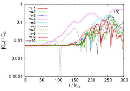
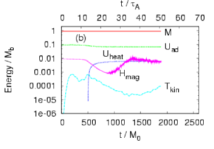
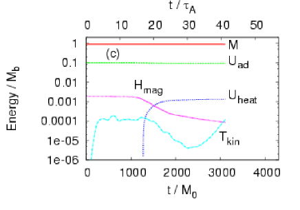
Figure 5: (a) Evolution of the Fourier mode for the magnetic energy density for model N22H5, (b) evolution of several energy components for model N22H5, and (c) the same as (b) but for model N22H1. All the energy components are normalized by the rest mass, and the time axes are shown in units of $M_{0}$ (bottom) and $\bar{\tau}_{A}$ (top). Note that the internal energy is split into the adiabatic and heating parts (see the text for more details).

where $r_{\rm ring}$ is the ring radius which is chosen as $4M_{0}$ for model N22H5. Figure 5 (a) plots the evolution of $|C_{m}|$ with $1\leq m\leq 10$. It is found that all the mode (except for $m=4$ and $8$) start growing at $T\approx 150M_{0}$, that shows that the Parker instabilities are in operation. For $m=4$ and $8$, $|C_{m}|$ starts growing at $T\approx 50M_{0}$. This is the artifact due to our choice of the Cartesian coordinate grid.

The nonlinear growth of the Parker instability is well reflected in the energy components as shown in Figure 5. Here, the internal energy (7) is separated into the adiabatic part $U_{\rm ad}$ and the heating part $U_{\rm heat}$, and they are defined by replacing $\varepsilon$ in Equation (7) to $\varepsilon_{\rm ad}\equiv\rho^{\Gamma-1}/(\Gamma-1)$ and to $\varepsilon-\varepsilon_{\rm ad}$, respectively. Figure 5 shows that the ADM mass is approximately conserved, that implies that gravitational waves are not substantially emitted during the evolution of the neutron stars. The magnetic energy gradually decreases and the kinetic energy increases during $t\lesssim 500M_{0}$ for model H22M5. This illustrates that the meridional circulation is excited due to the instability: Figures 3 and 4 specifically show that this meridional circular motion is induced by the displacement of the toroidal magnetic field line. In other words, the magnetic field helps increasing the kinetic energy of the fluid element by liberating the gravitational potential energy. During this procedure, the kinetic energy eventually reaches about ten percents of the magnetic energy at $t\approx 200M_{0}$.

For $t\gtrsim 500M_{0}$, the decrease rate of the magnetic energy becomes high and simultaneously the thermal energy ($U_{\rm heat}$) quickly increases. This indicates that the shock heating occurs because of the turbulent motion induced by the distorted magnetic fields. The kinetic energy of the circulation gradually decreases, and the magnetic and thermal energies settle approximately to constant values at a late stage of the evolution. The adiabatic internal energy also settles to a value lower than the initial one at $t\approx 500M_{0}$. This implies that the density distribution changes, as shown in Figures 3 and 4. As we pointed out above, however, the magnetic field configuration never reaches to any equilibrium state in contrast to the axisymmetric case (Kiuchi et al. 2008).

All the features found in the evolution of the energy components for model N22H1 are essentially the same as for model N22H5 except for the relevant time scale, as found from Figures 2 and 5. The variation time scales of the various components of the energy for model N22H5 are systematically shorter than those for model N22H1. This is natural because the instability develops approximately in the Alfvén time scale.

As found from Figure 4, the meridian circulation is excited by the magnetic field instability. Thus, the growth time scale of the kinetic energy in the rising-up phase ($t\lesssim 200M_{0}$) should be of order of the Alfvén time scale. To check if this is indeed the case, we evaluate the growth time of the kinetic energy. For this evaluation, the data of $t/M_{0}\in[50,100]$ and of $t/M_{0}\in[50,200]$ are used for models N22H5 and N22H1, and are fitted assuming the function form of $\propto e^{t/\tau_{k}}$ where $\tau_{k}$ is the growth time. We find that $\tau_{k}\approx 14M_{0}$ and $\approx 22M_{0}$ for models N22H5 and N22H1, respectively. Because these values are substantially smaller than the averaged Alfvén time scale given in Table 1, $\bar{\tau}_{A}$ is less appropriate for characterizing the growth time scale of the magnetic field instability. Rather, we find it appropriate to employ Alfvén time scale in the vicinity of the stellar surface because both the linear analysis and our simulations indicate that the instability primarily grows there. The Alfvén time scale $\tau_{A}$ estimated at $r/r_{s}=0.95$ is $60M_{0}$ for model N22H5 and $120M_{0}$ for model N22H1. Furthermore, the linear analysis suggests that the mode of $m\sim O(10)$ is most unstable and we find such a feature in our simulations as discussed above. Because the growth rate is proportional to $m$ as we see in Equation (19), the growth time scale should be given by $\tau_{A}/m$, $\sim 6M_{0}$ for model N22H5 and $12M_{0}$ for model N22H1, which agrees with $\tau_{k}$ within a factor of two. In any case, the growth time scale of the instability is approximately proportional to the Alfvén time scale normalized by $m$. Therefore, we can conclude that the primary instability is the Parker instability as expected in the linear analysis.

5.2 Rotating case

We study the stability for two rigidly rotating models listed in Table 1. Again, long-term simulations are performed as in the non-rotating models. In Figure 2, the evolution of the central density and the minimum value of the lapse function for models R22H2T8 and R22H08T8 are plotted together. We note again that for both models, the angular velocity is approximately as large as the Kepler limit at the equatorial stellar surface. The central density for model R22H2T8 (R22H08T8) remains approximately constant until $t\approx 800M_{0}(1000M_{0})$, and then, gradually increases for $t\lesssim 2000M_{0}(2400M_{0})$. Eventually, it settles to a new value for $t\gtrsim 2000M_{0}(2400M_{0})$. The reason that the final central density is larger than the initial one will be described below.

Although the magnetic field strength and central density for the rotating model R22H08T8 are comparable with those for the non-rotating model N22H1, the evolution process in the central region is significantly different. For model R22H08T8, the central density remains approximately constant for a time much longer that for model N22H1. This is due to the fact that the rotation stabilizes the Tayler instability which may set in for the non-rotating models, as expected in the local linear perturbation analyses (see Section 4.2): The Tayler instability is a primary magnetic field instability associated with the toroidal field near the axis of $\varpi=0$ for the non-rotating models, but this is not the case for the rapidly rotating models.

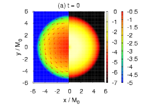
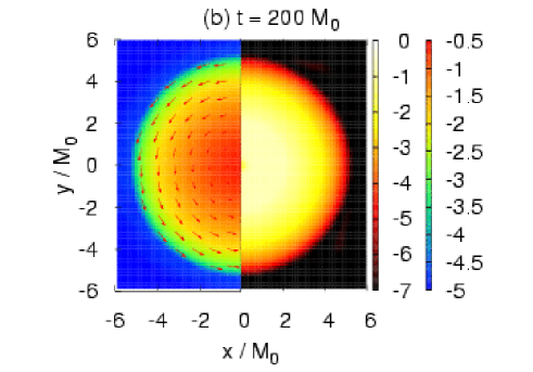
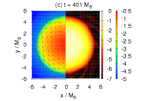
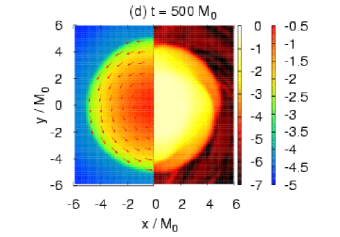
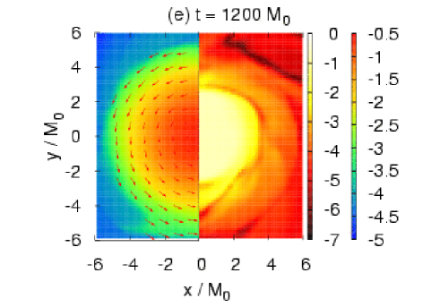
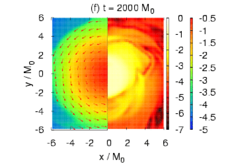
Figure 6: The same as Figure 3, but for a rotating model R22H2T8. The arrows indicate the velocity fields.

However, the instability is not suppressed by the presence of rapid rotation for all the places inside the neutron star, as Figure 2 illustrates that the central density varies for a longer-term evolution with $t\approx 2000M_{0}$. This result is totally different from that in the axisymmetric case (Kiuchi et al. 2008), in which the rapid rotation suppresses the onset of the interchange instability. Note that one of the models studied in Kiuchi et al. (2008) has similar model parameters to those of R22H08T8, which is stable for the axisymmetric perturbations. This implies that a non-axisymmetric instability is excited for the rapidly rotating models this time. To clarify the relevant instability, we generate Figures 6 and 7, in which the rest-mass density and the magnetic energy density for model R22H2T8 are plotted on the equatorial and meridian planes, respectively. Until $t\approx 200M_{0}$, we observe that the coherent magnetic field and density profiles remain. However, at $t\approx 400M_{0}$, the magnetic field profile near the stellar surface is deformed in the same manner as found for the non-rotating models. During the subsequent evolution, the coherent magnetic field structure is totally destroyed and a turbulent motion is excited. The surface expands because the plasma beta near the surface is below unity due to the leak-out of the magnetic field. Because the coherent toroidal magnetic field, which fastens the waist of the neutron star, disappears, the radius of the neutron star increases. All these features are essentially the same as for the non-rotating models.

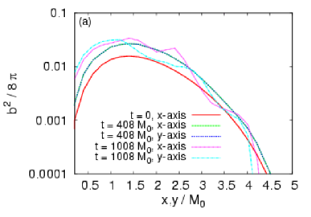
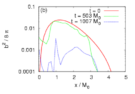
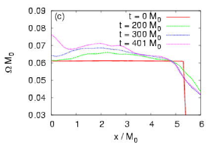
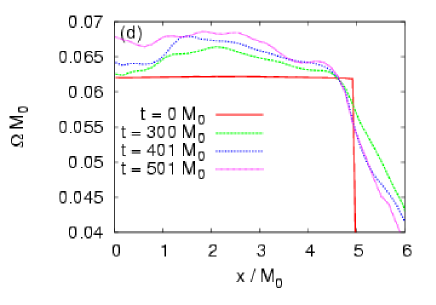
Figure 8: Snapshots of magnetic pressure (a) for model R22H2T8 and (b) for mode N22H5, and those of angular velocity profiles (c) for model R22H2T8 and (d) for model R22H08T8. Both profiles are plotted along the $x$-axis on the equator. In the panel (a), the profile along $y$-axis is also plotted. In the panels (c) and (d), it is seen that the negative gradients of the angular velocity profiles are developed near the stellar surface.

The evolution of the magnetic field near the rotation axis in the rotating models is slightly different from that in the non-rotating models. Figures 8 (a) and (b) plot the snapshots of the magnetic pressure defined by $b^{2}/8\pi$ along the $x$ and $y$-axes on the equator for models R22H2T8 and N22H5, respectively. In the rotating model R22H2T8, the profile near the center does not drastically change. However, the magnetic pressure increases gradually and systematically, and by the increased magnetic pressure, the matter near the axis is pinched. This increase proceeds in the axisymmetric way because the profiles along $y$-axis is approximately identical to those along $x$-axis in Figure 8 (a). This might seem to be incompatible with our previous results (Kiuchi et al. 2008). To clarify this point, we reconsider the criterion for the axisymmetric perturbation :

$$4\Omega^{2}\left(1+\frac{v_{A}^{2}}{c_{s}^{2}}\right)+\left(\frac{g_{\varpi}}{c_{s}^{2}}-\frac{2}{\varpi}\right)v_{A}^{2}\partial_{\varpi}\ln\left(\frac{B_{(\varphi)}}{\varpi\rho}\right)<0$$ (32)

$$g_{z}\frac{v_{A}^{2}}{c_{s}^{2}}\partial_{z}\ln\left(\frac{B_{(\varphi)}}{\varpi\rho}\right)<0$$ (33)

$$2g_{z}\varpi\Omega^{2}\frac{v_{A}^{2}}{c_{s}^{2}}\partial_{z}\ln\left(\frac{B_{(\varphi)}}{\varpi\rho}\right)<0.$$ (34)

The axisymmetric instability ignites if any of these inequalities holds. Equations  (33) and (34) implies the magnetic field profile given by Equation (22) is marginally stable. The magnetic field line strength evolves as

$$(\partial_{t}+{\rm e}^{i(a)}v_{(a)}\partial_{i})\left(\frac{B_{(\varphi)}}{\varpi\rho}\right)=\frac{{\rm e}^{i(a)}B_{(a)}}{\rho}\partial_{i}\Omega,$$ (35)

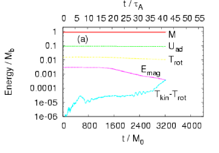
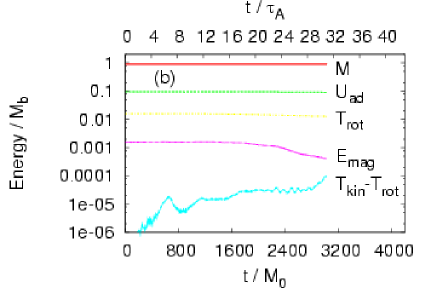
Figure 9: Time evolution of several energy components (a) for model R22H2T8 and (b) for model R22H08T8.

where ${\rm e}^{i(a)}$ is a tetrad basis. In axisymmetric simulations, the field line strength is completely preserved because the poloidal magnetic field, i.e. $B_{(\varpi)}$ and $B_{(z)}$, is never generated if the initial magnetic field is purely toroidal. Then, the inequalities (33) and (34) are never satisfied during the evolution of the magnetized star. On the other hand, the field line strength deviates from its initial value in three-dimensional simulations because the poloidal field is generated by a perturbation induced by a truncation error in general (in addition to the change of the angular velocity profile as discussed below). As the result, the inequalities (33) and (34) may hold during the evolution and the axisymmetric instability could set in. This is the reason why the magnetic pressure increases and angular velocity is distorted near the center as seen in Figures 8 (a) and (c). Note that the things are the same in model R22T08T8. It is interesting to note that the stellar surface in the rotating model expands whereas the central part contracts due to the redistribution of the magnetic field profile. Contrary to the rotating model, the coherent profile of the magnetic fields near the stellar center in the non-rotating model N22H5 disappears after the onset of the instability, which results in the systematic expansion of the star as mentioned in the previous subsection. The non-rotating models are also marginally stable against the interchange instability as shown in Equation (33). However, these models are unstable against the non-axisymmetric mode (see Figure 1 (b)) and this mode overcomes the the interchange mode. It is also interesting to note that the non-axisymmetric instability develops in an earlier time than that expected from the central density’s evolution, e.g., at $t\approx 800M_{0}(1000M_{0})$ for R22H2T8 (R22T08T8) (see Figure 2 (a)). However, the instability develops before $t\sim 600M_{0}$ for these rotating models as shown in Figure 9. This also reflects the fact that the instability, which affects the global structure of the neutron star, sets in both near the stellar surface and in the central region. Namely, the Parker (interchange) instability plays an important role in the outer (central) region for the rotating models.

The local linear perturbation analysis predicts that our rigidly rotating models are stable against the non-axisymmetric perturbation as described in Section 4.2. Thus, our numerical result does not seem to agree with that in the linear analysis. However, this is not the case, because our rotating model is close to a marginally stable state and is destabilized by a slight nonlinear perturbation to the rotational velocity. To explain this fact, we plot the snapshots of the angular velocity in Figure 8, in which the angular velocity profiles along the $x$-axis on the equator are plotted for models R22H2T8 and R22H08T8. This shows that the angular velocity deviates slightly from the constant profile and the negative gradients, in particular, near the stellar surface are developed during the evolution. This time variation is due to the oscillation of the neutron star which is initially triggered by a perturbation of numerical origin. Note that the initial conditions we gave are in equilibria, but a small numerical error associated with the finite grid resolution induces a perturbation and then the neutron stars start oscillating around their equilibrium states. Although the perturbation is induced by a numerical error in this case, it is quite natural to expect that any star in nature oscillates and thus the precisely rigid rotation is not realized. Once the angular velocity profile has the negative gradient, the instability criterion (28) could be satisfied because the first term in the left-hand side has a substantially large positive value in the rapidly rotating models with weak magnetic fields, i.e., the criterion is satisfied even for a small angular velocity gradient.

The growth process of the instability is well reflected in several energy components. Figure 9 plots their evolution. This shows that the ADM mass, adiabatic internal energy, and rotational kinetic energy remain approximately constant during the evolution. The decrease in the magnetic energy is prominent at $t\approx 1500M_{0}$ for model R22H2T8 and $t\approx 2000M_{0}$ for R22H08T8. Note that the magnetic energy increases only by $\sim 2\%$ during the development of the interchange instability, e.g, for $t\lesssim 400M_{0}$ for model R22H2T8. The kinetic energy, in which contribution of the rotational kinetic energy is excluded, increases with time. This shows that the meridian motion is developed. We find again that the rapid rotation is not enough to stabilize the instability associated with the presence of toroidal magnetic fields and the magnetic field never reaches an equilibrium state as in the non-rotating models.

It is well known that negative gradient of angular velocity in the presence of magnetic field leads to the MRI (Balbus & Hawley 1991). As discussed above, the negative angular velocity appears in the vicinity of the stellar surface. Hence, we hypothetically estimate the MRI growth rate as $\sigma_{\rm MRI}\sim\Omega\varpi|\partial_{\varpi}\ln\Omega|$. We fit the angular velocity profile as a function of the radius in Figure 8 (c-d) and obtain the gradient $\partial_{\varpi}\ln\Omega$. Putting the value of the gradient, angular velocity, and the stellar radius into the equation, we estimate the growth rate as $\sigma_{\rm MRI}M_{0}\approx 0.09$ $(0.1)$ for model R22H2T8 (R22H08T8). On the other hand, we infer the instability growth rate from the increase of the kinetic energy shown in Figure 9 with the same strategy for the non-rotating case. The resulting growth rate $\sigma M_{0}$ is $0.008$ $(0.007)$ for model R22H2T8 (R22H08T8), where we use the data of $t/M_{0}\in[0,600]$ in both the models. Therefore, the growth rates do not match. However, Equations (19) and (27) tell us that the growth rates of the interchange and Parker instability depend on the magnetic field strength. Hence, we conclude that the instability we find in the rotating model is not the MRI.

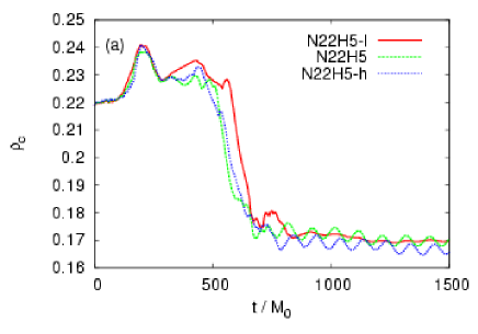
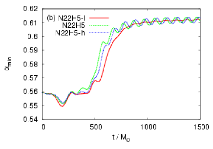
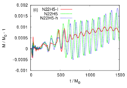
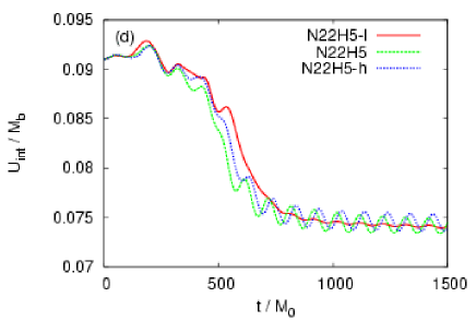
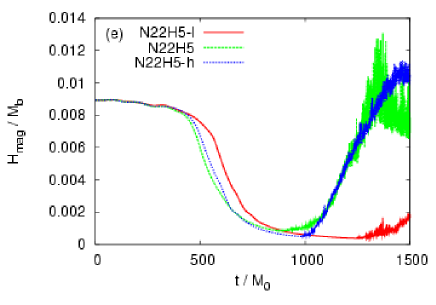
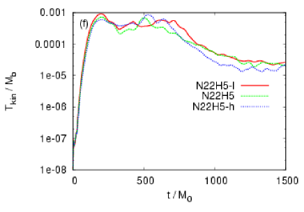
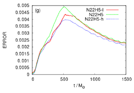
Figure 10: The results of convergence tests for model N22H5; (a) the central density, (b) the minimum value of lapse function, (c) the ADM mass normalized by its initial value, (d) the internal energy, (e) the magnetic energy, (f) the kinetic energy, and (g) the normalized Hamiltonian constraint.

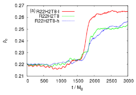
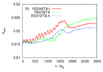
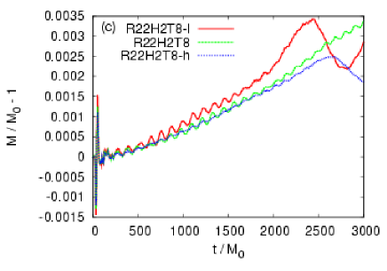
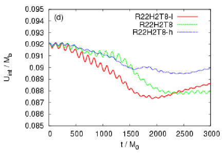
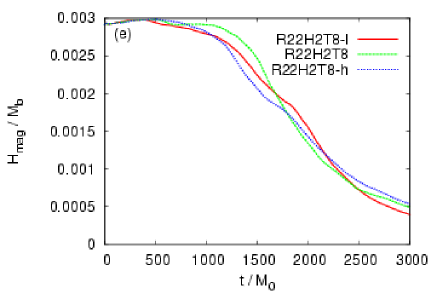
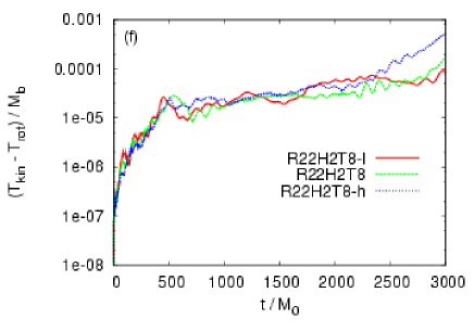
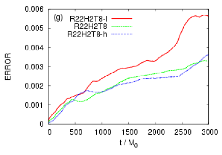
Figure 11: The same as Figure 10 but for model R22H2T8.

Before closing this section, we show that the convergence is achieved in our numerical results with an accuracy high enough to draw a quantitatively reliable conclusion. Figures 10 and 11 plot the evolution of (a) the central density, (b) the minimum value of the lapse function, (c) the ADM mass, (d) the internal energy, (e) the magnetic energy, (f) the kinetic energy, and (g) the Hamiltonian constraint violation for models N22H5 and R22H2T8. The Hamiltonian constraint violation is defined by

$${\rm ERROR}=\frac{1}{M_{b}}\int\rho w\sqrt{\gamma}|V|d^{3}x$$ (36)

with

$$V\equiv\frac{\tilde{\Delta}\psi-\frac{\psi}{8}{\tilde{R}^{k}}_{k}+2\pi\rho_{\rm H}\psi^{5}+\frac{\psi^{5}}{8}\left(\tilde{A}_{ij}\tilde{A}^{ij}-\frac{2}{3}K^{2}\right)}{|\tilde{\Delta}\psi|+|\frac{\psi}{8}{\tilde{R}^{k}}_{k}|+|2\pi\rho_{\rm H}\psi^{5}|+\frac{\psi^{5}}{8}\left(\tilde{A}_{ij}\tilde{A}^{ij}+\frac{2}{3}K^{2}\right)}$$ (37)

where $\tilde{\Delta}$ is the Laplacian associated with $\tilde{\gamma}_{ij}$, $\psi$ is the conformal factor, and $\rho_{H}=(\rho h+b^{2}/4\pi)w^{2}-(P+b^{2}/8\pi)-(\alpha b^{t})^{2}/4\pi$. In all the panels, we plot the results of three different grid resolutions. In Figure 10 (a), (b), (d), and (e), we find a transition time at $t\sim 500M_{0}$ depends slightly on the grid resolution, but on the whole, the results appear to be convergent. The ADM mass, which is approximately conserved in the present situation, is conserved within 99.8 percent accuracy (see Figure 10 (c)) and the error in the Hamiltonian constraint violation is in an acceptable level (less than $\sim 1$% error; see Figure 10 (g)). In the panel (e), we observe that the convergence is lost for $t\gtrsim 1000M_{0}$. This is likely to be caused by the turbulent field developing both outside and inside the star as shown in Figures 3 (f) and 4 (f). To handle such a region and/or turbulent field, we would need more sophisticated numerical scheme.

From these figures, we conclude that all the qualitative features of the magnetic field instability found in this work are independent of the grid resolution. In the rotating model R22H2T8, we find essentially the same features in the convergence study.

6 Summary & Discussion

6.1 Summary

We explored the non-axisymmetric instability of neutron stars with purely toroidal magnetic fields. Preparing the non-rotating and rotating neutron stars in equilibrium as the initial conditions, the three-dimensional GRMHD simulations were performed. For the non-rotating models, the local linear perturbation analysis predicts that the Parker instability would be the primary instability and we confirmed this. Due to the Parker instability, a turbulent state is developed and the initially coherent magnetic field profile is totally varied. The magnetic field profile never reaches an equilibrium state. This fact is in sharp contrast with that in the axisymmetric instability of Kiuchi et al. (2008). The growth time scale of the Parker instability depends on the magnetic field strength, i.e., the Alfvén time scale, and this result also agrees with the local linear perturbation analysis. The present result strongly suggests that three-dimensional treatment is crucial to clarify the instability of a neutron star with toroidal magnetic fields. In other words, any a priori assumption of the spacetime symmetry (e.g., axisymmetric symmetry) could prevent from deriving the correct conclusion.

We also explored the instability of rigidly and rapidly rotating neutron stars. The linear analyses have suggested that rapid rotation could play a role as a stabilizing agent. We confirm that the rapid rotation stabilizes the Tayler instability, which may occur near the axis of $\varpi=0$ in the non-rotating case. However, the interchange instability could play a minor role because the neutron stars are marginally stable against it. We note that the interchange mode never develops in the axisymmetric simulations due to the symmetry imposed. We also find that the Parker instability which is relevant near the stellar surface may not be stabilized by the rapid rotation. The reason is that by a perturbative oscillation, neutron stars may have a region in which the gradient in the angular velocity profile is negative ($\partial\Omega/\partial\varpi<0$). This negative gradient can induce the Parker instability in the case that the neutron star has rapid rotation and weak magnetic fields. As in the non-rotating model, a turbulent state is subsequently developed in the outer region of the neutron star. This result also gives us a message that the three-dimensional simulation is essential for investigating a magnetic field instability.

6.2 Discussion

As mentioned in Introduction, a large number of core-collapse supernova simulations based on the magneto-rotational mechanism have shown that toroidal magnetic fields are dominantly amplified in the proto-neutron stars via the winding mechanism. In the assumption of axial symmetry, these fields may be in quasi-equilibrium after the saturation is reached. However, this could disagree with the result in the linear perturbation analysis, i.e., the neutron stars with purely toroidal magnetic fields are often unstable. The present study indeed suggests that such neutron stars are unstable and thus the assumptions of axial symmetry and rapid rotation, which are imposed for most of the magneto-hydrodynamical supernova simulations, would be inappropriate. (Note that in axial symmetry, the rapid rotation stabilizes neutron stars with toroidal magnetic fields, as illustrated in Kiuchi et al. (2008).) In a non-axisymmetric simulation, we may find that a proto-neutron star with strongly toroidal magnetic fields is unstable and a turbulent motion inside it is excited. Magneto-hydrodynamic simulations have to be performed in fully three spatial dimensions.

Stability of more generic magnetic field configurations, i.e., mixed poloidal-toroidal fields, is quite important because such fields would be in general realized. Recently, Braithwaite & Nordlund (2005); Braithwaite & Spruit (2004); Duez et al. (2010) studied the stability of Newtonian stars with such fields, and reported that the mixed field may play an important role in stabilization; they showed that the equilibrium profile is maintained over several Alfvén time scales. We plan to study this issue with the weak magnetic field solution obtained by Ioka & Sasaki (2004) in the fully general relativistic framework.

Recently, Lander et al. (2010) and Lander & Jones (2010) studied the instability associated with the presence of toroidal magnetic fields by solving the linearized Newtonian MHD equations with their time-domain code. They showed that the Tayler instability characterized by the azimuthal mode number $m=1$ primarily occurs near the axis of $\varpi=0$ and that no pronounced Parker instability sets in near the surface of the star . Similar results were obtained by Duez et al. (2010), in which Newtonian resistive MHD simulations are performed. These results seem to be incompatible with our present results. The reason for this discrepancy seems to be the following: Lander et al. (2010) and Lander & Jones (2010) restrict their studies to low-order azimuthal modes ($m\leq 6$) and Duez et al. (2010) employs some kinds of (artificial) viscosity and resistivity for the evolution to remove numerical instability caused by a short-wavelength oscillation. Note that Lander et al. (2010) and Lander & Jones (2010) also use artificial viscosity to stabilize their computations. This suggests that in their simulations, short-wavelength modes might be suppressed. As can be seen from Figures 1 and 3, the Parker instability found in this study is characterized by a high-order azimuthal mode number, which implies that the unstable modes of the Parker instability near the surface have a short wavelength. In Duez et al. (2010), they used a stably stratified model with the polytrope index $n=3$ and forecasted the instability as we did in Figure 1. They found the primarily instability is not the Parker instability, but the Taylor instability in their model. This is likely that the restoring force due to the entropy gradient near the surface stabilizes the magnetic buoyant force.

Finally, we comment on a possible potential effect for stabilizing the magnetic field instabilities which are not taken into account in our present work. In a stably stratified region of the star, the buoyant force inhibits the interchange, Parker, and Tayler instabilities from growing (Acheson 1978). For the cold neutron star, the composition gradient induced by chemical inhomogeneities can stably stratify the neutron star matter and supports the gravity mode (g-mode) oscillations. Finn (1987) considered crustal g-modes due to the composition discontinuities in the outer envelopes, whose typical oscillation period is about 5 ms for a canonical neutron star model. Reisenegger & Goldreich (1992) studied the effect of g-modes associated with buoyancy induced by proton-neuron composition gradients in the core, whose typical oscillation period is about 2 ms for a canonical neutron star model. If the growth time scale of the Parker instability found in our study is longer than these periods of the g-modes, it is possible that the buoyant forces inside the neutron star suppress the growth of the Parker instability. In the present study, we find that a typical growth time scale of the Parker instability is about $20M_{0}$, which gives a typical growth time scale of 0.1 ms for a canonical neutron star model with a strong magnetic field of $10^{16}$ G. For the present models, thus, it seems that the buoyancy inside the neutron star could not suppress the onset of the Parker instability. However, for a weaker magnetic field strength $\approx 10^{15}$ G, the Parker instability could be suppressed by the buoyancy because a typical growth time scale of the Parker instability becomes 1 ms. To derive a definite answer to this problem, whether or not the buoyancy can stabilize the Parker instability inside the neutron star, we have to know the local growth rate of the Parker instability. Unfortunately, in our simulations, it is difficult to estimate it in the vicinity of the stellar surface because the local magnetic structure highly depends on the numerical resolution. To investigate this point more precisely, we have to take into account the chemical inhomogeneities; this implies that it is necessary to implement equations of state which depend on the chemical compositions and to obtain the evolution of the chemical compositions. This is beyond the scope of this paper.

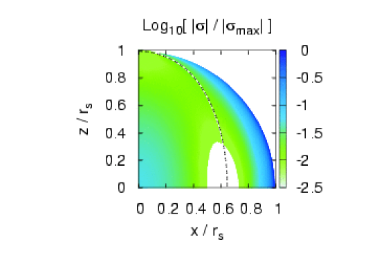
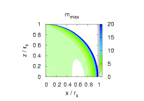
Figure 1: The growth rate of the instability of a neutron star with toroidal magnetic fields normalized by the maximum growth rate $|\sigma_{\rm max}|$ (left) and corresponding $m$ mode (right) on the meridian plane for non-rotating Newtonian polytrope with $\rho_{0}=0.16$ and $B_{0}=0.2$. The white colored region and the dotted curve denote the stable region and critical radius, respectively. $r_{s}$ denotes the stellar radius.

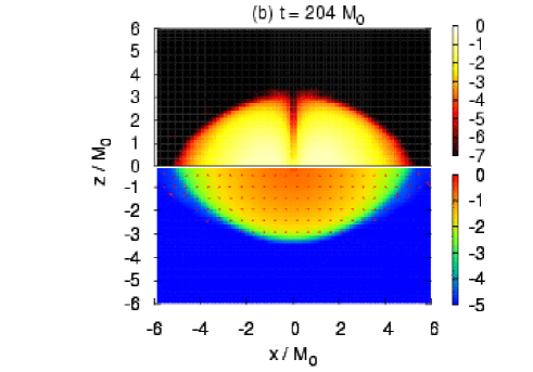
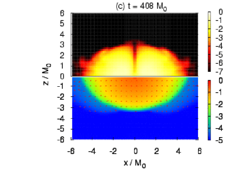
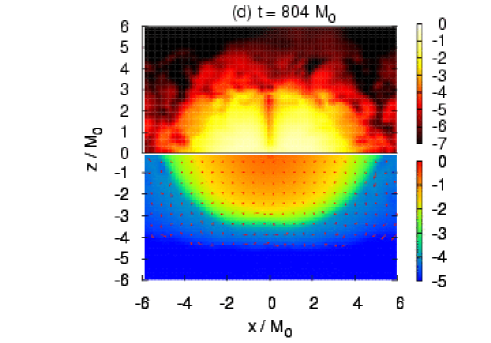
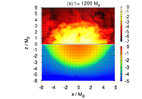
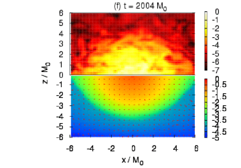
Figure 7: The same as Figure 4, but for a rotating model R22H2T8.

References

- Acheson (1978) Acheson, D. J., 1978, Phil. Trans. Roy. Soc. Lond. A, 289, 459
- Baker et al. (2006) Baker, J. G., Centrella, J., Choi, D.-I., Koppitz, M., and van Meter, J., 2006, Phys. Rev. Lett. 96, 111102
- Balbus & Hawley (1991) Balbus, S. A., and Hawley, J. F., 1991, Astrophys. J. ,376, 214
- Baumgarte & Shapiro (1999) Baumgarte, T. W., and Shapiro, S. L., 1999, Phys. Rev. D 59, 024007
- Bildsten et al. (1997) Bildsten, L. et al.,1997, Astrophys. J. Suppl., 113, 367
- Braithwaite & Nordlund (2005) Braithwaite, J. and Nordlund, A., 2005, Astron. Astrophys. 450, 1077
- Braithwaite & Spruit (2004) Braithwaite, J., and Spruit, H. C., 2004, Nature, 431, 819
- Burrows et al. (2007) Burrows, A., Dessart, L., Livne, E., Ott, C. D., and Murphy, J., 2007, Astrophys. J. 664, 416
- Brugmann et al. (2008) Brugmann, B., Gonzalez, J. A., Hannam, M., Husa, S., Sperhake, U., and Tichy, W., 2008, Phys. Rev. D 77, 024027
- Campanelli et al. (2006) Campanelli, M., Lousto, C. O., Marronetti, P., and Zlochower, Y., 2006, Phys. Rev. Lett. 96, 111101
- Cook et al. (1994) Cook, G. B., Shapiro, S. L., and Teukolsky, S. A. 1994, Astrophys. J. 422, 227
- Duez et al. (2010) Duez, V., Braithwaite, J., Mathis, S., arXiv:1009.5384 [astro-ph.SR]
- Finn (1987) Finn, L. S., 1987, Mon. Not. R. Astro. Soc., 227, 265
- Goossens (1980) Goossens, M., 1980, Geo. Astro. Fluid. Dyn., 15, 123
- Gavriil et al. (2002) Gavriil, F. P., Kaspi, V., M., and Woods, P. M., 2002, Nature, 419, 142
- Harding & Lai (2006) Harding, A. K., and Lai, D., 2006, Rept. Prog. Phys. 69, 2631
- Ibrahim et al. (2003) Ibrahim, A. I., Swank, J. H., Parke, W., 2003, Astrophys. J. , 584, L17
- Ioka & Sasaki (2004) Ioka, K. and Sasaki, M. 2004, Astrophys. J. 600, 296
- Kotake et al. (2004) Kotake, K., Sawai, H., Yamada, S., and Sato, K., 2004, Astrophys. J. , 608, 391
- Kiuchi et al. (2009) Kiuchi, K., Sekiguchi, Y., Shibata, M., and Taniguchi, K., 2009, Phys. Rev. D 80, 064037
- Kiuchi et al. (2008) Kiuchi, K., Shibata, M., and Yoshida, S., 2008, Phys. Rev. D 78, 024029
- Kiuchi & Yoshida (2008) Kiuchi, K., and Yoshida, S., 2008, Phys. Rev. D 78, 044045
- Kurganov & Tadmor (2000) Kurganov, A., and Tadmor, E., 2000, J. Comput. Phys. 160, 214
- Lai (2001) Lai, D., 2001 Rev. Mod. Phys., 73, 629
- Lander et al. (2010) Lander, S. K., Jones D. I., and Passamonti, A., 2010, Mon. Not. R. Astro. Soc., 405, 318
- Lander & Jones (2010) Lander, S. K., and Jones D. I., arXiv:1009.2453
- Lucas-Serrano et al. (2004) Lucas-Serrano, A., Font, J. A., Ibánez, J. M. and Martí, J. M., 2004, Astron. Astrophys. 428, 703
- Manchester et al. (2005) Manchester, R. N., Hobbs, G. B., Teoh, A., and Hobbs, M., 2005, AJ, 129, 1993: see http://www.atnf.csiro.au/research/pulsar/psrcat/ for the latest number of pulsars
- Obergaulinger et al. (2006) Obergaulinger, M., Aloy, M.A., and Müller, 2006, Astron. Astrophys. 450, 1107
- Orlandini & Fiume (2001) Orlandini, M. and Fiume, D. D., 2001, AIP Conference Proceedings, 599, 283,
- Cerda-Duran et al. (2007) Cerda-Duran, P., Font, J. A., and Dimmelmeier, H., 2007, Astron. Astrophys. 474, 169
- Parker (1955) Parker, E. N., 1955, ApJ, 121, 49
- Parker (1966) Parker, E. N., 1966, ApJ, 145, 811
- Reisenegger & Goldreich (1992) Reisenegger, A., and Goldreich, P., 1992, Astrophys. J. 395, 240
- Rea et al. (2003) Rea, N. et al., 2003, Astrophys. J. 586, L65
- Scheidegger et al. (2008) Scheidegger, S., Fischer, T., and Liebendoerfer, M., 2008, Astron. Astrophys., 490, 231
- Shibata (2003) Shibata, M., 2003, Phys. Rev. D 67, 024033
- Shibata & Nakamura (1995) Shibata, M. and Nakamura, T., 1995, Phys. Rev. D 52, 5428
- Shibata & Sekiguchi (2005) Shibata, M. and Sekiguchi, Y. i., 2005, Phys. Rev. D 72, 044014
- Shibata et al. (2006) Shibata, M., Liu, Y., T., Shapiro, S. L., and Stephens, B. C., 2006, Phys. Rev. D 74, 104026
- Spruit (1999) Spruit, H. C., 1999, Astron. Astrophys., 349, 189
- Takiwaki et al. (2009) Takiwaki, T., Kotake, K., and Sato, K., 2009, Astrophys. J. 691, 1360
- Tayler (1973) Tayler, R. J., 1973, Mon. Not. R. Astro. Soc., 161, 365
- Thompson & Duncan (1993) Thompson, C., and Duncan, R. C., 1993, Astrophys. J. 408, 194
- Thompson & Duncan (1995) Thompson, C., and Duncan, R. C., 1995, Mon. Not. R. Astro. Soc., 275, 255
- Thompson & Duncan (1996) Thompson, C., and Duncan, R. C., 1996, Astrophys. J. 473, 322
- Thompson & Duncan (2001) Thompson, C., and Duncan, R. C., 2001, Astrophys. J. , 561, 980
- Wickramasinghe & Ferrario (2005) Wickramasinghe, D., and Ferrario, L. 2005, Mon. Not. Roy. Astron. Soc. 356, 1576
- Woods & Thompson (2004) Woods, P. M., and Thompson, C., arXiv:astro-ph/0406133.
- Yamada & Sawai (2004) Yamada, S., & Sawai, H., 2004, Astrophys. J. , 608, 907