Optimal coding for the deletion channel
with small deletion probability

Abstract

The deletion channel is the simplest point-to-point communication channel that models lack of synchronization. Input bits are deleted independently with probability $d$, and when they are not deleted, they are not affected by the channel. Despite significant effort, little is known about the capacity of this channel, and even less about optimal coding schemes. In this paper we develop a new systematic approach to this problem, by demonstrating that capacity can be computed in a series expansion for small deletion probability. We compute three leading terms of this expansion, and find an input distribution that achieves capacity up to this order. This constitutes the first optimal coding result for the deletion channel.

The key idea employed is the following: We understand perfectly the deletion channel with deletion probability $d=0$. It has capacity 1 and the optimal input distribution is i.i.d. Bernoulli$(1/2)$. It is natural to expect that the channel with small deletion probabilities has a capacity that varies smoothly with $d$, and that the optimal input distribution is obtained by smoothly perturbing the i.i.d. Bernoulli$(1/2)$ process. Our results show that this is indeed the case. We think that this general strategy can be useful in a number of capacity calculations.

1 Introduction

The (binary) deletion channel accepts bits as inputs, and deletes each transmitted bit independently with probability $d$. Computing or providing systematic approximations to its capacity is one of the outstanding problems in information theory [1]. An important motivation comes from the need to understand synchronization errors and optimal ways to cope with them.

In this paper we suggest a new approach. We demonstrate that capacity can be computed in a series expansion for small deletion probability, by computing the first two orders of such an expansion. Our main result is the following.

Theorem 1.1.

Let $C(d)$ be the capacity of the deletion channel with deletion probability $d$. Then, for small $d$ and any ${\epsilon}>0$,

$$C(d)=1+d\log d-A_{1}\,d+A_{2}\,d^{2}+O(d^{3-\epsilon})\,,$$ (1)

where

$$A_{1} \equiv\log(2e)-\sum_{l=1}^{\infty}2^{-l-1}l\log l\approx 1.15416377$$

$$A_{2} =c_{3}+c_{4}+\frac{1}{4\ln 2}\left(2+\frac{3}{2}c_{2}^{2}+\sum_{l=1}^{\infty}2^{-l}\left(l\ln l\right)^{2}-c_{2}\sum_{l=1}^{\infty}2^{-l}l^{2}\ln l\right)\approx 1.67814594$$

$$c_{2} \equiv\sum_{l=1}^{\infty}2^{-l}l\ln l\approx 1.78628364$$

$$c_{3} \equiv\frac{1}{2}\left(-1+\sum_{l=3}^{\infty}2^{-l}\left\{\binom{l}{2}\log\binom{l}{2}-l^{2}\log l+(l-1)(l-3)\log(l-1)+(l-2)\log(l-2)\right\}\,\right)$$

$$\approx\,-0.88636960$$

$$c_{4} \equiv\sum_{j=4}^{\infty}2^{-(2+j)}\,(j-1)(j-3)\,h\!\left(\frac{1}{j-1}\right)$$

$$\phantom{\equiv\ }+\sum_{i=2}^{\infty}\sum_{j=4}^{\infty}2^{-(i+j+1)}\,(i+j-1)(j-3)\,h\!\left(\frac{i+1}{i+j-1}\right)\approx 0.69001321$$

Here $h(\cdot)$ is the binary entropy function, i.e., $h(p)\equiv-p\log p-(1-p)\log(1-p)$.

Further, the binary stationary source defined by the property that the times at which it switches from $0$ to $1$ or viceversa form a renewal process with holding time distribution $p_{L}(l)=2^{-l}(1+d(l\ln l-c_{2}l/2))$, achieves rate within $O(d^{3-\epsilon})$ of capacity.

Given a binary sequence, we will call ‘runs’ its maximal blocks of contiguous $0$’s or $1$’s. We shall refer to binary sources such that the switch times form a renewal process as sources (or processes) with i.i.d. runs.

The ‘rate’ of a given binary source is the maximum rate at which information can be transmitted through the deletion channel using input sequences distributed as the source. A formal definition is provided below (see Definition 2.3). Logarithms denoted by $\log$ here (and in the rest of the paper) are understood to be in base $2$. While one might be skeptical about the concrete meaning of asymptotic expansions of the type (1), they often prove surprisingly accurate. For instance at $d=0.1$ ($10\%$ of the input symbols are deleted), the expression in Eq. (1) (dropping the error term $O(d^{3-{\epsilon}})$) is larger than the best lower bound [2] by about $0.007$ bits. The lower bound of [2] is derived using a Markov source and ‘jigsaw’ decoding. Our asymptotic analysis implies that the loss in rate due to restricting to Markov sources and jigsaw decoding (cf. Theorem 6.1 and Remark 6.2), to leading order, is $0.904d^{2}\approx 0.009$. Hence, we estimate that our asymptotic approach incurs an error of about $0.002$ bits for computing the capacity at $d=0.1$.

More importantly asymptotic expansions can provide useful design insight. Theorem 1.1 shows that the stationary process consisting of i.i.d. runs with the specified run length distribution, achieves capacity to within $O(d^{3-\epsilon})$. In comparison, the best performing approach tried before this was to use a first order Markov source for coding [2]. We are able to show, in fact, that this approach incurs a loss that is $\Omega(d^{2})$, which is the same order as the loss incurred by the trivial approach of using i.i.d. Bernoulli$(1/2)$!

Remark 1.2.

In this work, we prove rigorous upper and lower bounds on capacity that match up to quadratic order in $d$ (cf. Theorem 1.1), but without explicitly evaluating the constants in the error terms. It would be very interesting to obtain explicit expressions for these constants.

Before this work, there was no non-trivial optimal coding result known for the deletion channel. Further terms in the capacity expansion can be expected to supply even more detailed information about the optimal coding scheme and allow us to achieve capacity to higher orders.

We think that the strategy adopted here might be useful in other information theory problems. The underlying philosophy is that whenever capacity is known for a specific value of the channel parameter, and the corresponding optimal input distribution is unique and well characterized, it should be possible to compute an asymptotic expansion around that value. In the present context the special channel is the perfect channel, i.e. the deletion channel with deletion probability $d=0$. The corresponding input distribution is the i.i.d. Bernoulli$(1/2)$ process.

1.1 Related work

Dobrushin [3] proved a coding theorem for the deletion channel, and other channels with synchronization errors. He showed that the maximum rate of reliable communication is given by the maximal mutual information per bit, and proved that this can be achieved through a random coding scheme. This characterization has so far found limited use in proving concrete estimates. An important exception is provided by the work of Kirsch and Drinea [4] who use Dobrushin coding theorem to prove lower bounds on the capacity of channels with deletions and duplications. We will also use Dobrushin theorem in a crucial way, although most of our effort will be devoted to proving upper bounds on the capacity.

Several capacity bounds have been developed over the last few years, following alternative approaches, and are surveyed in [1]. In particular, it has been proved that $C(d)=\Theta(1-d)$ as $d\to 1$ [5]. The papers [6, 7] improve the upper bound in this limit obtaining $\limsup_{d\to 1}C(d)/(1-d)\leq 0.413$. However, determining the asymptotic behavior in this limit (i.e. finding a constant $B_{1}$ such that $C(d)=B_{1}(1-d)+o(1-d)$) is an open problem. When applied to the small $d$ regime, none of the known upper bounds actually captures the correct behavior as stated in Eq. (1). A simple calculation shows that the first upper bound in [8] has asymptotics of $1+(3/4)d\log d$. Another work [6] shows that $C\geq 1-4.19d$ as $d\rightarrow\infty$. As we show in the present paper, this behavior can be controlled exactly, up to the third leading term of the expansion.

A short version of this paper was presented at the 2010 International Symposium on Information Theory (ISIT) [9]. At the same conference, Kalai, Mitzenmacher and Sudan [10] presented a result analogous to Theorem 1.1. The proof is based on a counting argument, very different from the the techniques employed here. Also, the result of [10] is not the same as in Theorem 1.1, since only the $d\log d$ term of the series is established in [10]. Theorem 1.1 improves on our ISIT result [9], that contained only the first two terms in the series expansion, but not the order $d^{2}$ term. Also, we obtain a non-trivial coding scheme for the first time in this paper. The trivial i.i.d. Bernoulli$(1/2)$ coding scheme is enough to achieve capacity up to linear order as shown in our conference paper [9].

1.2 Numerical illustration of results

We can numerically evaluate the expression in Eq. (1) (dropping the error term) to obtain estimates of capacity for small deletion probabilities.

$$C_{\textup{\tiny est}}=1+d\log d-A_{1}\,d+A_{2}\,d^{2}\,.$$

The values of $C_{\textup{\tiny est}}$ are presented in Table 1 and Figure 1. We compare with the best known numerical lower bounds [2] and upper bounds [6, 8].

We stress here that $C_{\textup{\tiny est}}$ is neither an upper nor a lower bound on capacity. It is an estimate based on taking the leading terms of the asymptotic expansion of capacity for small $d$, and is expected to be accurate for small values of $d$. Indeed, we see that for $d$ larger than $0.4$, our estimate $C_{\textup{\tiny est}}$ exceeds the upper bound. This simply indicates that we should not use $C_{\textup{\tiny est}}$ as an estimate for such large $d$. We believe that $C_{\textup{\tiny est}}$ provides an excellent estimate of capacity for $d\apprle 0.2$.

$d$	Best lower bound	$C_{\textup{\tiny est}}$	Best upper bound
0.05	0.7283	0.7304	0.8160
0.10	0.5620	0.5692	0.6890
0.15	0.4392	0.4541	0.5790
0.20	0.3467	0.3719	0.4910
0.25	0.2759	0.3163	0.4200
0.30	0.2224	0.2837	0.3620
0.35	0.1810	0.2715	0.3150
0.40	0.1484	0.2781	0.2750
0.45	0.1229	0.3020	0.2410
0.50	0.1019	0.3425	0.2120

Table 1: Table showing best known numerical bounds on capacity (from [2, 6, 8]) compared with our estimate based on the small $d$ expansion.

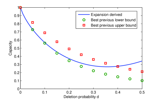
Figure 1: Plot showing best known numerical bounds on capacity (from [2, 6, 8]) compared with our estimate based on the small $d$ expansion.

1.3 Notation

We borrow $O(\cdot)$, $\Omega(\cdot)$ and $\Theta(\cdot)$ notation from the computer science literature. We define these as follows to fit our needs. Let $f:[0,1]\rightarrow\mathbb{R}$ and $g:[0,1]\rightarrow\mathbb{R_{+}}$. We say:

• We say $f=O(g)$ if there is a constant $c<\infty$ such that $|f(x)|\leq cg(x)$ for all $x\in[0,1]$.

• We say $f=\Omega(g)$ if there is a constant $c>0$ such that $f(x)\geq cg(x)$ for all $x\in[0,1]$.

• We say $f=\Theta(g)$ if there are constants $c<\infty\,,\,c^{\prime}>0$ such that $cg(x)\geq f(x)\geq c^{\prime}g(x)$ for all $x\in[0,1]$.

Throughout this paper, we adhere to the convention that the constants $c,c^{\prime}$ above should not depend on the processes $\mathbb{X},\mathbb{Y},\ldots$ etc. under consideration, if there are such processes.

1.4 Outline of the paper

Section 2 contains the basic definitions and results necessary for our approach to estimating the capacity of the deletion channel. We show that it is sufficient to consider stationary ergodic input sources, and define their corresponding rate (mutual information per bit). Capacity is obtained by maximizing this quantity over stationary processes. In Section 3, we present an informal argument that contains the basic intuition leading to our main result (Theorem 1.1), and allows us to correctly guess the optimal input distribution. Section 4 states a small number of core lemmas, and shows that they imply Theorem 1.1. Finally, Section 5 states several technical results (proved in appendices) and uses them to prove the core lemmas. We conclude with a short discussion, including a list of open problems, in Section 6.

2 Preliminaries

For the reader’s convenience, we restate here some known results that we will use extensively, along with some definitions and auxiliary lemmas.

Consider a sequence of channels $\{W_{n}\}_{n\geq 1}$, where $W_{n}$ allows exactly $n$ inputs bits, and deletes each bit independently with probability $d$. The output of $W_{n}$ for input $X^{n}$ is a binary vector denoted by $Y(X^{n})$. The length of $Y(X^{n})$ is a binomial random variable. We want to find maximum rate at which we can send information over this sequence of channels with vanishingly small error probability.

The following characterization follows from [3].

Theorem 2.1.

Let

$$C_{n}\equiv\frac{1}{n}\max_{p_{X^{n}}}\,I(X^{n};Y(X^{n}))\,.$$

Then, the following limit exists

$$C\equiv\lim_{n\rightarrow\infty}C_{n}=\inf_{n\geq 1}C_{n}\,,$$ (2)

and is equal to the capacity of the deletion channel.

A further useful remark is that, in computing capacity, we can assume $(X_{1},\dots,X_{n})$ to be $n$ consecutive coordinates of a stationary ergodic process. We denote by $\mathcal{S}$ the class of stationary and ergodic processes that take binary values.

Lemma 2.2.

Let $\mathbb{X}=\{X_{i}\}_{i\in{\mathbb{Z}}}$ be a stationary and ergodic process, with $X_{i}$ taking values in $\{0,1\}$. Then the limit $I(\mathbb{X})=\lim_{n\rightarrow\infty}\frac{1}{n}I(X^{n};Y(X^{n}))$ exists and

$$C=\max_{\mathbb{X}\in\mathcal{S}}I(\mathbb{X})\,.$$

We use the following natural definition of the rate achieved by a stationary ergodic process.

Definition 2.3.

For stationary and ergodic $\mathbb{X}$, we call $I(\mathbb{X})=\lim_{n\rightarrow\infty}\frac{1}{n}I(X^{n};Y(X^{n}))$ the rate achieved by $\mathbb{X}$.

Proofs of Theorem 2.1 and Lemma 2.2 are provided in Appendix A.

Given a stationary process $\mathbb{X}$, it is convenient to consider it from the point of view of a ‘uniformly random’ block/run. Intuitively, this corresponds to choosing a large integer $n$ and selecting as reference point the beginning of a uniformly random block in $X_{1},\dots,X_{n}$. Notice that this approach naturally discounts longer blocks for finite $n$. While such a procedure can be made rigorous by taking the limit $n\rightarrow\infty$, it is more convenient to make use of the notion of Palm measure from the theory of point processes [11, 12], which is, in this case, particularly easy to define. To a binary source $\mathbb{X}$, we can associate in a bijective way a subset of times ${\mathbb{S}}\subseteq\mathbb{Z}$, by letting $t\in{\mathbb{S}}$ if and only if $X_{t}$ is the first bit of a run. The Palm measure $\mathbb{P}_{1}$ is then the distribution of $\mathbb{X}$ conditional on the event $1\in{\mathbb{S}}$.

We denote by $L$ the length of the block starting at $1$ under the Palm measure, and denote by $p_{L}$ its distribution. As an example, if $\mathbb{X}$ is the i.i.d. Bernoulli$(1/2)$ process, we have $p_{L}=p_{L}^{*}$ where $p_{L}^{*}(l)\equiv 2^{-l}$. We will also call $p_{L}$ the block-perspective run length distribution or simply the run length distribution, and let

$$\mu(\mathbb{X})\equiv\mathbb{E}\sum_{l=1}^{\infty}p_{L}(l)\,l\,,$$

be its average. Let $L_{0}$ be the length of the block containing bit $X_{0}$ in the stationary process $\mathbb{X}$. A standard calculation[11, 12] yields $\mathbb{P}(L_{0}=l)=lp_{L}(l)/\mu(\mathbb{X})\,$. Since $L_{0}$ is a well defined and almost surely finite (by ergodicity), we necessarily have $\mu(\mathbb{X})<\infty$.

In our main result, Theorem 1.1, a special role is played by processes $\mathbb{X}$ such that the associated switch times form a stationary renewal process. We will refer to such an $\mathbb{X}$ as a process with i.i.d. runs.

3 Intuition behind the main theorem

In this section, we provide a heuristic/non-rigorous explanation for our main result. The aim is build intuition and motivate our approach, without getting bogged down with the numerous technical difficulties that arise. In fact, we focus here on heuristically deriving the optimal input process $\mathbb{X}^{\dagger}$, and do not actually obtain the quadratic term of the capacity expansion. We find $\mathbb{X}^{\dagger}$ by computing various quantities to leading order and using the following observation (cf. Remark 4.2).

Key Observation: The process that achieves capacity for small $d$ should be ‘close’ to the Bernoulli$(1/2)$ process, since $H(\mathbb{X})$ must be close to $1$.

We have

$$I(X^{n};Y(X^{n}))=H(Y)-H(Y|X^{n})\,.$$ (3)

Let $D^{n}$ be a binary vector containing a one at position $i$ if and only if $X_{i}$ is deleted from the input vector. We can write

$$H(Y|X^{n})=H(Y,D^{n}|X^{n})-H(D^{n}|X^{n},Y)\,.$$

But $Y$ is a function of $(X^{n},D^{n})$, leading to $H(Y,D^{n}|X^{n})=H(D^{n}|X^{n})=H(D^{n})=nh(d)$, where we used the fact that $D^{n}$ is i.i.d. Bernoulli($d$), independent of $X^{n}$. It follows that

$$H(Y|X^{n})=nh(d)-H(D^{n}|X^{n},Y)\,.$$ (4)

The term $H(D^{n}|X^{n},Y)$ represents ambiguity in the location of deletions, given the input and output strings. Now, since $d$ is small, we expect that most deletions occur in ‘isolation’, i.e., far away from other deletions. Make the (incorrect) assumption that all deletions occur such that no three consecutive runs have more than one deletion in total. In this case, we can unambiguously associate runs in $\mathbb{Y}$ with runs in $\mathbb{X}$. Ambiguity in the location of a deletion occurs if and only if a deletion occurs in a run of length $l>1$. In this case, each of $l$ locations is equally likely for the deletion, leading to a contribution of $\log l$ to $H(D^{n}|X^{n},Y)$. Now, a run of length $l$ should suffer a deletion with probability $\approx ld$. Thus, we expect

$$\frac{1}{n}\,H(D^{n}|X^{n},Y)\approx\frac{d}{\mu(\mathbb{X})}\sum_{l=1}^{\infty}p_{L}(l)l\log l\,.$$

We know that $H(\mathbb{X})$ is close to $1$, implying $\mu(\mathbb{X})$ is close to $2$ and $p_{L}$ is close to $p_{L}^{*}(l)\equiv 2^{-l}$. This leads to

$$\frac{1}{n}\,H(D^{n}|X^{n},Y) \approx\frac{d}{2}\sum_{l=1}^{\infty}p_{L}(l)l\log l+\frac{d(\mu(\mathbb{X})-2)}{4}\sum_{l=1}^{\infty}p_{L}^{*}(l)l\log l$$

$$=\frac{d}{2}\left[-\frac{c_{2}}{\ln 2}+\sum_{l=1}^{\infty}p_{L}(l)l\left(\log l-\frac{c_{2}}{2\ln 2}\right)\right]\,.$$ (5)

Consider $H(Y)$. Now, if the input $X^{n}$ is drawn from a stationary process $\mathbb{X}$, we expect the output $Y(X^{n})$ to also be a segment of some stationary process $\mathbb{Y}$. (It turns out that this is the case.) Moreover, we expect that the channel output has $n(1-d)+o(n)$ bits, leading to $H(Y)\approx n(1-d)H(\mathbb{Y})$. Denote the run length distribution in $\mathbb{Y}$ by $q_{L}(\cdot)$. Define $\mu(\mathbb{Y})\equiv\sum_{l=1}^{\infty}q_{L}(l)l$. Let $L_{\mathbb{Y}}$ denote the length of a random run drawn according to $q_{L}(\cdot)$. It is not hard to see that

$$H(\mathbb{Y})\leq H(L_{\mathbb{Y}})/\mu(\mathbb{Y})\,,$$

with equality iff $\mathbb{Y}$ consists of i.i.d. runs, which occurs iff $\mathbb{X}$ consists of i.i.d. runs. Define $q_{L}^{*}(l)\equiv 2^{-l}$. An explicit calculation yields $H(L_{\mathbb{Y}})=1-D(q_{L}||q_{L}^{*})/\mu(\mathbb{Y})$. We know that $H(\mathbb{Y})$ is close to $1$, implying $\mu(\mathbb{Y})$ is close to $2$ and $D(q_{L}||q_{L}^{*})$ is small. Thus,

$$\lim_{n\rightarrow\infty}\frac{1}{n}\,H(Y)=(1-d)H(\mathbb{Y})\leq(1-d)(1-D(q_{L}||q_{L}^{*})/\mu(\mathbb{Y}))\approx 1-d-D(q_{L}||q_{L}^{*})/2\,.$$

Notice that an i.i.d. Bernoulli$(1/2)$ input results in an i.i.d. Bernoulli$(1/2)$ output from the deletion channel. The following is made precise in Lemma 5.9: Let $\Delta$ be the ‘distance’ between $p_{L}$ and $p_{L}^{*}$. Then a short calculation tells us that the distance between $p_{L}$ and $q_{L}$ should be $O(d^{1-{\epsilon}}\Delta)$. In other words $p_{L}$ and $q_{L}$ are very nearly equal to each other.

So we obtain, to leading order,

$$\lim_{n\rightarrow\infty}\frac{1}{n}\,H(Y)\apprle 1-d-D(p_{L}||p_{L}^{*})/2\,,$$ (6)

with (approximate) equality iff $\mathbb{X}$ consists of i.i.d. runs.

Putting Eqs. (3), (4), (5) and (6) together, we have

$$I(\mathbb{X}) =\lim_{n\rightarrow\infty}\frac{1}{n}I(X^{n};Y)$$

$$\apprle 1-d-D(p_{L}||p_{L}^{*})/2-h(d)+\frac{d}{2}\left[-\frac{c_{2}}{\ln 2}+\sum_{l=1}^{\infty}p_{L}(l)l\left(\log l-\frac{c_{2}}{2\ln 2}\right)\right]$$

$$\approx 1-d\log(1/d)-A_{1}d-\frac{1}{2}D(p_{L}||p_{L}^{*})+\frac{d}{2}\left[\sum_{l=1}^{\infty}p_{L}(l)l\left(\log l-\frac{c_{2}}{2\ln 2}\right)\right]\,.$$

Since this (approximate) upper bound on $I(\mathbb{X})$ depends on input $\mathbb{X}$ only through $p_{L}$, we choose $\mathbb{X}$ consisting of i.i.d. runs so that (approximate) equality holds.

We expect $p_{L}$ to be close to $p_{L}^{*}(l)$. A Taylor expansion gives

$$D(p_{L}||p_{L}^{*}) =\sum_{l=1}^{\infty}p_{L}(l)(l+\log p_{L}(l))$$

$$\approx\frac{1}{\ln 2}\sum_{l=1}^{\infty}\bigg{(}\left(p_{L}(l)-2^{-l}\right)+2^{l-1}\left(p_{L}(l)-2^{-l}\right)^{2}\bigg{)}$$

$$=\frac{1}{\ln 2}\sum_{l=1}^{\infty}2^{l-1}\left(p_{L}(l)-2^{-l}\right)^{2}\,.$$

Thus, we want to maximize

$$\frac{1}{2\ln 2}\sum_{l=1}^{\infty}2^{l-1}\left(p_{L}(l)-2^{-l}\right)^{2}+\frac{d}{2}\left[\sum_{l=1}^{\infty}p_{L}(l)l\left(\log l-\frac{c_{2}}{2\ln 2}\right)\right]\,,$$

subject to $\sum_{l=1}^{\infty}p_{L}(l)=1$, in order to achieve the largest possible $I(\mathbb{X})$. A simple calculation tells us that the maximizing distribution is $p_{L}^{\dagger}(l)=2^{-l}(1+d(l\ln l-c_{2}l/2))$.

4 Proof of the main theorem: Outline

In this section we provide the proof of Theorem 1.1 after stating the key lemmas involved. We defer the proof of the lemmas to the next section. Sections 5.1-5.4 develop the technical machinery we use, and the proofs of the lemmas are in Section 5.6.

Given a (possibly infinite) binary sequence, a run of $0$’s (of $1$’s) is a maximal subsequence of consecutive $0$’s ($1$’s), i.e. an subsequence of $0$’s bordered by $1$’s (respectively, of $1$’s bordered by $0$’s). The first step consists in proving achievability by estimating $I(\mathbb{X})$ for a process having i.i.d. runs with appropriately chosen distribution.

Lemma 4.1.

Let $\mathbb{X}^{\dagger}$ be the process consisting of i.i.d. runs with distribution $p_{L}^{\dagger}(l)=2^{-l}(1+d(l\log l-c_{2}l/2))$. Then for any ${\epsilon}>0$, we have

$$I(\mathbb{X}^{\dagger})=1+d\log d-A_{1}\,d+A_{2}\,d^{2}+O(d^{3-{\epsilon}})\,.$$

Lemma 4.1 is proved in Section 5.6.

Lemma 2.2 allows us to restrict our attention to stationary ergodic processes in proving the converse. For a process $\mathbb{X}$, we denote by $H(\mathbb{X})$ its entropy rate. Define

$$H(Y_{\mathbb{X}})\equiv\lim_{n\rightarrow\infty}\frac{H(Y(X^{n}))}{n(1-d)}\,.$$ (7)

A simple argument shows that this limit exists and is bounded above by $1$ for any stationary process $\mathbb{X}$ and any $d$, with $H(Y_{\mathbb{X}})=1$ iff $\mathbb{X}$ is the i.i.d. Bernoulli($1/2$) process.

In light of Lemma 4.1, we can restrict consideration to processes $\mathbb{X}$ satisfying $I(\mathbb{X})>1-d^{1-\epsilon}$ whence $H(\mathbb{X})>1-d^{1-\epsilon},H(Y_{\mathbb{X}})>1-d^{1-\epsilon}$:

Remark 4.2.

There exists $d_{0}({\epsilon})>0$ such that for all $d<d_{0}({\epsilon})$, if $I(\mathbb{X})>C-d$, we have $I(\mathbb{X})>1-d^{1-\epsilon}$ and hence also $H(\mathbb{X})>1-d^{1-\epsilon}\,,\ H(Y_{\mathbb{X}})>1-d^{1-\epsilon}$ .

We define a ‘super-run’ next.

Definition 4.3.

A super-run consists of a maximal contiguous sequence of runs such that all runs in the sequence after the first one (on the left) have length one. We divide a realization of $\mathbb{X}$ into super-runs $\ldots,S_{-1},S_{0},S_{1},\ldots\,$. Here $S_{1}$ is the super-run including the bit at position 1.

See Table 2 for an example showing division into super-runs.

$\ldots$	$b_{-4}$	$b_{-3}$	$b_{-2}$	$b_{-1}$	$b_{0}$	$b_{1}$	$b_{2}$	$b_{3}$	$b_{4}$	$b_{5}$	$b_{6}$	$b_{7}$	$b_{8}$	$\ldots$
$\ldots$	1	0	0	1	0	0	0	1	1	0	1	0	0	$\ldots$

Table 2: An example showing how $\mathbb{X}$ is divided into super-runs

Denote by $\mathcal{S}$ the set of all stationary ergodic processes and by $\mathcal{S}_{L^{*}}$ the set of stationary ergodic processes such that, with probability one, no super-run has length larger than $L^{*}$.

Our next lemma tightens the constraint given by Remark 4.2 further for processes in $\mathcal{S}_{\lfloor 1/d\rfloor}$.

Lemma 4.4.

Consider any $\epsilon>0$ and constant $\kappa$. There exists $d_{0}(\epsilon,\kappa)>0$ such that the following happens for any $\mathbb{X}\in\mathcal{S}_{\lfloor 1/d\rfloor}$. For any $d<d_{0}$, if

$$I(\mathbb{X}) \geq C-\kappa d^{2-(\epsilon/2)}\,,$$

then

$$H(Y_{\mathbb{X}})\geq 1-d^{2-\epsilon}\,.$$

We show an upper bound for the restricted class of processes $\mathcal{S}_{L^{*}}$.

Lemma 4.5.

For any ${\epsilon}>0$ there exists $d_{0}=d_{0}({\epsilon})>0$ and $\kappa<\infty$ such that the following happens. If $d<d_{0}(\epsilon)$, for any $\mathbb{X}\in\mathcal{S}_{\lfloor 1/d\rfloor}$,

$$I(\mathbb{X})\leq 1+d\log d-A_{1}d+A_{2}d^{2}+\kappa d^{3-\epsilon}\,.$$

Finally, we show a suitable reduction from the class $\mathcal{S}$ to the class $\mathcal{S}_{L^{*}}$.

Lemma 4.6.

For any ${\epsilon}>0$ there exists $d_{0}=d_{0}({\epsilon})>0$ such that the following happens for all $d<d_{0}$, and all $\gamma>0$. For any $\mathbb{X}\in\mathcal{S}$ such that $H(Y_{\mathbb{X}})>1-d^{\gamma}$ and for any $L^{*}>2\gamma\log(1/d)$, there exists $\mathbb{X}_{L^{*}}\in\mathcal{S}_{L^{*}}$ such that

$$I(\mathbb{X}) \leq I(\mathbb{X}_{L^{*}})+d^{\gamma-\epsilon}(L^{*})^{-1}\log L^{*}\,,$$ (8)

$$H(Y_{\mathbb{X}}) \geq H(Y_{\mathbb{X}_{L^{*}}})-d^{\gamma-\epsilon}(L^{*})^{-1}\log L^{*}\,.$$ (9)

Lemmas 4.4, 4.5 and 4.6 are proved in Section 5.6.

The proof of Theorem 1.1 follows from these lemmas with Lemma 4.6 being used twice.

Proof of Theorem 1.1.

Lemma 4.1 shows achievability. For the converse, we start with a process $\mathbb{X}\in\mathcal{S}$ such that $I(\mathbb{X})>C-d^{3}$. By Remark 4.2, $H(Y_{\mathbb{X}})>1-d^{1-\delta}$ for any $\delta>0$ and $d<d_{0}(\delta)$. Use Lemma 4.6, with $\gamma=1-\delta$, $L^{*}=\lfloor 1/d\rfloor$ and ${\epsilon}=\delta/2$. It follows that for $d<d_{0}(\delta/2)$,

$$I(\mathbb{X}_{L^{*}}) >C-d^{2-2\delta}\,,$$

$$H(Y_{\mathbb{X}}) \geq H(Y_{\mathbb{X}_{L^{*}}})-d^{2-2\delta}\,.$$

We now use Lemma 4.4 which yields $H(Y_{\mathbb{X}_{L^{*}}})\geq 1-d^{2-2\delta}$ and hence, by Eq. (9), $H(Y_{\mathbb{X}})\geq 1-2d^{2-2\delta}\geq 1-d^{2-3\delta}$ for small $d$. Now, we can use Lemma 4.6 again with $\gamma=2-3\delta$, $L^{*}=\lfloor 1/d\rfloor$, ${\epsilon}=\delta/2$. We obtain

$$I(\mathbb{X}_{L^{*}})\geq C-d^{3-4\delta}\,.$$

Finally, using Lemma 4.5, we get the required upper bound on $C$. ∎

5 Proofs of the Lemmas

In Section 5.1 we show that, for any stationary ergodic $\mathbb{X}$ that achieves a rate close to capacity, the run-length distribution must be close to the distributions obtained for the i.i.d. Bernoulli$(1/2)$ process. In Section 5.2, we suitably rewrite the rate $I(\mathbb{X})$ achieved by stationary ergodic process $\mathbb{X}$ as the sum of three terms. In Section 5.3 we construct a modified deletion process that allows accurate estimation of $H(Y|X^{n})$ in the small $d$ limit. Section 5.4 proves a key bound on $H(Y_{\mathbb{X}})$ that leads directly to Lemma 4.4. Finally, in Section 5.6 we present proofs of the Lemmas quoted in Section 4 using the tools developed.

We will often write $X_{a}^{b}$ for the random vector $(X_{a},X_{a+1},\dots,X_{b})$ where the $X_{i}$’s are distributed according to the process $\mathbb{X}$.

5.1 Characterization in terms of runs

Let $m_{n}$ be the number of runs in $X^{n}$. Let $L_{1}^{+},L_{2},\dots,L_{m_{n}}$ be the run lengths ($L_{1}^{+}$ being the length of the intersection of that run with $X^{n}$). It is clear that $H(X^{n})\leq 1+H(m_{n},L_{1}^{+},L_{2},\dots,L_{m_{n}})$ (where one bit is needed to remove the $0,1$ ambiguity). By ergodicity $m_{n}/n\to 1/\mathbb{E}[L]$ almost surely as $n\to\infty$. Also $m_{n}\leq n$ implies $H(m_{n})/n\leq\log n/n\to 0$. Further, $\limsup_{n\rightarrow\infty}H(L_{1}^{+},L_{2},\dots,L_{m_{n}})/n\leq\lim_{n\rightarrow\infty}H(L)m_{n}/n=H(L)/\mathbb{E}[L]$. If $H(\mathbb{X})$ is the entropy rate of the process $\mathbb{X}$, by taking the $n\to\infty$ limit, it is easy to deduce that

$$H(\mathbb{X})\leq\frac{H(L)}{\mathbb{E}[L]}\,,$$ (10)

with equality if and only if $\mathbb{X}$ is a process with i.i.d. runs with common distribution $p_{L}$.

We know that given $\mathbb{E}[L]=\mu$, the probability distribution with largest possible entropy $H(L)$ is geometric with mean $\mu$, i.e. $p_{L}(l)=(1-1/\mu)^{l-1}1/\mu$ for all $l\geq 1$, leading to

$$\frac{H(L)}{\mathbb{E}[L]}\leq-\big{(}1-\frac{1}{\mu}\big{)}\log\big{(}1-\frac{1}{\mu}\big{)}-\frac{1}{\mu}\log\frac{1}{\mu}\equiv h(1/\mu)\,.$$ (11)

Here we introduced the notation $h(p)=-p\log p-(1-p)\log(1-p)$ for the binary entropy function.

Using this, we are able to obtain sharp bounds on $p_{L}$ and $\mu(\mathbb{X})$.

Lemma 5.1.

There exists $d_{0}>0$ such that the following occurs. For any $\beta>1/2$ and $d<d_{0}$, if $\mathbb{X}\in\mathcal{S}$ is such that $H(\mathbb{X})>1-d^{\beta}$, we have

$$|\mu(\mathbb{X})-2|\leq 7\,d^{\beta/2}\,.$$ (12)

Proof.

By Eqs. (10) and (11), we have $h(1/\mu)\geq 1-d^{\beta}$. By Pinsker’s inequality $h(p)\leq 1-(1-2p)^{2}/(2\ln 2)$, and therefore $|1-(2/\mu)|^{2}\leq(2\ln 2)d^{\beta}$. The claim follows from simple calculus. ∎

Lemma 5.2.

There exists $d_{0}>0$ and $\kappa^{\prime}<\infty$ such that the following occurs for any $\beta>1/2$ and $d<d_{0}$. For any $\mathbb{X}\in\mathcal{S}$ such that $H(\mathbb{X})>1-d^{\beta}$, we have

$$\sum_{l=1}^{\infty}\left|p_{L}(l)-\frac{1}{2^{l}}\right|\leq\kappa^{\prime}d^{\beta/2}\,.$$ (13)

Proof.

Let $p_{L}^{*}(l)=1/2^{l},\ l\geq 1$ and recall that $\mu(\mathbb{X})=\mathbb{E}[L]=\sum_{l\geq 1}p_{L}(l)l$. An explicit calculation yields

$$H(L)=\mu(\mathbb{X})-D(p_{L}||p_{L}^{*})\,.$$ (14)

Now, by Pinsker’s inequality,

$$D(p_{L}||p_{L}^{*})\geq\frac{2}{\ln 2}\lVert p_{L}-p_{L}^{*}\rVert_{\rm TV}^{2}\,.$$ (15)

Combining Lemma 5.1, and Eqs. (10), (14) and (15), we get the desired result. ∎

For the rest of Section 5.1, we only state our technical estimates, deferring proofs to Appendix B.

We now state a tighter bound on probabilities of large run lengths. We will find this useful, for instance, to control the number of bit flips in going from general $\mathbb{X}$ to $\mathbb{X}_{L^{*}}$ having bounded run lengths.

Lemma 5.3.

There exists $d_{0}>0$ such that the following occurs: Consider any $\beta>1/2$, and define $\ell\equiv\lfloor 2\beta\log(1/d)\rfloor$. For all $d<d_{0}$, if $\mathbb{X}\in\mathcal{S}$ is such that $H(\mathbb{X})>1-d^{\beta}$, we have

$$\sum_{l=\ell}^{\infty}\ lp_{L}(l)\ \leq 20d^{\beta}\,,$$ (16)

We use $L(k)$ to denote the vector of lengths $(L_{1},L_{2},\ldots,L_{k})$ of a randomly selected block of $k$ consecutive runs (a ‘$k$-block’). Formally, $(L_{1},L_{2},\dots,L_{k})$ is the vector of lengths of the first $k$ runs starting from bit $X_{1}$, under the Palm measure $\mathbb{P}_{1}$ introduced in Section 2.

Corollary 5.4.

There exists $d_{0}>0$ such that the following occurs: Consider any positive integer $k$ and any $\beta>1/2$, and define $\ell\equiv\lfloor 2\beta\log(1/d)\rfloor$. For all $d<d_{0}$, if $\mathbb{X}\in\mathcal{S}$ is such that $H(\mathbb{X})>1-d^{\beta}$, we have

$$\sum_{l_{1}+\ldots+l_{k}\geq k\ell}\,(l_{1}+\ldots+l_{k})p_{L(k)}(l_{1},\ldots,l_{k})\ \leq 20k^{2}d^{\beta}\,.$$ (17)

Clearly, $\mathbb{E}[L_{1}+\ldots+L_{k}]=k\mu(\mathbb{X})$. We have

$$H(\mathbb{X})\leq\frac{H(L_{1},L_{2},\ldots,L_{k})}{k\mu(\mathbb{X})}\,.$$

A stronger form of Lemma 5.2 follows.

Lemma 5.5.

Let $p_{L(k)}^{*}(l_{1},\dots,l_{k})\equiv 2^{-\sum_{i=1}^{k}l_{i}}$. For the same $\kappa^{\prime}$ and $d_{0}>0$ as in Lemma 5.2, the following occurs. Consider any positive integer $k$ and any $\beta>1/2$. For all $d<d_{0}$, if $\mathbb{X}\in\mathcal{S}$ is such that $H(\mathbb{X})>1-d^{\beta}$, we have

$$\sum_{l_{1}=1}^{\infty}\sum_{l_{2}=1}^{\infty}\ldots\sum_{l_{k}=1}^{\infty}\left|p_{L(k)}(l_{1},\ldots,l_{k})-p_{L(k)}^{*}(l_{1},\ldots,l_{k})\right|\leq\kappa^{\prime}\sqrt{k}\,d^{\beta/2}\,.$$

We now relate the run-length distribution in $\mathbb{X}$ and in $Y(X^{n})$ (as $n\rightarrow\infty$). For this, we first need a characterization of $Y$ in terms of a stationary ergodic process. Let $\mathbb{D}=(\ldots,D_{-1},D_{0},D_{1},D_{2},\ldots)$ be an i.i.d. Bernoulli$(d)$, independent of $\mathbb{X}$. Construct $\mathbb{Y}$ as follows. Look at $X_{1},X_{2},\ldots$. Delete bits corresponding to $D_{1},D_{2},\ldots$. The bits remaining are $Y_{1},Y_{2},\ldots$ in order. Similarly, in $X_{0},X_{-1},X_{-2},\ldots$ delete bits corresponding to $D_{0},D_{-1},D_{-2},\ldots$. The bits remaining are $Y_{0},Y_{-1},\ldots$ in order.

Proposition 5.6.

The process $\mathbb{Y}$ is stationary and ergodic for any stationary ergodic $\mathbb{X}$.

Notice on the other hand that $(\mathbb{X},\mathbb{Y})$ are not jointly stationary.

The channel output $Y(X^{n})$ is then $(\mathbb{Y})_{1}^{M}$ where $M\sim\textup{Binomial}(n,1-d)$. It is easy to check that

$$H(\mathbb{Y})=H(Y_{\mathbb{X}})$$

(cf. Eq. (7)). We will henceforth use $H(\mathbb{Y})$ instead of the more cumbersome notation $H(Y_{\mathbb{X}})$.

Let $q_{L}$ denote the block perspective run-length distribution for $\mathbb{Y}$. Denote by $q_{L(k)}$ the block perspective distribution for $k$-blocks in $\mathbb{Y}$. Lemmas 5.1, 5.2, 5.3, 5.5 and Corollary 5.4 hold for any stationary ergodic process, hence they hold true if we replace $(\mathbb{X},p)$ with $(\mathbb{Y},q)$.

In proving the upper bound, it turns out that we are able to establish a bound of $H(\mathbb{Y})>1-d^{2-{\epsilon}}$ for ${\epsilon}>0$ and small $d$, but no corresponding bound for $H(\mathbb{X})$. Next, we establish that if $H(\mathbb{Y})$ is close to $1$, this leads to tight control over the tail for $p_{L}(\,\cdot\,)$. This is a corollary of Lemma 5.3.

Lemma 5.7.

There exists $d_{0}>0$ such that the following occurs: Consider any $\gamma>1/2$, and define $\ell\equiv\lfloor 2\gamma\log(1/d)\rfloor$. For all $d<d_{0}$, if $H(\mathbb{Y})\geq 1-d^{\gamma}$, we have

$$\sum_{l=2\ell}^{\infty}\ lp_{L}(l)\ \leq 80d^{\gamma}\,.$$

Note that $p_{L}$ refers to the block length distribution of $\mathbb{X}$, not $\mathbb{Y}$.

Corollary 5.8.

There exists $d_{0}>0$ such that the following occurs: Consider any positive integer $k$ and $\gamma>1/2$, and define $\ell\equiv\lfloor 2\gamma\log(1/d)\rfloor$. For all $d<d_{0}$, if $H(\mathbb{Y})\geq 1-d^{\gamma}$, we have

$$\sum_{l=2kl_{0}}^{\infty}\ (l_{1}+\ldots+l_{k})p_{L(k)}(l_{1},\ldots,l_{k})\ \leq 80k^{2}d^{\gamma}\,.$$

Consider $\mathbb{X}$ being i.i.d. Bernoulli$(1/2)$. Clearly, this corresponds to $\mathbb{Y}$ also i.i.d. Bernoulli$(1/2)$. Hence, each has the same run length distribution $p_{L}^{*}(l)=q_{L}^{*}(l)=2^{-l}$. This happens irrespective of the deletion probability $d$. Now suppose $\mathbb{X}$ is not i.i.d. Bernoulli$(1/2)$ but approximately so, in the sense that $H(\mathbb{X})$ close to $1$. The next lemma establishes, that in this case also, the run length distribution of $\mathbb{Y}$ is very close to that of $\mathbb{X}$, for small run lengths and small $d$.

Lemma 5.9.

There exist a function $(\kappa,{\epsilon})\mapsto d_{0}(\kappa,{\epsilon})>0$ and constants $\kappa_{1}<\infty$, $\kappa_{2}<\infty$ such that the following happens, for any $\beta\in(1/2,2)$, ${\epsilon}>0$ and $\kappa<\infty$.
(i) For all $d<d_{0}$, for all $\mathbb{X}$ such that $H(\mathbb{X})>1-d^{\beta}$, and all $l<\kappa\log(1/d)$, we have

$$|p_{L}(l)-q_{L}(l)|\leq\kappa_{1}d^{1+\beta/2-{\epsilon}}\,.$$

(ii) For all $d<d_{0}$ and all $\mathbb{X}$ such that $H(\mathbb{X})>1-d^{\beta}$, we have

$$|\mu(\mathbb{X})-\mu(\mathbb{Y})|\leq\kappa_{2}d^{1+\beta/2}\,.$$ (18)

Let us emphasize that $\kappa_{1},\kappa_{2}$ do not depend at all on $\beta,{\epsilon},\kappa$, where as $d_{0}$ does not depend on $\beta$ in the above lemma. Analogous comments apply to the remaining lemmas in this section.

As before, we are able to generalize this result to blocks of $k$ consecutive runs.

Lemma 5.10.

There exist a function $(\kappa,{\epsilon})\mapsto d_{0}(\kappa,{\epsilon})>0$ and a constant $\kappa<\infty$ such that the following happens, for any $\beta\in(1/2,2)$, ${\epsilon}>0$ and $\kappa<\infty$.

For all $d<d_{0}$, for all integers $k>0$ and $(l_{1},l_{2},\ldots,l_{k})$ such that $\sum_{i=1}^{k}l_{i}<\kappa\log(1/d)$, and all $\mathbb{X}$ such that $H(\mathbb{X})>1-d^{\beta}$, we have

$$|p_{L(k)}(l_{1},\ldots,l_{k})-q_{L(k)}(l_{1},\ldots,l_{k})|\leq\kappa^{\prime}\,d^{1+\beta/2-{\epsilon}}\,.$$

In proving the lower bound, we have $H(\mathbb{X}^{\dagger})=1-O(d^{2})$, but no corresponding bound for $H(\mathbb{Y})$. The next lemma allows us to get tight control over the tail of $q_{L}^{\dagger}(\cdot)$.

Lemma 5.11.

For any ${\epsilon}>0$, there exists $d_{0}\equiv d_{0}({\epsilon})>0$ such that the following occurs: Consider any $\beta\in(1/2,2]$, and define $\ell\equiv\lfloor 4\log(1/d)\rfloor$. For all $d<d_{0}$, if $H(\mathbb{X})\geq 1-d^{\beta}$, we have

$$\sum_{l=\ell}^{\infty}\ lq_{L}(l)\ \leq d^{\beta-{\epsilon}}\,.$$

Define $p_{L(k)}^{*}(l_{1},\ldots,l_{k})\equiv 2^{-\sum_{i=1}^{k}l_{i}}$. We show, using Lemma 5.10, that if $H(\mathbb{Y})$ is close to 1, than one can bound the distance between $p_{L(k)}(\,\cdot\,)$ and $p_{L(k)}^{*}(\,\cdot\,)$.

Lemma 5.12.

There exist a function $(\kappa,{\epsilon})\mapsto d_{0}(\kappa,{\epsilon})>0$ and constants $\kappa_{1}<\infty$, $\kappa_{2}<\infty$ such that the following happens, for any ${\epsilon}>0$ and $\kappa<\infty$.
(i) For all $d<d_{0}$, all sources $\mathbb{X}$ such that $H(\mathbb{X})>1-d^{0.6}$ and $H(\mathbb{Y})>1-d^{\gamma}$, and all integers $k>0$ and $(l_{1},l_{2},\ldots,l_{k})$ such that $\sum_{i=1}^{k}l_{i}<\kappa\log(1/d)$, we have

$$|p_{L(k)}(l_{1},\ldots,l_{k})-p_{L(k)}^{*}(l_{1},\ldots,l_{k})| \leq\,d^{\gamma/2-{\epsilon}}\,,$$ (19)

$$|p_{L(k)}(l_{1},\ldots,l_{k})-q_{L(k)}(l_{1},\ldots,l_{k})| \leq\,d^{1+\gamma/2-{\epsilon}}\,.$$ (20)

(ii) For all $d<d_{0}$, all sources $\mathbb{X}$ such that $H(\mathbb{X})>1-d^{0.6}$ and $H(\mathbb{Y})>1-d^{\gamma}$, we have

$$|\mu(\mathbb{X})-2| \leq\kappa_{1}d^{\gamma/2}\,,$$ (21)

$$|\mu(\mathbb{X})-\mu(\mathbb{Y})| \leq\kappa_{2}d^{1+\gamma/2}\,.$$ (22)

The next Lemma assures us that if $\mathbb{X}\in\mathcal{S}_{\lfloor 1/d\rfloor}$, then very few runs in $\mathbb{Y}$ are much longer than ${\lfloor 1/d\rfloor}$. In fact, we show that $q_{L}(\lambda{\lfloor 1/d\rfloor})$ decays exponentially in $\lambda$.

Lemma 5.13.

There exists $d_{0}>0$ such that, for all $d<d_{0}$, the following occurs: Consider any $\mathbb{X}\in\mathcal{S}_{\lfloor 1/d\rfloor}$ such that $H(\mathbb{X})>1-d^{2/3}$. Then, for all $\lambda>2$ such that $\lambda\lfloor 1/d\rfloor$ is an integer, we have

$$q_{L}(\lambda\lfloor 1/d\rfloor)\leq d^{\lambda-2}\,.$$

Next, we prove some analogous results for super-runs, cf. Definition 4.3, that we also need.

We denote by $\widetilde{L}^{\textup{\tiny rep}}$ the length of the first run in a random super-run and by $\widetilde{L}^{\textup{\tiny alt}}$ the total length of the remaining runs of the same super-run. More precisely, we repeat here the construction of Section 2, and define a new Palm measure, $\mathbb{P}_{s1}$, which is the measure of $\mathbb{X}$ conditional on $X_{1}$ being the first bit of a super-run. Then, $\widetilde{L}^{\textup{\tiny rep}}$ the length of the first run of this super-run, and $\widetilde{L}^{\textup{\tiny alt}}$ is the residual length of the same super run, always under the Palm measure $\mathbb{P}_{s1}$. Here ‘rep’ indicates ‘repeated’ with $\widetilde{L}^{\textup{\tiny rep}}$ being the number of repeated bits and ‘alt’ indicates ‘alternating’ with $\widetilde{L}^{\textup{\tiny alt}}$ being the number of alternating bits. We denote the type of a random super run by $\widetilde{T}\equiv(\widetilde{L}^{\textup{\tiny rep}},\widetilde{L}^{\textup{\tiny alt}})$ and the length by $\widetilde{L}\equiv\widetilde{L}^{\textup{\tiny alt}}+\widetilde{L}^{\textup{\tiny rep}}$. We need versions of Lemmas 5.3 and 5.7 for super-runs.

Define $\widetilde{\mu}(\mathbb{X})\equiv 1/\mathbb{E}[\widetilde{L}]$. It is easy to see that

$$H(\mathbb{X})\leq\frac{H(\widetilde{T})}{\widetilde{\mu}(\mathbb{X})}\,.$$ (23)

We denote by $p_{\widetilde{T}}$ the distribution of $\widetilde{T}$. Define $p_{\widetilde{T}}^{*}(l_{1},l_{2})\equiv 2^{-l_{1}-l_{2}}$, this being the distribution for the i.i.d. Bernoulli$(1/2)$ process $\mathbb{X}^{*}$. We denote by $p_{\widetilde{L}}$ the distribution of $\widetilde{L}$ in $\mathbb{X}$. Clearly,

$$p_{\widetilde{L}}(l)=\sum_{l^{\textup{\tiny rep}}=2}^{l}p_{\widetilde{T}}(l^{\textup{\tiny rep}},l-l^{\textup{\tiny rep}})\,.$$

Lemma 5.14.

There exists $d_{0}>0$ such that the following occurs. For any $\beta>1/2$ and $d<d_{0}$, if $\mathbb{X}\in\mathcal{S}$ is such that $H(\mathbb{X})>1-d^{\beta}$, we have

$$|\widetilde{\mu}(\mathbb{X})-4|\leq 4\,d^{\beta/2}\,.$$

Lemma 5.15.

There exists $d_{0}>0$ such that the following occurs: Consider any $\beta>1/2$, and define $\ell\equiv\lfloor 2\beta\log(1/d)\rfloor$. For all $d<d_{0}$, if $\mathbb{X}\in\mathcal{S}$ is such that $H(\mathbb{X})>1-d^{\beta}$, we have

$$\sum_{l=\ell}^{\infty}lp_{\widetilde{L}}(l)\leq 40d^{\beta}\,.$$

Let $q_{\widetilde{L}}(\cdot)$ the distribution of super-run lengths in $\mathbb{Y}$, and $\widetilde{\mu}(\mathbb{Y})$ denote the mean length of a super-run in $\mathbb{Y}$.

Lemma 5.16.

There exists $d_{0}>0$ such that the following occurs: Consider any $\gamma>1/2$, and define $\ell\equiv\lfloor 2\gamma\log(1/d)\rfloor$. For all $d<d_{0}$, if $H(\mathbb{X})\geq 1-d^{0.6}$ and $H(\mathbb{Y})\geq 1-d^{\gamma}$, we have

$$\sum_{l=\ell}^{\infty}\ lp_{\widetilde{L}}(l)\ \leq 80d^{\gamma}\,.$$

Note that $p_{\widetilde{L}}$ refers to the super-run length distribution of $\mathbb{X}$, not $\mathbb{Y}$.

Corollary 5.17.

There exists $d_{0}>0$ such that the following occurs: Consider any positive integer $k$, any $\gamma>1/2$, and define $\ell\equiv\lfloor 2\gamma\log(1/d)\rfloor$. For all $d<d_{0}$, if $H(\mathbb{X})\geq 1-d^{0.6}$ and $H(\mathbb{Y})\geq 1-d^{\gamma}$, we have

$$\sum_{l_{1}+\ldots+l_{k}\geq k\ell}^{\infty}\ (l_{1}+\ldots+l_{k})p_{\widetilde{L}(k)}(l_{1},\ldots,l_{k})\ \leq 80k^{2}d^{\gamma}\,.$$

Proofs of all results stated in Section 5.1 above (except the first two) are available in Appendix B.

5.2 Rate achieved by a process

We make use of an approach similar to that of Kirsch and Drinea [4] to evaluate $I(\mathbb{X})$ for a stationary ergodic process $\mathbb{X}$ that may be used to generate an input for the deletion channel. A fundamental difference is that [4] only considers processes with i.i.d. runs. Our analysis is instead general. This enables us to obtain tight upper and lower bounds (up to $O(d^{3-{\epsilon}})$), hence leading to an estimate for the channel capacity.

We depart from the notation of Kirsch and Drinea, retaining $X_{i}$ for the $i$th bit of $X$, and using $Y(j)$ to denote the $j$th run in $Y(X^{n})$. Denote by $L_{1},L_{2},\ldots,L_{m}$ the lengths of runs in $X_{1}^{n}$ (where $m$ is a non-decreasing function of $n$ for any fixed $X_{1}^{\infty}$). Let the $i$th run consists of $b(i)$’s, where $b(i)\in\{0,1\}$. For instance, if the first run consists of $0$’s, then $b(i)=i+1\;(\textup{mod }2)$.

We use $X(j)$ to denote the concatenation of runs in $X$ that led to $Y(j)$, with the first run in $X(j)$ contributing at least one bit (if the run is completely deleted, then it is part of $X(j-1)\,$). $X(1)$ is an exception. This is made precise in Table 3, which is essentially the same as [4, Figure 1], barring changes in notation. We call runs in $X(j)$ the parent runs of the run $Y(j)$.

1:	Set $X(1)=Y(1)=$the empty string.
2:	$j\leftarrow 1$
3:	For $i=1$ to $m$ do
4:	$\sigma\leftarrow b(i)^{L_{i}}$
5:	$\omega\leftarrow$ the bits in $Y$ that arise from $i$th run in $X$
6:	% $\sigma$ is a (possibly empty) string of all $b(i)$’s.
7:	% $Y(j)$ is a (possibly empty) string of all $b(j)$’s.
8:	If $b(i)=b(j)$ or $|\omega|=0$ then
9:	% $\omega$ is contained in the current block $Y(j)$ of $Y$
10:	$Y(j)\leftarrow Y(j)\omega$
11:	$X(j)\leftarrow X(j)\sigma$
12:	Else % $\omega$ is a prefix of $Y(j+1)$
13:	$j\leftarrow j+1$
14:	$Y(j)\leftarrow Y(j)\omega$
15:	$X(j)\leftarrow X(j)\sigma$
16:	End If
17:	End For

Table 3: Procedure for generating $Y(1),Y(2),\ldots,Y(M)$ and $X(1),X(2),\ldots,X(M)$ given $X^{n}$ and $Y(X^{n})$ (adapted from [4, Figure 1]).

We define $K(X^{n})$ as the vector of $|X(j)|$. Let the total number of runs in $Y(X^{n})$ be $M$. Thus,

$$Y(X^{n})=\, Y(1)\ldots Y(M-1)Y(M)\,,$$

$$X^{n}=\, X(1)\ldots X(M-1)X(M)\,,$$

$$K(X^{n})=\, \left(|X(1)|,\ldots,|X(M-1)|\right)\,.$$

Note that $X(j)$ consists of an odd number of runs for $1<j<M$.

We write

$$I(X^{n};Y(X^{n}))=H(Y)-H(Y,K|X^{n})+H(K|X^{n},Y)\,,$$ (24)

which is analogous to the identity $I(X^{n};Y(X^{n}))=H(X^{n})-H(X^{n},K|Y)+H(K|X^{n},Y)$ used in [4], but more convenient for our proof.

Let $L_{\mathbb{Y}}$ be an integer random variable having the distribution $q_{L}$, i.e. the distribution of run length in $\mathbb{Y}$. It is easy to see that

$$\lim_{n\rightarrow\infty}\frac{H(Y(X^{n}))}{n(1-d)}=H(\mathbb{Y})\leq\frac{H(L_{\mathbb{Y}})}{\mu(\mathbb{Y})}$$

holds, similar to (10). It turns out that this suffices for our upper bound (cf. Lemma 4.4).

Consider the second term in Eq. (24). Let $D^{n}$ denote the $n$-bit binary vector that indicates which bit locations in $X^{n}$ have suffered deletions. We have

$$H(Y,K|X^{n}) =H(D^{n}|X^{n})-H(D^{n}|X^{n},Y,K)$$

$$=nh(d)-H(D^{n}|X^{n},Y,K)\,.$$ (25)

We study $H(D^{n}|X^{n},Y,K)$ by constructing an appropriate modified deletion process in Section 5.3

Consider the third term in Eq.(24). From [4], we know that

$$\lim_{n\rightarrow\infty}\frac{H(K|X^{n},Y)}{n}=\frac{\lim_{n\rightarrow\infty}H(\,|X(2)|\ |X(2)\ldots X(M),Y(2)\ldots Y(M))}{\mathbb{E}[|X(2)|]}\,.$$

Here $X(2)\ldots X(M)$ denotes the string obtained by concatenating $X(2)$, …, $X(M)$, without separation marks, and analogously for $Y(2)\ldots Y(M)$. Roughly, single deletions do not lead to ambiguity in $|X(2)|$ if $X(2)\ldots$ and $Y(2)\ldots$ are known. Thus, this term is $O(d^{2})$. It turns out we can we can get a good estimate for this term by computing it for the i.i.d. Bernoulli($1/2$) case.

Lemma 5.18.

For any ${\epsilon}>0$, there exists $d_{0}\equiv d_{0}({\epsilon})>0$, and $\kappa<\infty$ such that for all $d<d_{0}$ the following occurs: Consider any $\mathbb{X}\in\mathcal{S}_{\lfloor 1/d\rfloor}$ such that $H(\mathbb{X})>1-d^{1-{\epsilon}}$ and $\max\{H(\mathbb{X}),H(\mathbb{Y})\}>1-d^{\gamma}$ for some $\gamma\in(1/2,2)$. Then

$$\left|\lim_{n\rightarrow\infty}\,\frac{1}{n}\,H(K(X^{n})|X^{n},Y(X^{n}))-d^{2}c_{4}\right|\leq\kappa d^{1+\gamma-{\epsilon}/2}\,,$$ (26)

where

$$c_{4}\equiv \sum_{j=4}^{\infty}2^{-(2+j)}\,(j-1)(j-3)\,h\!\left(\frac{1}{j-1}\right)$$

$$+\sum_{i=2}^{\infty}\sum_{j=4}^{\infty}2^{-(i+j+1)}\,(i+j-1)(j-3)\,h\!\left(\frac{i+1}{i+j-1}\right).$$

Note that with $\gamma=2-{\epsilon}/2$, we obtain $|\delta|\leq\kappa d^{3-{\epsilon}}$.

The proof of Lemma 5.18 is quite technical and uses a modified deletion process (cf. Section 5.3). We defer it to Appendix C.

Lemma 5.19.

For any ${\epsilon}>0$, there exists $d_{0}\equiv d_{0}({\epsilon})>0$ such that if $H(\mathbb{Y})\geq 1-d^{2-{\epsilon}/2}$, then

$$H(\mathbb{Y})\leq 1-\frac{1}{2}\sum_{l=1}^{\infty}q_{L}(l)\big{(}\log q_{L}(l)+l\big{)}+d^{3-{\epsilon}}\,,$$

for all $d<d_{0}$.

The proof of this lemma is fairly straightforward.

Proof of Lemma 5.19.

An explicit calculation yields $H(q_{L})=\mu(\mathbb{Y})-D(q_{L}||q_{L}^{*})$ where $q_{L}^{*}$ is the run length distribution corresponding to the i.i.d. Bernoulli$(1/2)$ half process (cf. proof of Lemma 5.2). We know $H(\mathbb{Y})\leq H(q_{L})/\mu(\mathbb{Y})$. It follows that

$$H(\mathbb{Y})\leq 1-D(q_{L}||q_{L}^{*})/\mu(\mathbb{Y})\,.$$ (27)

Using Lemma 5.12(ii), we deduce that

$$\left|\frac{1}{\mu(\mathbb{Y})}-\frac{1}{2}\right|\leq\frac{1}{3}\,d^{1-{\epsilon}/2}\,,$$

and, in particular, $\mu(\mathbb{Y})<3$ for small $d$. Hence, substituting in Eq. (27) and using the lower bound $H(\mathbb{Y})\geq 1-d^{2-{\epsilon}/2}$ we have $D(q_{L}||q_{L}^{*})<3d^{2-{\epsilon}/2}$. Explicit calculation gives $D(q_{L}||q_{L}^{*})=\sum_{l=1}^{\infty}q_{L}(l)\big{(}\log q_{L}(l)+l)$. The result follows by plugging into Eq. (27). ∎

5.3 A modified deletion process

We want to get a handle on the term $H(D^{n}|X^{n},Y,K)$. The main difficulty in achieving this is that a fixed run in $Y$ can arise in ways from parent runs, via a countable infinity of different deletion ‘patterns’. For example, consider that a run in $Y$ may have any odd number of parent runs. Moreover, a countable infinity of these deletion patterns ‘contribute’ to $H(D^{n}|X^{n},Y,K)$.

However, we expect that deletions are typically well separated at small deletion probabilities, and as a result, there are only a few dominant ‘types’ of deletion patterns that influence the leading order terms $H(D^{n}|X^{n},Y,K)$. Deletions that ‘act’ in isolation from other deletions should contribute an order $d$ term: for instance a positive fraction of runs in $X^{n}$ should have a length $4$, and with probability of order $d$, they should shrink to runs of length $3$ in $Y$ due to one deletion. Each time this occurs, there are four (equally likely) candidate positions at which the one deletion occurred, contributing $\log(4)$ to $H(D^{n}|X^{n},Y,K)$. Similarly, pairs of ‘nearby’ deletions (for instance in the same run of $X^{n}$) should contribute a term of order $d^{2}$. We should be able to ignore instances of more than two deletions occurring in close proximity, since (intuitively) they should have a contribution of $O(d^{3})$ on $H(D^{n}|X^{n},Y,K)$.

We formalize this intuition by constructing a suitable modified deletion process that allows us to focus on the dominant deletion patterns in our estimate of this term. We bound the error in our estimate due to our modification of the deletion process, leading to an estimate of $H(D^{n}|X^{n},Y,K)$ that is exact up to order $d^{2}$.

We restrict attention to $\mathbb{X}\in\mathcal{S}_{\lfloor 1/d\rfloor}$. Denote by $R_{j}$ the $j$th run in $\mathbb{X}$ (where the run including bit 1 is labeled $R_{1}$). $R_{j}$ has length $L_{j}$. Recall that the deletion process $\mathbb{D}$ is an i.i.d. Bernoulli$(d)$ process, independent of $\mathbb{X}$, with $D_{1}^{n}$ being the $n$-bit vector that contains a $1$ if and only if the corresponding bit in $X^{n}$ is deleted by the channel $W_{n}$. We define an auxiliary sequence of channels $\widehat{W}_{n}$ whose output –denoted by $\widehat{Y}(X^{n})$– is obtained by modifying the deletion channel output: $\widehat{Y}(X^{n})$ contains all bits present in $Y(X^{n})$ and some of the deleted bits in addition. Specifically, whenever there are three or more deletions in a single run $R_{i}$ under $\mathbb{D}$, the run $R_{i}$ suffers no deletions in $\widehat{Y}(X^{n})$.

Formally, we construct this sequence of channels when the input is a stationary process $\mathbb{X}$ as follows. For all integers $i$, define:

1. $\mathbb{Z}^{i}\equiv$ Binary process that is zero throughout except if $R_{i}$ contains at $3$ or more deletions, in which case $Z^{a,i}_{l}=1$ if and only if $X_{l}\in R_{i}$ and $D_{l}=1$.

Define

$$\mathbb{Z}=\sum_{i=-\infty}^{\infty}\mathbb{Z}^{i}\,,$$

where $\sum$ here denotes bitwise OR. Finally, define $\widehat{\mathbb{D}}(\mathbb{D},\mathbb{X})\equiv\mathbb{D}\oplus\mathbb{Z}$ (where $\oplus$ is componentwise sum modulo $2$). The output of the channel ${\widehat{W}}_{n}$ is simply defined by deleting from $X^{n}$ those bits whose positions correspond to $1$s in $\widehat{\mathbb{D}}$. We define $\widehat{K}(X^{n})$ for the modified deletion process in the same way as $K(X^{n})$. The sequence of channels $W_{n}$ are defined by $\mathbb{D}$, and the coupled sequence of channels $\widehat{W}_{n}$ are defined by $\mathbb{D}$. We emphasize that $\widehat{\mathbb{D}}$ is a function of $(\mathbb{X},\mathbb{D})$.

Note that if $D_{l}=0$ then $Z_{l}=0$ and hence $\widehat{D}_{l}=0$. Thus $\widehat{\mathbb{D}}$ is obtained by flipping the $1$s in $\mathbb{D}$ that also correspond to $1$s in $\mathbb{Z}$. If $Z_{i}=1$, i.e. $D_{i}=1,\widehat{D}_{i}=0$, we will say that a deletion is reversed at position $i$. It is not hard to see that the process $\mathbb{Z}$ is stationary. (In fact $(\mathbb{X},\mathbb{D},\mathbb{Z},\widehat{\mathbb{D}})$ are jointly stationary.) Define $z\equiv\mathbb{P}(Z_{i}=1)$, where $i$ is arbitrary.

The expected number of deletions reversed due to a run with length $\ell$ is bounded above by

$$\ell d-\ell d(1-d)^{l-1}-2\binom{l}{2}d^{2}(1-d)^{\ell-2}\leq\ell(\ell-1)(\ell-2)d^{3}\leq\ell^{3}d^{3}\,,$$ (28)

using $(1-d)^{l-1}\geq 1-(l-1)d$ and $(1-d)^{l-2}\geq 1-(l-2)d$.

We know that each run has length at least $1$. Thus, we have the following.

Fact 5.20.

For arbitrary stationary process $\mathbb{X}$, the probability $z$ of a reversed deletion at an arbitrary position $i$ is bounded as $z\leq d^{3}\mathbb{E}[L^{3}]\,$.

Now $\mathbb{E}[L^{3}]\leq d^{-2}\mathbb{E}[L]$ for $\mathbb{X}\in\mathcal{S}_{\lfloor 1/d\rfloor}$. Combining with Lemmas 5.3 and 5.7, we obtain:

Fact 5.21.

For any ${\epsilon}>0$, there exists $d_{0}\equiv d_{0}({\epsilon})>0$ and $\kappa<\infty$ such that for any $d<d_{0}$ the following occurs: Consider any $\mathbb{X}\in\mathcal{S}_{\lfloor 1/d\rfloor}$ such that $\max\{H(\mathbb{X}),H(\mathbb{Y})\}\geq 1-d^{\gamma}$. Then we have $\mathbb{E}[L^{3}]<\kappa d^{\gamma-2}$.

Note that $\max\{H(\mathbb{X}),H(\mathbb{Y})\}\geq 1-d^{2-{\epsilon}/2}$ holds for relevant processes $\mathbb{X}$ (see Lemma 4.4), justifying our assumption above.

The next proposition follows immediately from Facts 5.20 and 5.21.

Proposition 5.22.

For any ${\epsilon}>0$, there exists $d_{0}\equiv d_{0}({\epsilon})>0$ and $\kappa<\infty$ such that for any $d<d_{0}$ the following occurs: Consider any $\mathbb{X}\in\mathcal{S}_{\lfloor 1/d\rfloor}$ such that $\max\{H(\mathbb{X}),H(\mathbb{Y})\}\geq 1-d^{\gamma}$. Then we have $z<\kappa d^{1+\gamma}$.

We now analyze the modified deletion process with the aim of estimating $H(\widehat{D}^{n}|X^{n},\widehat{Y},\widehat{K})$. Notice that for any run $R_{i}$, either all deletions in $R_{i}$ are reversed (in which case we say that $R_{i}$ suffers deletion reversal), or none of the deletions are reversed (in which case we say that $R_{i}$ is unaffected by reversal). It follows that

$$H(\widehat{D}^{n}|X^{n},\widehat{Y},\widehat{K}) =\sum_{j=1}^{M}H(\widehat{D}(j)|{\widehat{X}}(j),\widehat{Y}(j))\,,$$ (29)

where $\widehat{D}(j)$ consists of the substring of $\widehat{D}^{n}$ corresponding to ${\widehat{X}}(j)$. As before, when we study $H(\widehat{D}^{n}|X^{n},\widehat{Y},\widehat{K})/n$ in the limit $n\rightarrow\infty$, the terms corresponding to $j=1$ and $j=M$ can be neglected, and we can perform the calculation by considering the stationary processes $\mathbb{X}$, $\mathbb{Y}$ and $\mathbb{D}$.

Recall the definition of the parent runs ${\widehat{X}}(j)$ of a run $\widehat{Y}(j)$ for $j>1$ from Section 5.2. Consider the possibilities for how many runs ${\widehat{X}}(j)$ contains, and the resultant ambiguity (or not) in the position of deletions (under $\widehat{\mathbb{D}}$) in the parent run(s):

1. A single parent run.
   Let the parent run be $R_{P}$. The parent run should not disappear; by definition it should contribute at least one bit to $\widehat{Y}(j)$. The run $R_{P+1}$ should not disappear (else it is also a parent). $R_{P}$ can suffer $0,1$ or $2$ deletions (else we have a deletion pattern not allowed under $\widehat{\mathbb{D}}$). The cases of $1$ or $2$ deletions lead to ambiguity in the location of deletions.

   Note that if $R_{P-1}$ disappears then $R_{P-2}$ also disappears (else $R_{P-2},R_{P-1}$ are also parents of $\widehat{Y}(j)$), and so on.

2. A combination of three parent runs.
   Let the parent runs be $R_{P},R_{P+1}$ and $R_{P+2}$. We know that $R_{P}$ and $R_{P+3}$ did not disappear and $R_{P+1}$ has disappeared, by definition of $X(j)$ (cf. Table 3). If $R_{P}$ and $R_{P+2}$ suffer no deletions, this leads to no ambiguity in the location of deletions. Ambiguity can arise in case $R_{P}$ and $R_{P+2}$ suffer between one and four deletions in total.

   Note that if $R_{P-1}$ disappears then $R_{P-2}$ also disappears, and so on.

3. A combination of $2k+1$ parent runs, for $k=2,3,\ldots$.
   Let the parent runs be $R_{P},R_{P+1},\ldots,R_{P+2k}$. The runs $R_{P+1},R_{P+3},\ldots,R_{P+2k-1}$ must disappear and $R_{P}$ does not disappear. The runs $R_{P},R_{P+2},\ldots,R_{P+2k}$ must suffer between one and $2(k+1)$ deletions in total for ambiguity to arise in the location of deletions.

Define

$$p_{L(3)}(>\hskip-3.0pt1,l_{2},l_{3}) \equiv\sum_{l_{1}=2}^{\infty}p_{L(3)}(l_{1},l_{2},l_{3})\,,$$

$$p_{L(3)}(>\hskip-3.0pt1,l_{2},>\hskip-3.0pt1) \equiv\sum_{l_{1}=2}^{\infty}\;\sum_{l_{3}=2}^{\infty}p_{L(3)}(l_{1},l_{2},l_{3})\,,$$

and so on.

The following lemma shows the utility of the modified deletion process. We obtain this result by adding the contributions of the cases enumerated above.

Lemma 5.23.

There exists $d_{0}>0$ such that for any $d<d_{0}$ the following occurs: Consider any $\mathbb{X}\in\mathcal{S}_{\lfloor 1/d\rfloor}$. Then

$$\lim_{n\to\infty}\frac{1}{n}H(\widehat{D}^{n}|X^{n},\widehat{Y},\widehat{K})=$$

$$\frac{d}{\mu(\mathbb{X})}\sum_{l=2}^{\infty}p_{L}(l)\;l\log l$$

$$+\frac{d^{2}}{\mu(\mathbb{X})}\sum_{l=2}^{\infty}p_{L}(l)\Big{\{}\binom{l}{2}\log\binom{l}{2}-l^{2}\log l\Big{\}}$$

$$+\frac{d^{2}}{\mu(\mathbb{X})}\sum_{l=2}^{\infty}\Big{\{}p_{L(3)}(>\hskip-3.0pt1,l,>\hskip-3.0pt1)\;l\log l-p_{L(3)}(1,l,1)\;l\log l\Big{\}}$$

$$+\frac{d^{2}}{\mu(\mathbb{X})}\left(\sum_{l_{0}>1,l_{2}}\Big{\{}p_{L(3)}(l_{0},1,l_{2})\,(l_{0}+l_{2})\log(l_{0}+l_{2})\Big{\}}+\sum_{1,1,l_{2}}\Big{\{}p_{L(3)}(1,1,l_{2})\,l_{2}\log l_{2}\Big{\}}\right)+\delta\,,$$ (30)

where

$$-11d^{3}\log(1/d)\mathbb{E}[L^{3}]\leq\delta\leq 140d^{3}\log(1/d)\mathbb{E}[L^{3}]\,.$$ (31)

The proof of Lemma 5.23 is quite technical and is deferred to Appendix D.

Making use of the estimates of $p_{L(k)}(\cdot)$ derived in Section 5.1, we obtain the following corollary of Lemma 5.23. It is proved in Appendix D.

Corollary 5.24.

For any ${\epsilon}>0$, there exists $d_{0}\equiv d_{0}({\epsilon})>0$ and $\kappa<\infty$ such that for any $d<d_{0}$ the following occurs: Consider any $\mathbb{X}\in\mathcal{S}_{\lfloor 1/d\rfloor}$ such that $H(\mathbb{X})\geq 1-d^{1-{\epsilon}}$ and $\max\{H(\mathbb{X}),H(\mathbb{Y})\}\geq 1-d^{\gamma}$ for some $\gamma\in(0,2)$. Then

$$\lim_{n\to\infty}\frac{1}{n}H(\widehat{D}^{n}|X^{n},\widehat{Y},\widehat{K})\,=\;\frac{d}{\mu(\mathbb{X})}\Big{\{}\sum_{l=2}^{\infty}p_{L}(l)\;l\log l\Big{\}}+d^{2}c_{3}+\xi\,,$$

where $|\xi|\leq\kappa d^{1+\gamma-{\epsilon}/2}$. Recall that

$$c_{3}\equiv\frac{1}{2}\left(-1+\sum_{l=3}^{\infty}2^{-l}\left\{\binom{l}{2}\log\binom{l}{2}-l^{2}\log l+(l-1)(l-3)\log(l-1)+(l-2)\log(l-2)\right\}\,\right)\,.$$

Note that with $\gamma=2-{\epsilon}/2$, we obtain $|\xi|\leq\kappa d^{3-{\epsilon}}$.

We need to show that our estimate for the modified deletion process is also a good estimate for original deletion process. The following simple fact helps us do this:

Fact 5.25.

Suppose $U,\widehat{U}$ and $V$ are random variables with the property that $U$ is a deterministic function of $\widehat{U}$ and $V$, and also $\widehat{U}$ is a deterministic function of $U$ and $V$. (Denote this property by $U\xleftarrow{\hskip 2.0ptV}\hskip-7.0pt\rightarrow\widehat{U}$.) Then

$$|H(U)-H(\widehat{U})|\leq H(V)\,.$$

Proof.

We have $H(U)\leq H(\widehat{U},V)\leq H(\widehat{U})+H(V)$. Similarly, $H(\widehat{U})\leq H(U)+H(V)$. ∎

It is not hard to see that $(X^{n},Y,K,D^{n})\xleftarrow{\hskip 2.0ptZ^{n}}\hskip-7.0pt\rightarrow(X^{n},\widehat{Y},\widehat{K},\widehat{D}^{n})$ and $(X^{n},Y,K)\xleftarrow{\hskip 2.0ptZ^{n}}\hskip-7.0pt\rightarrow(X^{n},\widehat{Y},\widehat{K})$. Using Fact 5.25, we obtain

$$|H(\widehat{D}^{n}|X^{n},\widehat{Y},\widehat{K})-H({D}^{n}|X^{n},Y,K)|\leq 2H(Z^{n})\leq 2nh(z)\,.$$ (32)

Combining Eq. (32) with Corollary 5.24, we obtain an estimate for the second term in Eq. (24). For future convenience, we form an estimate in terms of $q_{L}(\cdot)$ instead of $p_{L}(\cdot)$, using Lemma 5.12 to make the switch.

Corollary 5.26.

For any ${\epsilon}>0$, there exists $d_{0}\equiv d_{0}({\epsilon})>0$ and $\kappa<\infty$ such that for any $d<d_{0}$ the following occurs: Define $\ell\equiv\lfloor 4\log(1/d)\rfloor$. Consider any $\mathbb{X}\in\mathcal{S}_{\lfloor 1/d\rfloor}$ such that $H(\mathbb{X})\geq 1-d^{1-{\epsilon}}$ and $\max\{H(\mathbb{X}),H(\mathbb{Y})\}\geq 1-d^{2-{\epsilon}/2}$. Then

$$\lim_{n\rightarrow\infty}\frac{1}{n}H(Y(X^{n}),K(X^{n})|X^{n})=-\frac{d}{2}\sum_{l=2}^{\ell}q_{L}(l)\;l\log l+\frac{dc_{2}}{4\ln 2}\sum_{l=1}^{\ell}q_{L}(l)l$$

$$+d\log(1/d)+\frac{d}{\ln 2}\left(1-\frac{c_{2}}{2}\right)+d^{2}\bigg{(}-c_{3}-\frac{1}{2\ln 2}\bigg{)}+\delta\,,$$

where $|\delta|\leq\kappa d^{3-{\epsilon}}$. Recall $c_{2}\equiv\sum_{l=1}^{\infty}2^{-l}l\ln l$.

Corollary 5.26 is also proved in Appendix D.

5.4 A self improving bound on $H(\mathbb{Y})$

Our next Lemma constitutes a ‘self-improving’ bound on the closeness of $H(\mathbb{Y})$ to $1$ and leads directly to Lemma 4.4.

Lemma 5.27.

There exists a function $(\kappa,{\epsilon})\mapsto d_{0}(\kappa,\epsilon)>0$ such that the following happens for any $\epsilon>0$, and constants $\kappa>0$ and $\gamma\in(1/2,2)$. For any $d<d_{0}$ and any $\mathbb{X}\in S_{\lfloor 1/d\rfloor}$ such that

$$I(\mathbb{X}) \geq 1-d\log(1/d)-A_{1}d-\kappa d^{2-(\epsilon/4)}$$

and $H(\mathbb{Y})\geq 1-d^{\gamma}$, we have

$$H(\mathbb{Y})\geq 1-d^{1+\gamma/2-\epsilon/2}\,.$$

Proof.

From Eq. (24) we have

$$I(\mathbb{X}) =\lim_{n\rightarrow\infty}\frac{1}{n}\left\{H(Y)-H(D^{n})+H(D^{n}|X^{n},Y,K)+H(K|X^{n},Y)\right\}$$

$$=(1-d)H(\mathbb{Y})-h(d)+\lim_{n\rightarrow\infty}\frac{1}{n}\left\{H(D^{n}|X^{n},Y,K)+H(K|X^{n},Y)\right\}\,.$$ (33)

Using Eq. (32) and Proposition 5.22, we have

$$\frac{1}{n}\big{|}H(D^{n}|X^{n},Y,K)-H({\widehat{D}}^{n}|X^{n},{\widehat{Y}},{\widehat{K}})\big{|}\leq\kappa_{1}d^{1+\gamma}\log(1/d)\,.$$

It follows from $H(\mathbb{X})>I(\mathbb{X})$ and our assumed lower bound on $I(\mathbb{X})$, that $H(\mathbb{X})>1-d^{1-{\epsilon}}$ for some ${\epsilon}>0$. Using Corollary 5.24, $|\mu(\mathbb{X})-2|\leq\kappa_{2}d^{\gamma/2}$ from Lemma 5.12(ii), and Lemmas 5.12(i) and 5.7 to control $p_{L}(\cdot)$, we have

$$\lim_{n\to\infty}\frac{1}{n}H(\widehat{D}^{n}|X^{n},\widehat{Y},\widehat{K})\,=\;\frac{d}{2}\Big{\{}\sum_{l=2}^{\infty}2^{-l}\;l\log l\Big{\}}+\delta_{1}\,,$$

where $|\delta_{1}|\leq\kappa_{3}d^{1+\gamma/2-{\epsilon}/4}$.

Lemma 5.18 gives

$$\lim_{n\rightarrow\infty}H(K|X^{n},Y)\leq\kappa_{4}d^{1+\gamma/2-{\epsilon}/4}\,.$$

We used here $\gamma<2$.

Plugging back into Eq. (33), we obtain

$$I(\mathbb{X})\leq H(\mathbb{Y})-d\log(1/d)-A_{1}d+\kappa_{5}d^{1+\gamma/2-{\epsilon}/4}\,.$$

The result follows from the assumption on $I(\mathbb{X})$. ∎

5.5 Auxiliary lemmas for our lower bound

Lemma 5.28.

Recall $\mathbb{X}^{\dagger}$ is the process consisting of i.i.d. runs with distribution $p_{L}^{\dagger}(l)=2^{-l}(1+d(l\log l-c_{2}l/2))$ (cf. Lemma 4.1). There exists $d_{0}>0$ such that, for any $d<d_{0}$ we have the following: For any integer $i$ and any $x_{-\infty}^{i-1}$, we have

$$\big{|}\mathbb{P}\big{\{}X^{\dagger}_{i}=1\big{|}(X^{\dagger})_{-\infty}^{i-1}=x_{-\infty}^{i-1}\big{\}}-1/2\big{|}\leq 0.05\,.$$

Proof.

Without loss of generality, suppose $x_{i-1}=1$. Also, suppose that it is the $l$th consecutive 1 to occur. Now, since the runs’ starting points form a renewal process under $\mathbb{X}^{\dagger}$, we have

$$\frac{\mathbb{P}\big{\{}X^{\dagger}_{i}=0\big{|}(X^{\dagger})_{-\infty}^{i-1}=x_{-\infty}^{i-1}\big{\}}}{\mathbb{P}\big{\{}X^{\dagger}_{i}=1\big{|}(X^{\dagger})_{-\infty}^{i-1}=x_{-\infty}^{i-1}\big{\}}}=\frac{p_{L}^{\dagger}(l)}{\sum_{l^{\prime}>l}p_{L}^{\dagger}(l^{\prime})}\,.$$

A little calculus yields

$$\sum_{l^{\prime}>l}p_{L}^{\dagger}(l^{\prime})=2^{-l}\left(1+d\{l\log l+\eta_{1,l}\}\right)\,,$$

where $|\eta_{1,l}|\leq\kappa_{1}l$ for some $\kappa<\infty$. In comparison, $p_{L}^{\dagger}(l)=2^{-l}\left(1+d\{l\log l-c_{2}l/2\}\right)$.

Case (i): $l<1/\sqrt{d}$.
In this case, we have $p_{L}^{\dagger}(l)=2^{-l}(1+\eta_{2,l})$ with $|\eta_{2,l}|\leq d^{0.4}$ and $\sum_{l^{\prime}>l}p_{L}^{\dagger}(l^{\prime})=2^{-l}(1+\eta_{3,l})$ with $|\eta_{3,l}|\leq d^{0.4}$, for sufficiently small $d$. The result follows.

Case (ii): $l\geq 1/\sqrt{d}$.
In this case, $\{l\log l+\eta_{1,l}\}=\{l\log l-c_{2}l/2\}(1+\eta_{4,l})$, where $|\eta_{4,1}|\leq 0.01$ provided $d$ is small enough. It follows that

$$\left|\frac{p_{L}^{\dagger}(l)}{\sum_{l^{\prime}>l}p_{L}^{\dagger}(l^{\prime})}-1\right|\leq 0.02\,.$$

The result follows.

∎

Lemma 5.29.

Let $q_{L}^{\dagger}(\cdot)$ be the run length distribution of $\mathbb{Y}^{\dagger}$ corresponding to input $\mathbb{X}^{\dagger}$. Then there exists $d_{0}$ (same as in Lemma 5.28) such that, for any $d<d_{0}$, we have $q_{L}(l)\leq(3/4)^{l}$ for all $l$.

Proof.

It follows from Lemma 5.28, that for any $y_{-\infty}^{i-1}$, we have

$$\big{|}\mathbb{P}\big{\{}Y^{\dagger}_{i}=1\big{|}(Y^{\dagger})_{-\infty}^{i-1}=y_{-\infty}^{i-1}\big{\}}-1/2\big{|}\leq 0.1\,,$$

for $d<d_{0}$. This gives $q_{L}(l)\leq(0.45/0.55)^{l}$, implying the result. ∎

5.6 Proofs of Lemmas 4.1, 4.4, 4.5 and 4.6

We first prove Lemma 4.6, followed by Lemmas 4.1, 4.4 and 4.5.

Proof of Lemma 4.6.

We construct $\acute{\mathbb{X}}\in\mathcal{S}_{L^{*}}$ from $\mathbb{X}$ as follows: Suppose a super-run starts at $X_{j}$ and continues until $X_{j+L^{*}}$. We flip one or both of $X_{j+L^{*}+1}$ and $X_{j+L^{*}+2}$ such that the super-run ends at $X_{j+L^{*}}$. (It is easy to verify that this can always be done. If multiple different choices work, then pick an arbitrary one.) The density of flipped bits in $\mathbb{X}$ is upper bounded by $\alpha=2\mathbb{E}[\widetilde{L}\mathbb{I}(\widetilde{L}\geq L^{*})]/L^{*}$. The expected fraction of bits in the channel output $\acute{Y}=Y(\acute{X}^{n})$ that have been flipped relative to $Y=Y(X^{n})$ (output of the same channel realization with different input) is also at most $\alpha$. Let $F=F(\mathbb{X},\mathbb{D})$ be the binary vector having the same length as $Y$, with a $1$ wherever the corresponding bit in $\acute{Y}$ is flipped relative to $Y$, and $0$s elsewhere. The expected fraction of $1$’s in $F$ is at most $\alpha$. Therefore

$$H(F)\leq n(1-d)h(\alpha)+\log(n+1)\,.$$ (34)

Recall Fact 5.25. Notice that $Y\xleftarrow{\hskip 2.0ptF}\hskip-7.0pt\rightarrow\acute{Y}$, whence

$$|H(Y)-H(\acute{Y})|\leq H(F)\,.$$ (35)

Further, $\mathbb{X}-\acute{\mathbb{X}}-\acute{X}^{n}-\acute{Y}$ form a Markov chain, and $\acute{\mathbb{X}}$, $\acute{X}^{n}$ are deterministic functions of $\mathbb{X}$. Hence, $H(\acute{Y}|\acute{X}^{n})=H(\acute{Y}|\acute{\mathbb{X}})$. Similarly, $H(Y|X^{n})=H(Y|\mathbb{X})$. Therefore (the second step is analogous to Eq. (35))

$$|H(\acute{Y}|\acute{X}^{n})-H(Y|X^{n})|=|H(\acute{Y}|\mathbb{X})-H(Y|\mathbb{X})|\leq\;H(F)\,.$$ (36)

It follows from Lemma 5.16 and $L^{*}>2\gamma\log(1/d)$ that $\alpha\leq 80d^{\gamma}/L^{*}$ for sufficiently small $d$. Hence, $h(\alpha)\leq d^{\gamma-\epsilon}\log L^{*}/L^{*}$ for $d<d_{0}(\epsilon)$, for some $d_{0}(\epsilon)>0$. Now Eqs. (34) and (35) gives Eq. (8), where as Eq. (9) follows by combining Eqs. (34), (35) and (36) to bound $|I(\mathbb{X})-I(\acute{\mathbb{X}})|$.

∎

Proof of Lemma 4.1.

We first make some preliminary observations. Direct calculation leads to $H(\mathbb{X}^{\dagger})=H(p_{L}^{\dagger})/\mu(\mathbb{X}^{\dagger})=1-O(d^{2})$, and $|\mu(\mathbb{X}^{\dagger})-2|=O(d)$. From Lemma 5.9(ii), we deduce $|\mu(\mathbb{Y}^{\dagger})-2|=O(d)$.

Since $\mathbb{X}^{\dagger}$ consists of independent runs, the same is true for $\mathbb{Y}^{\dagger}$. Hence, recalling the notation $q_{L}^{*}(l)=2^{-l}$, we have

$$H(\mathbb{Y}^{\dagger}) =H(q_{L}^{\dagger})/\mu(\mathbb{Y}^{\dagger})=1-D(q_{L}^{\dagger}||\{2^{-l}\})/\mu(\mathbb{Y}^{\dagger})$$

$$=1-\frac{1}{\mu(\mathbb{Y}^{\dagger})}\sum_{l=1}^{\infty}q_{L}^{\dagger}(l)\big{(}\log q_{L}^{\dagger}(l)+l\big{)}\,.$$

Define $\ell\equiv\lfloor 4\log(1/d)\rfloor$. It follows from Lemma 5.29 that $\sum_{l=\ell+1}^{\infty}q_{L}^{\dagger}(l)l=O(d^{3})$, leading to

$$H(\mathbb{Y}^{\dagger}) \geq 1-\frac{1}{\mu(\mathbb{Y}^{\dagger})}\sum_{l=1}^{\ell}q_{L}^{\dagger}(l)\big{(}\log q_{L}^{\dagger}(l)+l\big{)}+O(d^{3})\,.$$ (37)

Now, from Lemma 5.9(i), we know that

$$|q_{L}^{\dagger}(l)-p_{L}^{\dagger}(l)|\leq\kappa_{2}d^{2-{\epsilon}/2}$$ (38)

for $l<\ell$.

A Taylor approximation yields

$$\sum_{l=1}^{\ell}q_{L}^{\dagger}(l)\big{(}\log q_{L}^{\dagger}(l)+l\big{)} =\frac{1}{\ln 2}\sum_{l=1}^{\ell}\bigg{(}\left(q_{L}^{\dagger}(l)-2^{-l}\right)+2^{l-1}\left(q_{L}^{\dagger}(l)-2^{-l}\right)^{2}\bigg{)}+O(d^{3-{\epsilon}})$$

$$=\frac{1}{\ln 2}\sum_{l=\ell+1}^{\infty}\left(q_{L}^{\dagger}(l)-2^{-l}\right)+\frac{2^{l-1}}{\ln 2}\sum_{l=1}^{\ell}\left(q_{L}^{\dagger}(l)-2^{-l}\right)^{2}+O(d^{3-{\epsilon}})$$

$$=\frac{d^{2}}{2\ln 2}\sum_{l=1}^{\ell}2^{-l}\left(-c_{2}l/2+l\ln l\right)^{2}+O(d^{3-{\epsilon}})$$

$$=\frac{d^{2}}{2\ln 2}\sum_{l=1}^{\infty}2^{-l}\left(-c_{2}l/2+l\ln l\right)^{2}+O(d^{3-{\epsilon}})$$

$$=\frac{d^{2}}{2\ln 2}\left(\frac{3}{2}c_{2}^{2}+\sum_{l=1}^{\infty}2^{-l}\left(\left(l\ln l\right)^{2}-c_{2}l^{2}\ln l\right)\right)+O(d^{3-{\epsilon}})\,.$$ (39)

Plugging back into Eq. (37) and using $|\mu(\mathbb{Y}^{\dagger})-2|=O(d)$, we obtain

$$H(\mathbb{Y}^{\dagger}) \geq 1-\frac{d^{2}}{4\ln 2}\left(\frac{3}{2}c_{2}^{2}+\sum_{l=1}^{\infty}2^{-l}\left(\left(l\ln l\right)^{2}-c_{2}l^{2}\ln l\right)\right)+O(d^{3-{\epsilon}})\,.$$ (40)

We construct $\acute{\mathbb{X}}^{\dagger}\in\mathcal{S}_{\lfloor 1/d\rfloor}$ from $\mathbb{X}^{\dagger}$ by flipping a few bits as in the proof of Lemma 4.6. The fraction of flipped bits, both in $\mathbb{X}^{\dagger}$ and in $\mathbb{Y}^{\dagger}$, is at most $\alpha=2\mathbb{E}[\widetilde{L}\mathbb{I}(\widetilde{L}\geq\lfloor 1/d\rfloor)]/\lfloor 1/d\rfloor\leq O(2^{-d/2})=O(d^{4})$. Proceeding as in the proof of Lemma 4.6, cf. Eqs. (34) and (36), we have

$$\big{|}H(\acute{Y}^{\dagger}|(\acute{X}^{\dagger})^{n})-H(Y^{\dagger}|(X^{\dagger})^{n})\big{|}\leq nh(\alpha)=nO(d^{3})\,.$$ (41)

For each bit that is flipped, the number of runs in $Y$ can change by at most $2$, and the number of runs of a particular length can change by at most $3$. It follows that

$$\left|\frac{1}{\mu(\mathbb{Y}^{\dagger})}-\frac{1}{\mu(\acute{\mathbb{Y}}^{\dagger})}\right|\leq 2\alpha=O(d^{4})\,,$$

and, for any positive integer $l$,

$$\left|\frac{q_{L}^{\dagger}(l)}{\mu(\mathbb{Y}^{\dagger})}-\frac{\acute{q}_{L}^{\dagger}(l)}{\mu(\acute{\mathbb{Y}}^{\dagger})}\right|\leq 3\alpha=O(d^{4})\,.$$

We then deduce from the above that

$$\left|\mu(\mathbb{Y}^{\dagger})-\mu(\acute{\mathbb{Y}}^{\dagger})\right|=O(d^{4})\,,$$

and for any $l>0$,

$$\left|q_{L}^{\dagger}(l)-\acute{q}_{L}^{\dagger}(l)\right|\leq\kappa_{1}d^{4}\,,$$

where $\acute{q}_{L}^{\dagger}(\cdot)$ is the distribution of runs under $\acute{Y}$. From Eq. (38), it follows that for $l<\ell$,

$$\left|q_{L}^{\dagger}(l)-p_{L}^{\dagger}(l)\right|\leq 2\kappa_{2}d^{2-{\epsilon}/2}\,.$$ (42)

We have $H(\acute{Y}^{\dagger}|(\acute{X}^{\dagger})^{n})=H(\acute{Y}^{\dagger},K^{\dagger}|(\acute{X}^{\dagger})^{n})-H(K^{\dagger}|(\acute{X}^{\dagger})^{n},\acute{Y}^{\dagger})$ where $K^{\dagger}\equiv K((\acute{X}^{\dagger})^{n})$. We use Corollary 5.26 and Lemma 5.18 to arrive at

$$\lim_{n\rightarrow\infty}\frac{1}{n}H(\acute{Y}^{\dagger}|(\acute{X}^{\dagger})^{n}) =d\log(1/d)-\frac{d}{2}\sum_{l=2}^{\ell}\acute{q}_{L}^{\dagger}(l)\;l\log l+\frac{dc_{2}}{4\ln 2}\sum_{l=1}^{\ell}\acute{q}_{L}^{\dagger}(l)l$$

$$+\left(1-\frac{c_{2}}{2}\right)\frac{d}{\ln 2}-\left(c_{3}+c_{4}+\frac{1}{2\ln 2}\right)d^{2}+O(d^{3-{\epsilon}})\,.$$ (43)

Combining Eqs. (41), (43) and (42), we obtain,

$$\lim_{n\rightarrow\infty}\frac{1}{n}H(Y^{\dagger}|(X^{\dagger})^{n}) =d\log(1/d)-\frac{d}{2}\sum_{l=2}^{\ell}p_{L}^{\dagger}(l)\;l\log l+\frac{dc_{2}}{4\ln 2}\sum_{l=1}^{\ell}p_{L}^{\dagger}(l)l$$

$$+\left(1-\frac{c_{2}}{2}\right)\frac{d}{\ln 2}-\left(c_{3}+c_{4}+\frac{1}{2\ln 2}\right)d^{2}+O(d^{3-{\epsilon}})\,.$$

A calculation yields

$$\lim_{n\rightarrow\infty} \frac{1}{n}H(Y^{\dagger}|(X^{\dagger})^{n})=$$

$$d\log(1/d)+\left(1-\frac{c_{2}}{2}\right)\frac{d}{\ln 2}$$

$$-d^{2}\left(c_{3}+c_{4}+\frac{1}{4\ln 2}\left[2+3c_{2}^{2}+2\sum_{l=1}^{\infty}2^{-l}\big{(}(l\ln l)^{2}-c_{2}l^{2}\ln l\big{)}\right]\right)+O(d^{3-{\epsilon}})\,.$$ (44)

Finally,

$$I(\mathbb{X}^{\dagger})=(1-d)H(\mathbb{Y}^{\dagger})+\lim_{n\rightarrow\infty}\frac{1}{n}H(Y^{\dagger}|(X^{\dagger})^{n})\,.$$

The result now follows by using the estimates in Eqs. (39) and Eq. (44).

We obtain

$$I(\mathbb{X}^{\dagger})\geq 1-d\log(1/d)-A_{1}d+A_{2}d^{2}+O(d^{3-{\epsilon}})\,,$$

where

$$A_{1} =\log(2e)-\frac{c_{2}}{2\ln 2}\,,$$

$$A_{2} =-\frac{1}{4\ln 2}\left(\frac{3}{2}c_{2}^{2}+\sum_{l=1}^{\infty}2^{-l}\left(\left(l\ln l\right)^{2}-c_{2}l^{2}\ln l\right)\right)$$

$$\phantom{=xx}+c_{3}+c_{4}+\frac{1}{4\ln 2}\left(2+3c_{2}^{2}+2\sum_{l=1}^{\infty}2^{-l}\left(\left(l\ln l\right)^{2}-c_{2}l^{2}\ln l\right)\right)$$

$$=c_{3}+c_{4}+\frac{1}{4\ln 2}\left(2+\frac{3}{2}c_{2}^{2}+\sum_{l=1}^{\infty}2^{-l}\left(l\ln l\right)^{2}-c_{2}\sum_{l=1}^{\infty}2^{-l}l^{2}\ln l\right)\,.$$

∎

Proof of Lemma 4.4.

Let $\gamma_{*}=\sup\{\gamma:H(\mathbb{Y})\geq 1-d^{\gamma}\}$. Then $\gamma_{*}\geq 1+\gamma_{*}/2-{\epsilon}/2$ must hold, else Lemma 5.27 leads to a contradiction. It follows that $\gamma_{*}\geq 2-{\epsilon}$, hence the result.

We use here the fact that $d_{0}$ in Lemma 5.27 does not depend on $\gamma$. ∎

Proof of Lemma 4.5.

Fix ${\epsilon}>0$. Consider any $\mathbb{X}\in\mathcal{S}_{\lfloor 1/d\rfloor}$. Assume

$$I(\mathbb{X}) \geq 1-d\log(1/d)-A_{1}d-d^{2-({\epsilon}/8)}\,.$$

(If not, we are done, for small enough $d$.)

By Lemma 4.4, we know that $H(\mathbb{Y})>1-d^{2-({\epsilon}/2)}$. Now, we use Lemma 5.19, Corollary 5.26 and Lemma 5.18 for the three terms in Eq. (24), to arrive at

$$I(\mathbb{X})\leq 1- d\log(1/d)-\frac{1}{2}\sum_{l=1}^{\infty}q_{L}(l)\big{(}\log q_{L}(l)+l)$$

$$+\frac{d}{2}\sum_{l=2}^{4\log(1/d)}q_{L}(l)\;l\log l-\frac{dc_{2}}{4\ln 2}\sum_{l=1}^{4\log(1/d)}q_{L}(l)l+\tilde{c}_{1}d+\tilde{c}_{2}d^{2}+\kappa_{1}d^{3-{\epsilon}}\,,$$ (45)

where $\tilde{c}_{1},\tilde{c}_{2}$ can be explicitly computed in terms of constants above, and $\kappa_{1}<\infty$ is independent of $q_{L}$. The precise value of these constants is irrelevant for the argument below.

Since we know that $\mathbb{X}\in\mathcal{S}_{\lfloor 1/d\rfloor}$, Lemma 5.13 tells us that the tail of $q_{L}$ is small. Define $\ell\equiv\lfloor 8/d\rfloor$. We deduce that

$$\sum_{l=\ell+1}^{\infty}q_{L}(l) \leq d^{4}\,,\qquad\sum_{l=\ell+1}^{\infty}lq_{L}(l)\leq d^{4}\,,$$

for small enough $d$. From elementary calculus, we obtain

$$\sum_{l=\ell+1}^{\infty}q_{L}(l)\big{(}\log q_{L}(l)+l)\geq\sum_{l=\ell+1}^{\infty}q_{L}(l)\log\left(\frac{\sum_{l=\ell+1}^{\infty}q_{L}(l)}{2^{-\ell}}\right)$$

$$\geq\ell d^{4}+d^{4}\log d^{4}\geq d^{3-{\epsilon}/2}\,.$$ (46)

From Lemma 5.3, we deduce

$$\sum_{l=4\log(1/d)}^{\ell}q_{L}(l)l\leq d^{2-{\epsilon}}\,.$$ (47)

Plugging the bounds in Eqs. (46), (47) into Eq. (45), we obtain

$$I(\mathbb{X})\leq 1- d\log(1/d)-\frac{1}{2}\sum_{l=1}^{\ell}q_{L}(l)\big{(}\log q_{L}(l)+l)$$

$$+\frac{d}{2}\sum_{l=2}^{\ell}q_{L}(l)\;l\log l-\frac{dc_{2}}{4\ln 2}\sum_{l=1}^{\ell}q_{L}(l)l+\tilde{c}_{1}d+\tilde{c}_{2}d^{2}+\kappa_{2}d^{3-{\epsilon}}\,,$$

where $\kappa_{2}<\infty$ is independent of $q_{L}$.

Now we simply maximize the bound over ‘distributions’ $\{q_{L}(l)\}_{l=1}^{\ell}$ satisfying $\sum_{l\leq\ell}q_{L}(l)\leq 1$, to arrive at an optimal distribution

$$q_{L}^{*}(l)=B(d)2^{-l}2^{d(-Sl/2+l\log l)}$$

for $l\leq\ell$, where $B(d)$ is such that $\sum_{l\leq\ell}q_{L}^{*}(l)=1$, and $S=c_{2}/\ln 2$. Note that $q_{L}^{*}(l)$ has no dependence on the process $\mathbb{X}$ we started with.

It is easy to verify that

$$B(d)=1+O(d^{2-{\epsilon}/2})\,.$$

This leads to

$$q_{L}^{*}(l)=\left\{\begin{array}[]{ll}2^{-l}\left(1+d(-c_{2}l/2+l\ln l)+O(d^{2-{\epsilon}/2})\right)&\mbox{for }l\leq\ell\\ 2^{-l/2}O(1)&\mbox{otherwise.}\end{array}\right.$$

We now have

$$I(\mathbb{X})\leq 1- d\log(1/d)-\frac{1}{2}\sum_{l=1}^{\ell}q_{L}^{*}(l)\big{(}\log q_{L}^{*}(l)+l)$$

$$+\frac{d}{2}\sum_{l=2}^{\ell}q_{L}^{*}(l)\;l\log l-\frac{dc_{2}}{4\ln 2}\sum_{l=1}^{\ell}q_{L}^{*}(l)l+\tilde{c}_{1}d+\tilde{c}_{2}d^{2}+\kappa_{4}d^{3-{\epsilon}}\,,$$ (48)

for some $\kappa_{4}<\infty$. Again, calculus yields

$$\sum_{l=1}^{\lfloor 6\log(1/d)\rfloor}q_{L}^{*}(l)\big{(}\log q_{L}^{*}(l)+l\big{)} =\frac{d^{2}}{2\ln 2}\left(\frac{3}{2}c_{2}^{2}+\sum_{l=1}^{\infty}2^{-l}\left(\left(l\ln l\right)^{2}-c_{2}l^{2}\ln l\right)\right)+O(d^{3-{\epsilon}})\,.$$

We substitute in Eq. (48) to get the result. ∎

6 Discussion

The previous best lower bounds on the capacity of the deletion channel were derived using first order Markov sources. In contrast, we found that the optimal coding scheme for small $d$ consists of independent runs with run length distribution $p_{L}^{\dagger}(l)=2^{-l}(1+d(l\log l-c_{2}l/2))$ This leads to the natural question How much ‘loss’ do we incur if we are only allowed to use an input distribution that is a first order Markov source?

The following theorem is fairly straightforward to prove using the results we have derived. It provides an upper bound on the rate achievable with a Markov source, and also a precise analytical characterization of the optimal Markov source for small $d$.

Theorem 6.1.

Fix any ${\epsilon}>0$. Consider the class of first order Markov sources. There exists $\kappa<\infty$ and $d_{0}\equiv d_{0}({\epsilon})>0$, such that for and any $\mathbb{X}$ in this class,

$$I(\mathbb{X})\leq 1-d\log(1/d)-A_{1}d+A_{2}^{\prime}d^{2}+\kappa d^{3-{\epsilon}}\,$$

holds for any $d<d_{0}$, where

$$A_{2}^{\prime} \equiv 2c_{5}^{2}/\ln 2+c_{3}+c_{4}+1/(2\ln 2)\,,$$

$$c_{5} \equiv\frac{\ln 2}{4}\sum_{l=1}^{\infty}\left\{l(l-3)2^{-l}\log l\right\}\,.$$

Denote the symmetric first order Markov source with $\mathring{p}(d)\equiv\mathbb{P}(X_{i}=b|X_{i-1}=b)=1/2+c_{5}d$ for $b\in\{0,1\}$, by $\mathring{\mathbb{X}}$. We have

$$I(\mathring{\mathbb{X}})\geq 1-d\log(1/d)-A_{1}d+A_{2}^{\prime}d^{2}+\kappa d^{3-{\epsilon}}\,.$$

Numerical evaluation yields $A_{2}^{\prime}\approx 1.57796256$ and $c_{5}\approx 0.60409609$. We have $A_{2}-A_{2}^{\prime}\approx 0.10018339$, implying that the restriction to Markov sources leads to a rate loss of $0.10018339\,d^{2}$ bits per channel use, with respect to the optimal coding scheme.

Remark 6.2.

Lower bounds are derived in [2] using Markov sources and ‘jigsaw’ decoding. In this case we can show that the best achievable rate is

$$1-d\log(1/d)-A_{1}d+(A_{2}^{\prime}-c_{4})d^{2}+O(d^{3-{\epsilon}})\,,$$

and that $\mathring{\mathbb{X}}$ achieves this rate to within $O(d^{3-{\epsilon}})$. Thus, the lower bounds in [2] are off by $A_{2}-A_{2}^{\prime}-c_{4}\approx 0.904d^{2}$, to leading order.

Remark 6.3.

The utility of our asymptotic analysis is confirmed by considering the prescription for the optimal optimal Markov source $\mathring{\mathbb{X}}$ provided by Theorem 6.1. Drinea and Mitzenmacher [2] optimized numerically over Markov sources obtaining, for instance, $p=0.53$ for $d=0.05$. Our analytical prediction yields $\mathring{p}(0.05)\approx 0.530204804$.

In comparison, we have shown that $I(\mathbb{X}^{\dagger})=C-O(d^{3-{\epsilon}})$. In fact, we conjecture that an even stronger bound holds.

Conjecture 6.4.

$I(\mathbb{X}^{\dagger})=C-\Theta(d^{4})$

The reasoning behind this conjecture is as follows: We expect the next order correction to the optimal input distribution to be quadratic in $d$. If $I(\mathbb{X})$ is a ‘smooth’ function of the input distribution, a change of order $d^{2}$ in the input distribution should imply that $I(\mathbb{X})$ decreases by an amount $\Theta((d^{2})^{2})=\Theta(d^{4})$ below capacity.

Our work leaves several open questions:

• Can the capacity be expanded as

  $$C=1-d\log(1/d)-A_{1}d+A_{2}d^{2}+A_{3}d^{3}+A_{4}d^{4}+\ldots\,$$

  for small $d$? If yes, is this series convergent? In other words, is there a $d_{0}>0$ such that for all $d<d_{0}$, the infinite sum on the right has terms that decay exponentially in magnitude? We expect that the answer to both these questions is in the affirmative. We provide a very coarse reasoning for this below.

  The analysis carried out in the present paper suggests that the optimal input distribution for $d<d_{0}$ does not have ‘long range dependence’. In particular, we expect correlations to decay exponentially in the distance between bits. Suppose we are computing contribution to capacity due to ‘clusters’ of $k$ nearby deletions. These ‘clusters’ should correspond to $k$ deletions occurring within $2k+1$ consecutive runs. This should give us a term $A_{k}d^{k}$ with the error being bounded by the probability of seeing $(k+1)$ deletions in $2k+1$ consecutive runs. This error should decay exponentially in $k$ for $d<d_{0}$, assuming our hypothesis on correlation decay.

• What is the next order correction to the optimal input distribution? It appears that this correction should be of order $d^{2}$ and should involve non-trivial dependence between the run length distribution of consecutive runs. It would be illuminating to shed light on the type of dependence that would be most beneficial in terms of maximizing rate $I(\mathbb{X})$ achieved. Moreover, it appears that computing this correction heuristically may, in fact, be tractable, using some of the estimates derived in this work.

• Can the results here be generalized to other channel models of insertions/deletions?

• What about the deletion channel in the large deletion probability regime, i.e., $d\rightarrow 1$? What is the best coding scheme in this limit? It seems this limit may be harder to analyze than the $d\rightarrow 0$ limit studied in the present work: For $d=1$ the channel capacity is 0 and there is no particular coding scheme that we can hope to modify slightly in order to achieve good performance for $d$ close to 1. This is in contrast to the case $d=0$, where we know that the i.i.d. Bernoulli$(1/2)$ input achieves capacity.

• Can a similar series expansion approach be used to ‘solve’ other hard channels in particular asymptotic regimes of interest?

• We did not compute explicitly the constants in the error terms of our upper and lower bounds, thus preventing us from numerically evaluating our upper and lower bounds on capacity (cf. Remark 1.2). It would be interesting to compute constants for the error terms leading to improved numerical bounds on capacity.

Acknowledgments. Yashodhan Kanoria is supported by a 3Com Corporation Stanford Graduate Fellowship. This research was supported by NSF, grants CCF-0743978 and CCF-0915145, and a Terman fellowship.

Appendix A Proofs of Preliminary results

Proof of Theorem 2.1.

This is just a reformulation of Theorem 1 in [3], to which we add the remark $C=\inf_{n\geq 1}C_{n}$, which is of independent interest. In order to prove this fact, consider the channel $W_{m+n}$, and let $X^{m+n}=(X_{1}^{m},X_{m+1}^{m+n})$ be its input. The channel $W_{m+n}$ can be realized as follows. First the input is passed through a channel $\widetilde{W}_{m+n}$ that introduces deletions independently in the two strings $X_{1}^{m}$ and $X_{m+1}^{m+n}$ and outputs ${\widetilde{Y}}(X_{1}^{m+n})\equiv(Y(X_{1}^{m}),|,Y(X_{m+1}^{m+n}))$ where $|$ is a marker. Then the marker is removed.

This construction proves that $W_{m+n}$ is physically degraded with respect to $\widetilde{W}_{m+n}$, whence

$$(m+n)C_{m+n} \leq \max_{p_{X^{m+n}}}I(X^{m+n};{\widetilde{Y}}(X_{1}^{m+n}))$$

$$\leq mC_{m}+nC_{n}\,.$$

Here the last inequality follows from the fact that $\widetilde{W}_{m+n}$ is the product of two independent channels, and hence the mutual information is maximized by a product input distribution.

Therefore the sequence $\{nC_{n}\}_{n\geq 1}$ is superadditive, and the claim follows from Fekete’s lemma. ∎

Proof of Lemma 2.2.

Take any stationary $\mathbb{X}$, and let $I_{n}=I(X^{n};Y(X^{n}))$. Notice that $Y(X_{1}^{n})-X_{1}^{n}-X_{n+1}^{n+m}-Y(X_{n+1}^{n+m})$ form a Markov chain. Define ${\widetilde{Y}}(X^{n+m})$ as in the proof of Theorem 2.1. We therefore have $I_{n+m}\leq I(X^{n+m};{\widetilde{Y}}(X^{n+m}))\leq I(X_{1}^{m};{\widetilde{Y}}(X_{1}^{m}))+I(X_{m+1}^{m+n};Y(X_{m+1}^{m+n}))=I_{m}+I_{n}$. (the last identity follows by stationarity of $\mathbb{X}$). Thus $I_{m+n}\leq I_{n}+I_{m}$ and the limit $\lim_{n\to\infty}I_{n}/n$ exists by Fekete’s lemma, and is equal to $\inf_{n\geq 1}I_{n}/n$.

Clearly, $I_{n}\leq C_{n}$ for all $n$. Fix any ${\varepsilon}>0$. We will construct a process $\mathbb{X}$ such that

$$I_{N}/N\geq C-{\varepsilon}\qquad\forall\;N>N_{0}({\varepsilon})\,,$$ (49)

thus proving our claim.

Fix $n$ such that $C_{n}\geq C-{\varepsilon}/2$. Construct $\mathbb{X}$ with i.i.d. blocks of length $n$ with common distribution $p^{*}(n)$ that achieves the supremum in the definition of $C_{n}$. In order to make this process stationary, we make the first complete block to the right of the position $0$ start at position $s$ uniformly random in $\{1,2,\dots,n\}$. We call the position $s$ the offset. The resulting process is clearly stationary and ergodic.

Now consider $N=kn+r$ for some $k\in{\mathbb{N}}$ and $r\in\{0,1,\ldots,n-1\}$. The vector $X_{1}^{N}$ contains at least $k-1$ complete blocks of size $n$, call them $x(1),x(2),\ldots,x(k-1)$ with $x(i)\sim p^{*}(n)$. The block $x(1)$ starts at position $s$. There will be further $r+n-s+1$ bits at the end, so that $X_{1}^{N}=(X_{1}^{s-1},x(1),x(2),\ldots,x(k-1),X_{s+kn}^{N})$. We write $y(i)$ for $Y(x(i))$. Given the output $Y$, we define ${\widetilde{Y}}=(Y(X_{1}^{s-1})\,\textup{\textbrokenbar}\,y(1)\,\textup{\textbrokenbar}\,y(2)\,\textup{\textbrokenbar}\,\ldots\,\textup{\textbrokenbar}\,y(k-1)\,\textup{\textbrokenbar}\,Y(X_{s+(k-1)n}^{N}))$, by introducing $k$ synchronization symbols  ¦ . There are at most $(n+1)^{k}$ possibilities for ${\widetilde{Y}}$ given $Y$ (corresponding to potential placements of synchronization symbols). Therefore we have

$$H(Y) =H({\widetilde{Y}})-H({\widetilde{Y}}|Y)$$

$$\geq H({\widetilde{Y}})-\log((n+1)^{k})$$

$$\geq(k-1)H(y(1))-k\log(n+1)\,,$$

where we used the fact that the $(x(i),y(i))$’s are i.i.d.. Further

$$H(Y|X^{N})\leq H({\widetilde{Y}}|X^{N})\leq(k-1)H(y(1)|x(1))+2n\,,$$

where the last term accounts for bits outside the blocks. We conclude that

$$I(X^{N};Y(X^{N})) =H(Y)-H(Y|X^{N})$$

$$\geq(k-1)nC_{n}-k\log(n+1)-2n$$

$$\geq N(C_{n}-{\varepsilon}/2)$$

provided $\log(n+1)/n<{\varepsilon}/10$ and $N>N_{0}\equiv 10n/{\varepsilon}$. Since $C_{n}\geq C-{\varepsilon}/2$, this in turn implies Eq. (49). ∎

Appendix B Proofs of Lemmas in Section 5.1

Proof of Lemma 5.3.

Combining (10), Lemma 5.1 and (14) it follows that for small enough $d$, we must have

$$D(p_{L}||p_{L}^{*})\leq 3d^{\beta}$$ (50)

to achieve $H(\mathbb{X})\geq 1-d^{\beta}$. Now define $\Delta\equiv\sum_{l=l_{0}}^{\infty}\ lp_{L}(l)$. Take $\alpha=e^{3/5}$. We have

$$\sum_{l=l_{0}}^{\infty}\frac{l}{\alpha^{l}}=\frac{l_{0}\alpha^{-l_{0}}}{(1-\alpha)^{2}}<d^{\beta}$$

for sufficiently small $d$, since $\alpha^{-l_{0}}\approx\exp\left\{\frac{6}{5}\beta\log d\right\}$. Thus,

$$\sum_{l=l_{0}}^{\infty}l(p_{L}(l)-\alpha^{-l}) \geq\Delta-d^{\beta}$$

$$\Rightarrow \sum_{l\in\mathcal{I}}lp_{L}(l) \geq\Delta-d^{\beta}$$

where $\mathcal{I}=\{l:l\geq l_{0},p_{L}(l)\geq\alpha^{-l}\}$.

This yields,

$$\sum_{l\in\mathcal{I}}p_{L}(l)\log\frac{p_{L}(l)}{p_{L}^{*}(l)}\geq\sum_{l\in\mathcal{I}}lp_{L}(l)\log\frac{2}{\alpha}\geq\log(2/\alpha)(\Delta-d^{\beta})$$ (51)

It remains to show that the sum of terms from outside $\mathcal{I}$ is not too small. By Markov inequality, we have

$$\sum_{l\in\mathcal{I}}p_{L}(l) \leq\Delta/l_{0}$$

$$\Rightarrow \sum_{l\notin\mathcal{I}}p_{L}(l) \geq 1-\Delta/l_{0}$$ (52)

With a fixed sum constraint on $(p_{L}(l),l\notin\mathcal{I})$, the smallest value of $\sum_{l\notin\mathcal{I}}p_{L}(l)\log\frac{p_{L}(l)}{p_{L}^{*}(l)}$ is achieved when

$$\frac{p_{L}(l)}{p_{L}^{*}(l)}=\kappa=\frac{\sum_{l\notin\mathcal{I}}p_{L}(l)}{\sum_{l\notin\mathcal{I}}2^{-l}}\qquad\forall l\notin\mathcal{I}$$ (53)

Note that this ratio is smaller than $1$. It follows from (53) and (52) that for small $d$,

$$\sum_{l\notin\mathcal{I}}p_{L}(l)\log\frac{p_{L}(l)}{p_{L}^{*}(l)}\geq\log(\sum_{l\notin\mathcal{I}}p_{L}(l))\geq-2\Delta/l_{0}$$ (54)

since we know that $\Delta\leq\mu(\mathbb{X})=3$, and hence $\Delta/l_{0}\leq 1/10$. The lemma follows by combining (51), (54) and $D(p_{L}||p_{L}^{*})\leq 3d^{\beta}$.

∎

Proof of Corollary 5.4.

Clearly $L_{1}+\ldots+L_{k}\geq kl_{*}$ occurs only if at least one of the $L_{i}$’s is at least $l_{*}$. Also, the distribution $p_{L(k)}$ has a marginal $p_{L}$ for each individual $L_{i}$. We have

$$\sum_{l_{1}+\ldots+l_{k}\geq kl_{*}}\ (l_{1}+\ldots+l_{k})p_{L(k)}(l_{1},\ldots,l_{k})$$

$$\leq\sum_{i=1}^{k}\sum_{l_{1}+\ldots+l_{k}\geq kl_{*}}\mathbb{I}[l_{i}\mbox{ is the largest}]\,kl_{i}\,p_{L(k)}(l_{1},\ldots,l_{k})$$

$$\leq\sum_{i=1}^{k}\sum_{l_{i}=l_{*}}^{\infty}kl_{i}\,p_{L}(l_{i})$$

$$=k^{2}\sum_{l=l_{*}}^{\infty}lp_{L}(l)$$

The result now follows from the first inequality in Lemma 5.3. ∎

Proof of Lemma 5.5.

Repeat proof of Lemma 5.2. ∎

Proof of Proposition 5.6.

A time shift by a constant in $\mathbb{Y}$ corresponds to a time shift by a random amount in $\mathbb{X}$. The random shift in $\mathbb{X}$ depends only on the $\mathbb{D}$ and is hence independent of $\mathbb{X}$. Also, $\mathbb{D}$ is independent identically distributed. Thus, stationarity of $\mathbb{X}$ implies stationarity of $\mathbb{Y}$. ∎

Proof of Lemma 5.7.

Consider a run $R$ of length $l\geq 2l_{0}$ in $\mathbb{X}$. With probability at least $(1-d)^{2}$, the runs bordering $R$ do not disappear due to deletions. Independently, with probability $\mathbb{P}[\textup{Binomial}(l,1-d)\geq l/2]$ at least half the bits of $R$ survive deletion. Thus, for small $d$, with probability at least $1/2$, $R$ leads to a run of length at least $l/2$ in $\mathbb{Y}$. Moreover, runs can only disappear in going from $\mathbb{X}$ to $\mathbb{Y}$. It follows that

$$\sum_{l=l_{0}}^{\infty}\ lq_{L}(l)\ \geq\sum_{l=2l_{0}}^{\infty}\ \left(\frac{l}{2}\right)\left(\frac{p_{L}(l)}{2}\right)\,.$$

From Lemma 5.3 applied to $\mathbb{Y}$, we know that

$$\sum_{l=l_{0}}^{\infty}\ lq_{L}(l)\ \leq 20d^{\beta}\,.$$

The result follows. ∎

Proof of Corollary 5.8.

Analogous to proof of Corollary 5.4. ∎

Proof of Lemma 5.9.

We adopt two conventions. First, when we use the $O(\cdot)$ or the $\Omega(\cdot)$ notation, the constant involved does not depend on the particular $\mathbb{X},\mathbb{Y}$ under consideration. Second, we use ‘typical’ in this proof to refer to events having a probability $\Omega(d^{2-\delta})$, for some $\delta>0$. Thus, an event with probability $2d^{2}$ is not typical, but an event with probability $d^{1.5}$ is typical.

We ignore boundary effects due to runs at the beginning and end.

First, we estimate the factor due to disappearance of runs in moving from $\mathbb{X}$ in $\mathbb{Y}$. Define

$$r(\mathbb{X})\equiv\lim_{n\rightarrow\infty}\,\frac{\mbox{Number of runs in }Y(X^{n})}{\mbox{Number of runs in }X^{n}}$$

We have almost sure convergence of this ratio to a constant value due to ergodicity.

Runs disappear typically due to runs of length $1$ being deleted, and the runs at each end being fused with each other (i.e. neither of them is deleted). Such an event reduces the number of runs by $2$. Non-typical run deletions lead to a correction factor that is $O(d^{2})$. Hence, the expected number of runs in $Y$ per run in $X^{n}$ is $1-2p_{L}(1)d+O(d^{2})$. It follows from a limiting argument that

$$r=1-2p_{L}(1)d+O(d^{2})$$ (55)

In this proof, we make use of the following implication of Lemma 5.5.

$$\left|p_{L(k)}(l_{1},\ldots,l_{k})-2^{-\sum_{i=1}^{k}l_{i}}\right|\leq\kappa^{\prime}\sqrt{k}d^{\beta/2}$$ (56)

We immediately have $p_{L}(1)=1/2+O(d^{\beta/2})$ and hence $r=1-d+O(d^{1+\beta/2})$.

Consider $q_{L}(1)$. Blocks of length $1$ in $Y$ typically arise due to blocks in $\mathbb{X}$ of length $1$ or $2$. In case of a block of length $1$, we require that it isn’t deleted, and also that bordering blocks are not deleted. Consider a randomly selected run in $\mathbb{X}$ (Formally, we pick a run uniformly at random in $X^{n}$ and then take the limit $n\rightarrow\infty$). The run has length $L=1$ with probability $p_{L}(1)$. Define

• ${\sf E}_{1}\equiv$ No bordering block of length $1$. We have $\mathbb{P}[{\sf E}_{1},L=1]=(1/8)+O(d^{\beta/2})$.

• ${\sf E}_{2}\equiv$ One bordering block of length $1$. We have $\mathbb{P}[{\sf E}_{2},L=1]=(1/4)+O(d^{\beta/2})$.

• ${\sf E}_{3}\equiv$ Two bordering blocks of length $1$. We have $\mathbb{P}[{\sf E}_{3},L=1]=(1/8)+O(d^{\beta/2})$.

Probabilities were estimated using $p_{L}(1)=1/2+O(d^{\beta/2})$, $p_{L(2)}(1,1)=1/4+O(d^{\beta/2})$ and $p_{L(3)}(1,1,1)=1/8+O(d^{\beta/2})$, and their immediate consequences $p_{L(3)}(1,1,>1)=1/8+O(d^{\beta/2})$, $p_{L(3)}(>1,1,1)=1/8+O(d^{\beta/2})$ and $p_{L(3)}(>1,1,>1)=1/8+O(d^{\beta/2})$. We made of Eq. (56).

Probability of arising from block of length $1$ is

$$\phantom{=}(1-d)\,\big{\{}\mathbb{P}[{\sf E}_{1},L=1](1-O(d^{2}))+\mathbb{P}[{\sf E}_{2},L=1](1-d)(1-O(d^{2}))+\mathbb{P}[{\sf E}_{3},L=1](1-d)^{2}\big{\}}$$

$$=p_{L}(1)(1-2d)+O(d^{1+\beta/2})$$

Probability of arising from a block of length $2$ is $p_{L}(2)2d+O(d^{2})=d/2+O(d^{1+\beta/2})$, using Eq. (56). It follows that

$$q_{L}(1)=\frac{p_{L}(1)(1-2d)+d/2+O(d^{1+\beta/2})}{r}=p_{L}(1)+O(d^{1+\beta/2})$$

as required.

Now consider $q_{L}(l)$ for $1<l<\kappa\log(1/d)$. Typical modes of creation of such a run in $\mathbb{Y}$ are:

1. Run of length $l$ in $\mathbb{X}$ that goes through unchanged.

2. Two runs in $\mathbb{X}$ being fused due to the length $1$ run between them being deleted. Fused runs have no deletions. They have $l$ bits in total.

3. Run of length $l+1$ in $\mathbb{X}$ that suffers exactly one deletion. Bordering runs do not disappear.

For mode 1, we define events ${\sf E}_{1},{\sf E}_{2},{\sf E}_{3}$ as above. Probability estimates are:

• $\mathbb{P}[{\sf E}_{1},L=l]=2^{-l-2}+O(d^{\beta/2})$.

• $\mathbb{P}[{\sf E}_{2},L=l]=2^{-l-1}+O(d^{\beta/2})$.

• $\mathbb{P}[{\sf E}_{3},L=l]=2^{-l-2}+O(d^{\beta/2})$.

using Eq. (56) as we did for $L=1$. Thus, probability of creation from randomly selected run via mode 1 is

$$\phantom{=}(1-d)^{l}\,\big{\{}\mathbb{P}[{\sf E}_{1},L=l](1-O(d^{2}))+\mathbb{P}[{\sf E}_{2},L=l](1-d)(1-O(d^{2}))+\mathbb{P}[{\sf E}_{3},L=l](1-d)^{2}\big{\}}$$

$$=p_{L}(l)-2^{-l}(l+1)d+O(d^{1+\beta/2-{\epsilon}})$$

for any ${\epsilon}>0$, since $l<\kappa\log(1/d)$.

The probability of a random set of three consecutive runs being such that the middle run has length $1$ and bordering runs have total length $l$ is $(l-1)2^{-l-1}+O(d^{\beta/2-{\epsilon}})$ using Eq. (56) and $l<\kappa\log(1/d)<d^{-{\epsilon}}$ for small enough $d$. Probability of the middle run being deleted and the other two runs being left intact, along with bordering runs of this set of three runs not being deleted, is $d+O(ld^{2})$. Thus, probability of creation via mode 2 is $(l-1)2^{-l-1}d+O(d^{1+\beta/2-{\epsilon}})$.

It is easy to check that the probability of mode 3 working on a randomly selected run is $(l+1)\,2^{-l-1}d+O(d^{1+\beta/2})$.

Combining, we have

$$q_{L}(l) =r^{-1}\left\{p_{L}(l)-2^{-l}(l+1)d+(l-1)2^{-l-1}d+(l+1)\,2^{-l-1}d+O(d^{1+\beta/2-{\epsilon}})\right\}$$

$$=p_{L}(l)+O(d^{1+\beta/2-{\epsilon}})$$

This completes the proof of (i).

For (ii), simply note that

$$\frac{\mu(\mathbb{X})}{\mu(\mathbb{Y})}=r(\mathbb{X})\times\lim_{n\rightarrow\infty}\frac{n}{\textup{Length of }Y(X^{n})}=\frac{r(\mathbb{X})}{1-d}$$

It follows from Eq. (55) that

$$|\mu(\mathbb{X})-\mu(\mathbb{Y})|\leq 4\big{|}p_{L}(1)-1/2\big{|}d\,+\,\kappa_{3}d^{2}$$ (57)

for some $\kappa_{3}<\infty$. Eq. (18) follows using Lemma 5.2 to bound $p_{L}(1)$. ∎

Proof of Lemma 5.10.

Similar to proof of Lemma 5.9(i). We use Eq. (56) again, and make use of $k\leq\sum_{i=1}^{k}l_{i}\leq\kappa\log(1/d)$ to deduce that $\sqrt{k+2}\leq d^{-{\epsilon}/2}$ for small enough $d$. ∎

Proof of Lemma 5.11.

From Lemma 5.9(ii), we know that

$$\left|\sum_{l=1}^{\infty}lp_{L}(l)-\sum_{l=1}^{\infty}lq_{L}(l)\right|\leq\kappa_{1}d^{1+\beta/2}$$ (58)

Recall $l\equiv\lfloor 4\log(1/d)\rfloor$. Using Lemma 5.9(i), we deduce

$$\left|\sum_{l=1}^{\ell-1}lp_{L}(l)-\sum_{l=1}^{\ell-1}lq_{L}(l)\right|\leq\kappa_{2}d^{1+\beta/2-{\epsilon}/2}$$ (59)

From Lemma 5.3, we know that

$$\sum_{l=\ell}^{\infty}lp_{L}(l)\leq\kappa_{3}d^{\beta}$$ (60)

Note that $\kappa_{1},\kappa_{2},\kappa_{3}$ do not depend on $\beta$.

Combining Eqs. (58), (59) and (60), and using $\beta\leq 2$, we arrive at the desired result.

∎

Proof of Lemma 5.12.

By Lemma 5.5 applied to $\mathbb{Y}$, we know that

$$\sum_{l_{1}=1}^{\infty}\sum_{l_{2}=1}^{\infty}\ldots\sum_{l_{k}=1}^{\infty}\left|q_{L(k)}(l_{1},l_{2},\ldots,l_{k})-p_{L(k)}^{*}(l_{1},\ldots,l_{k})\right|\leq\kappa_{5}\sqrt{k}\,d^{\gamma/2}\,.$$

Using Lemma 5.10, we have for $d<d_{0}(\kappa,\gamma)$, for any integer $k$ and $(l_{1},\ldots,l_{k})$ such that $\sum_{i=1}^{k}l_{i}<\kappa\log(1/d)$.

$$\left|p_{L(k)}(l_{1},l_{2},\ldots,l_{k})-q_{L(k)}(l_{1},l_{2},\ldots,l_{k})\right|\leq\kappa_{6}\,d\,.$$

Thus, we obtain Eq. (19), using $k<\kappa\log(1/d)<d^{-{\epsilon}}$ for small $d$. Eq. (19) follows. Also, note that we can deduce

$$|p_{L}(1)-p_{L}^{*}(1)|\leq 2\kappa_{5}d^{\gamma/2}$$ (61)

for small enough $d$. We repeat the proof of Lemma 5.9(i) (or Lemma 5.10), using Eq. (19) instead of Eq. (56) to obtain Eq. (20). This completes the proof of (i).

For (ii), we proceed as follows to prove Eqs. (21) and (22). In the proof of Lemma 5.9(ii), we deduced that $|\mu(\mathbb{X})-\mu(\mathbb{Y})|\leq 4\big{|}p_{L}(1)-1/2\big{|}d\,+\,\kappa_{7}d^{2}$ (this is Eq. (57) with the constant renamed). Using Eq. (61) to bound $p_{L}(1)$, we obtain Eq. (22). From Lemma 5.1 applied to $H(\mathbb{Y})$, we know that $|\mu(\mathbb{Y})-2|\leq 7d^{\gamma/2}$. Eq. (21) follows. ∎

Proof of Lemma 5.13.

Associate each run in $\mathbb{Y}$ with the run in $\mathbb{X}$ from which its first bit came. Consider any run $R_{P}$ in $\mathbb{X}$. If it gives rise to a run in $\mathbb{Y}$ of length $\lambda\lfloor 1/d\rfloor$, then we know that the runs $R_{P+1},R_{P+3},\ldots,R_{P+2\lfloor\lambda-0.1\rfloor-1}$ were all deleted (since $\mathbb{X}\in\mathcal{S}_{\lfloor 1/d\rfloor}$). This occurs with probability at most $d^{\lfloor\lambda-0.1\rfloor}$. Further, for each run in $\mathbb{X}$, there are $\mu(\mathbb{X})(1-d)/\mu(\mathbb{Y})$. This implies

$$q_{L}(\lambda\lfloor 1/d\rfloor)\leq\frac{\mu(\mathbb{Y})}{\mu(\mathbb{X})(1-d)}d^{\lfloor\lambda-0.1\rfloor}$$

From Lemmas 5.1 and 5.9(ii), we know that $|\mu(\mathbb{X})-2|<0.1$ and $|\mu(\mathbb{Y})-2|<0.1$ for small enough $d$. Plugging into the above equation yields the desired result. ∎

Proof of Lemma 5.14.

We make use of Eq. (23). Maximizing $H(\widetilde{T})$ for fixed $\widetilde{\mu}$, it is not hard to deduce that

$$\frac{H(\widetilde{T})}{\widetilde{\mu}} \leq f(\widetilde{\mu})$$ (62)

$$\textup{where }f(x) \equiv-\frac{2}{x}-\left(1-\frac{2}{x}\right)\log(x-2)+\log x$$

with equality iff $\mathbb{X}$ consists of i.i.d. super-runs with $p_{\widetilde{T}}(l^{\textup{\tiny rep}},l-l^{\textup{\tiny rep}})=(\lambda-1)^{2}\lambda^{-l}$ where $\lambda=\widetilde{\mu}/(\widetilde{\mu}-2)$. Now, using Eq. (23), $H(\mathbb{X})\leq H(\widetilde{T})/\widetilde{\mu}$, and Eq. (62), we know that we must have $f(\widetilde{\mu})\geq 1-d^{-\beta}$. Now, we have $f(4)=1$. Further, it is easy to check that $f(\cdot)$ achieves its unique global and local maximum at $4$, increasing monotonically before that and decreasing monotonically after that. It follows that for any fixed ${\epsilon}>0$, for small enough $d$, we must have $|\widetilde{\mu}-4|\leq{\epsilon}$. It then follows from Taylor’s theorem that $f(\widetilde{\mu})\leq 1-(\widetilde{\mu}-4)^{2}/15$, so that we must have $|\widetilde{\mu}-4|\leq 4d^{\beta/2}$ for $d\leq d_{0}$, where $d_{0}>0$. ∎

Proof of Lemma 5.15.

An explicit calculation yields

$$H(\widetilde{T})=\widetilde{\mu}(\mathbb{X})-D(p_{\widetilde{T}}||p_{\widetilde{T}}^{*})$$

The proof now mirrors the proof of Lemma 5.3, making use of Lemma 5.14 in place of Lemma 5.1. ∎

Proof of Lemma 5.16.

It is easy to see that $f_{\mathbb{X}}=\sum_{l=\ell}^{\infty}\ lp_{\widetilde{L}}(l)/\widetilde{\mu}(\mathbb{X})$ is the asymptotic fraction of bits in $\mathbb{X}$ that are part of super-runs of length at least $\ell$. Similarly, $f_{\mathbb{Y}}\sum_{l=\ell}^{\infty}\ lq_{\widetilde{L}}(l)/\widetilde{\mu}(\mathbb{X})$ is the asymptotic fraction of bits in $\mathbb{X}$ that are part of super-runs of length at least $\ell$.

We argue that $f_{\mathbb{Y}}\geq 0.9f_{\mathbb{X}}$. Consider any bit $b_{P}$ at position $P$ in $\mathbb{X}$ that is part of a super-run $S_{i}$ with length $\widetilde{L}_{i}\geq\ell$. Consider a contiguous substring of $S_{i}$ that includes $b_{P}$ of length exactly $\ell$. Clearly such a substring exists. The probability that it does not undergo any deletion is at least $1-\ell d\leq 0.9$ for small enough $d$. Further, if this substring does not undergo any deletion, then all bits in this substring are part of the same super-run in $\mathbb{Y}$, which must therefore have length at least $\ell$. It follows that bit $b_{P}$ is part of a super-run of length at least $\ell$ in $\mathbb{Y}$ with probability at least $0.9$. Thus, we have proved $f_{\mathbb{Y}}\geq 0.9f_{\mathbb{X}}$. From Lemma 5.14, it follows that $\widetilde{\mu}(\mathbb{X})\leq 5$ and $\widetilde{\mu}(\mathbb{Y})\geq 3$ for small enough $d$. Putting these facts together leads to the result.

$$\sum_{l=\ell}^{\infty}\ lp_{\widetilde{L}}(l)\leq 5f_{\mathbb{X}}\leq 5f_{\mathbb{Y}}/0.9\leq\frac{5}{0.9\cdot 3}\sum_{l=\ell}^{\infty}lq_{\widetilde{L}}(l)\leq 80d^{\gamma}\,,$$

where we have made use of Lemma 5.15 applied to $\mathbb{Y}$. ∎

Proof of Corollary 5.17.

Analogous to proof of Corollary 5.4. ∎

Appendix C Proof of Lemma 5.18

The proof of Lemma 5.18 is quite intricate and requires us to define a new modified deletion process in terms of super-runs.

Now we define a new modification to the deletion process, we call it the perturbed deletion process to avoid confusion with the modified deletion process $\widehat{\mathbb{D}}$.

The input process $\mathbb{X}$ is divided into super-runs as $\ldots,S_{-1},S_{0},S_{1},\ldots$ (cf. Definition 4.3). For all integers $i$, define:

1. $\breve{\mathbb{Z}}^{i}\equiv$ Binary process that is zero throughout except if $(S_{i},S_{i+1},S_{i+2}))$ have three or more deletions in total, in which case $\breve{Z}^{i}_{l}=1$ if and only if $X_{l}\in S_{i}$ and $D_{l}=1$.

Define

$$\breve{\mathbb{Z}}=\sum_{i=-\infty}^{\infty}\breve{\mathbb{Z}}^{i}$$

where $\sum$ here denotes bitwise OR. Finally, define $\breve{\mathbb{D}}(\mathbb{D},\mathbb{X})\equiv\mathbb{D}\oplus\breve{\mathbb{Z}}$ (where $\oplus$ is componentwise sum modulo $2$). The output of the channel is simply defined by deleting from $X^{n}$ those bits whose positions correspond to $1$s in $\breve{\mathbb{D}}$. We define $\breve{K}$ for the modified deletion process similarly to $K$.

We make use of the following fact:

Proposition C.1.

Consider any integer $m>0$. Let $U_{1},U_{2},\ldots,U_{m}$ be random variables, taking values in ${\mathbb{N}}$, that have the same marginal distribution, i.e., $U_{i}\sim U$ for $i=1,2,\ldots,m$, and arbitrary joint distribution. Let $f_{1},f_{2},\ldots,f_{m}:{\mathbb{N}}\rightarrow\mathbb{R}_{+}$ be non-decreasing functions. Then we have

$$\mathbb{E}\bigg{[}\prod_{i=1}^{m}f_{i}(U_{i})\bigg{]}\leq\mathbb{E}\bigg{[}\prod_{i=1}^{m}f_{i}(U)\bigg{]}$$

Proof of Proposition C.1.

We prove the result for $m=2$. The proof can easily be extended to arbitrary $m\in{\mathbb{N}}$.

We want to show that for random variables $U$ and $V$, with $U\sim V$, and non-decreasing, non-negative valued functions $f,g$, we have

$$\mathbb{E}[f(U)g(V)]=\mathbb{E}[f(U)g(U)]$$

Part I:

Define $\mathcal{H}=\{f:\mathbb{E}[f(U)\mathbb{I}(V\geq b)]\leq\mathbb{E}[f(U)\mathbb{I}(U\geq b)],\ \forall b\in\mathbb{R}\}$.

Claim: The class $\mathcal{H}$ contains all non-negative, non-decreasing functions $f$.

Proof of Claim:
(i) We have $\mathbb{I}_{[a,\infty)}\in\mathcal{H},\forall a\in\mathbb{R}$.

$$\mathbb{E}[\mathbb{I}(U\geq a)\mathbb{I}(V\geq b)]\leq\min\big{\{}\mathbb{P}(U\geq b),\mathbb{P}(U\geq a)\big{\}}=\mathbb{P}(U\geq\max(a,b))=\mathbb{E}[\mathbb{I}(U\geq a)\mathbb{I}(U\geq b)]$$

(ii) If $f_{1},f_{2}\in\mathcal{H}$ then $c_{1}f_{1}+c_{2}f_{2}\in\mathcal{H}$ for any $c_{1}>0,c_{2}>0$.
This follows from linearity of expectation.

Define the class of ‘simple increasing functions’

$$\mathcal{I}\equiv\{f:\exists k\in{\mathbb{N}}\textup{ s.t. }f=\sum_{i=1}^{k}c_{i}\mathbb{I}_{[a_{i},\infty)}\textup{ for some }c_{i}>0,a_{i}\in\mathbb{R}\textup{ for }i=1,2,\ldots,k\}$$

(iii) It follows from (i) and (ii) that $\mathcal{I}\subseteq\mathcal{H}$.

Now, it is not hard to see that for any non-negative non-decreasing $f$, we can find a monotone non-decreasing sequence of functions $(f_{n})_{n=1}^{\infty}\in\mathcal{I}$ such that $f_{n}\uparrow f$. By the monotone convergence theorem, we have

$$\lim_{n\rightarrow\infty}\mathbb{E}[f_{n}(U)\mathbb{I}(V\geq b)] =\mathbb{E}[f(U)\mathbb{I}(V\geq b)]\,,$$

$$\lim_{n\rightarrow\infty}\mathbb{E}[f_{n}(U)\mathbb{I}(U\geq b)] =\mathbb{E}[f(U)\mathbb{I}(U\geq b)]\,.$$

Combining with (iii), we infer that $f\in\mathcal{H}$, proving our claim.

Part II:

Define $\widehat{\mathcal{H}}_{f}=\{g:\mathbb{E}[f(U)g(V)]\leq\mathbb{E}[f(U)g(U)]\}$.

From Part I, we infer that $\mathbb{I}(V\geq b)\in\widehat{\mathcal{H}}_{f}$ for all $b\in\mathbb{R}$. We now repeat the steps in the proof of the Claim in Part I, to obtain the result “The class $\widehat{\mathcal{H}}_{f}$ contains all non-negative, non-decreasing functions $g$.” This completes our proof of the proposition.

∎

Lemma C.2.

There exists $d_{0}>0$ such that for any $d<d_{0}$ the following occurs: Consider any $\mathbb{X}\in\mathcal{S}_{\lfloor 1/d\rfloor}$. Then

$$\lim_{n\rightarrow\infty}\,\frac{1}{n}\,H(\breve{K}(X^{n})|X^{n},\breve{Y}(X^{n}))=\frac{d^{2}}{\mu(\mathbb{X})}\bigg{\{}$$

$$\phantom{+}\sum_{k=2}^{\infty}\;\sum_{l_{k+1}=2}^{\infty}p_{L(k+2)}\big{(}1,1,\ldots(k+1\textup{ ones}),l_{k+1}\big{)}\,\big{(}k-1+l_{k+1}\big{)}\,h\!\left(\frac{1}{k-1+l_{k+1}}\right)$$

$$+\sum_{l_{0}=2}^{\infty}\,\sum_{k=2}^{\infty}\;\sum_{l_{k+1}=2}^{\infty}p_{L(k+2)}\big{(}l_{0},1,1,\ldots(k\textup{ ones}),l_{k+1}\big{)}\,\big{(}l_{0}+k-1+l_{k+1}\big{)}\,h\!\left(\frac{l_{0}+1}{l_{0}+k-1+l_{k+1}}\right)$$

$$\;\bigg{\}}\;+\;\delta$$ (63)

for some $\delta$ such that $|\delta|\leq 18d^{3}\mathbb{E}[\widetilde{L}^{2}]$.

Proof of Lemma C.2.

Using the chain rule, we obtain

$$H(\breve{K}(X^{n})|X^{n},\breve{Y}(X^{n}))=\sum_{j=1}^{M}H(|\breve{X}(j)|\,|\breve{X}(j)...\breve{X}(M),\breve{Y}(j)...\breve{Y}(M))$$

Consider the term $t_{j}\equiv H(|\breve{X}(j)||\breve{X}(j)...\breve{X}(M),\breve{Y}(j)...\breve{Y}(M))$. Suppose the first bit in $\breve{X}(j)\ldots$ is part of super-run $S_{i}$. Call the first run in $\breve{X}(j)$ be $R_{P}$. By the construction of the perturbed deletion process, we know that $S_{i},S_{i+1}$ and $S_{i+2}$ cannot have more than two deletions in total.

Different cases may arise:

• $L_{P}>|\breve{Y}(j)|$
  If $L_{P}+L_{P+2}\geq|\breve{Y}(j)|$ then we know that $\breve{X}(j)=(R_{P},R_{P+1},R_{P+2})$. If not, then we know that $\breve{X}(j)=(R_{P},R_{P+1},R_{P+2},R_{P+3},R_{P+4})$. In either case, $t_{j}=0$.

• $L_{P}>|\breve{Y}(j)|$
  It must be that $\breve{X}(j)=R_{P}$. Again, $t_{j}=0$

• $L_{P}=|\breve{Y}(j)|$
  In this case, if $L_{P+1}>1$ or $L_{P+2}>1$, then we know that $\breve{X}(j)=R_{P}$ and $t_{j}=0$. Suppose $L_{P+1}=L_{P+2}=1$. Now consider the possibility that $\breve{X}(j)=(R_{P},R_{P+1},R_{P+2})$ (this is the only alternative to $\breve{X}(j)=R_{P}$). For this possibility to exist, the following condition must hold

  $${\mathcal{C}}\equiv\; \left\{\textup{$\breve{Y}(j)\breve{Y}(j+1)\breve{Y}(j+2)\ldots$ must match exactly $R_{P}R_{P+3}R_{P+4}\ldots$}\right.$$

  $$\left.\textup{until the end of $S_{i+2}$}\right\}\;\cap\,\{L_{P+1}=L_{P+2}=1\}$$

  (Else, we would need more than two deletions in $(S_{i},S_{i+1},S_{i+2})$, a contradiction.)

Note that in any case, there are at most two possibilities for $\breve{X}(j)$, so we have $t_{j}\leq 1$.

Let us understand ${\mathcal{C}}$ better. Let $S_{i}$ include $k$ runs to the right of $R_{P}$, i.e., $L_{P+1}=L_{P+2}=\ldots=L_{P+k}=1$ and $L_{P+k+1}>1$. Condition ${\mathcal{C}}$ can arise, along with $\breve{X}(j)$ starting at $R_{P}$ iff:

• Runs $R_{P-1}$ does not disappear under $\breve{\mathbb{D}}$.

• Super-runs $(S_{i},S_{i+1},S_{i+2})$ undergo no more than two deletions in total. Event ${\sf E}$.

• One of the following deletion patterns occur:

  • (Only if $L_{P}>1$) The bit $R_{P+1}$ is deleted and one deletion in $R_{P}$. Event ${\sf E}_{1}$.

  • The bits $R_{P+1}$ and $R_{P+2}$ are deleted. Event ${\sf E}_{2}$.

  • The bits $R_{P+2}$ and $R_{P+3}$ are deleted. Event ${\sf E}_{3}$.
    $\vdots$

  • The bits $R_{P+k-1}$ and $R_{P+k}$ are deleted. Event ${\sf E}_{k}$.

  • The bit $R_{P+k}$ is deleted and one deletion in $R_{P+k+1}$. Event ${\sf E}_{k+1}$.

Define $p_{0}\equiv(1-d)^{\widetilde{L}_{i}+\widetilde{L}_{i+1}+\widetilde{L}_{i+2}-2}$. It is easy to see that $\mathbb{P}({\sf E}_{1}\cap{\sf E})=p_{0}d^{2}L_{P}$, $\mathbb{P}({\sf E}_{l}\cap{\sf E})=p_{0}d^{2}$ for $l=2,3,\ldots,k-1$, and $\mathbb{P}({\sf E}_{k}\cap{\sf E})=p_{0}d^{2}L_{P+k+1}$. We know that exactly one of these has occurred. $({\sf E}_{1}\cap{\sf E})\cup({\sf E}_{2}\cap{\sf E})$ leads to $\breve{X}(j)=(R_{P},R_{P+1},R_{P+2})$, whereas all other possibilities lead to $\breve{X}(j)=R_{P}$. It follows that if ${\mathcal{C}}$ holds, $L_{P}=l_{P}$ and $L_{P+k+1}=l_{P+k+1}$,

$$t_{j}=h\left(\frac{l_{P}\mathbb{I}(l_{P}>1)+1}{l_{P}\mathbb{I}(l_{P}>1)+k-1+l_{P+k+1}}\right)\,.$$

Let $R_{P}$ be a uniformly random run (cf. Section 2). The probability of seeing $L_{P}=l_{P}$, $k$, $L_{P+k+1}=l_{P+k+1}$ and $({\sf E}_{1}\cup{\sf E}_{2}\cup\ldots\cup{\sf E}_{k})\cap{\sf E}$ is

$$p_{L(k+2)}(l_{P},1,1,\ldots(k\textup{ ones}),l_{P+k+1})\;p_{0}d^{2}\;(l_{P}\mathbb{I}(l_{P}>1)+k-1+l_{P+k+1})$$

where $p_{0}=(1-d)^{\widetilde{L}_{i}+\widetilde{L}_{i+1}+\widetilde{L}_{i+2}-2}$ It is easy to see that $p_{0}\in(1-d(\widetilde{L}_{i}+\widetilde{L}_{i+1}+\widetilde{L}_{i+2}),1)$. Also, the conditional probability of $R_{P-1}$ not disappearing is in $(1-d,1)$. Thus the expected contribution of $R_{P}$ to the sum is

$$d^{2}\bigg{\{}\sum_{l_{P}=2}^{\infty}\sum_{k=2}^{\infty}\sum_{l_{P+k+1}=2}^{\infty} p_{L(k+2)}(l_{P},1,1,\ldots(k\textup{ ones}),l_{P+k+1})\;\big{(}l_{P}\mathbb{I}(l_{P}>1)+k-1+l_{P+k+1}\big{)}$$

$$\cdot h\left(\frac{l_{P}\mathbb{I}(l_{P}>1)+1}{l_{P}\mathbb{I}(l_{P}>1)+k-1+l_{P+k+1}}\right)\bigg{\}}+\delta$$

where $|\delta|\leq 2d^{3}E[(\widetilde{L}_{i}+\widetilde{L}_{i+1}+\widetilde{L}_{i+2})^{2}]\leq 18d^{3}E[\widetilde{L}^{2}]$, using Fact C.1 in the final inequality. The result follows. ∎

Corollary C.3.

For any ${\epsilon}>0$, there exists $d_{0}\equiv d_{0}({\epsilon})>0$, and $\kappa<\infty$ such that for any $d<d_{0}$ the following occurs: Consider any $\mathbb{X}\in\mathcal{S}_{\lfloor 1/d\rfloor}$ such that $H(\mathbb{X})>1-d^{1-{\epsilon}}$ and $\max\{H(\mathbb{X}),H(\mathbb{Y})\}>1-d^{\gamma}$ for some $\gamma\in(1/2,2)$. Then

$$\lim_{n\rightarrow\infty}\,\frac{1}{n}\,H(\breve{K}(X^{n})|X^{n},\breve{Y}(X^{n}))=\frac{d^{2}}{2}\bigg{\{}$$

$$\phantom{+}\sum_{k=2}^{\infty}\;\sum_{l_{k+1}=2}^{\infty}2^{-(1+k+l_{k+1})}\,\big{(}k-1+l_{k+1}\big{)}\,h\!\left(\frac{1}{k-1+l_{k+1}}\right)$$

$$+\sum_{l_{0}=2}^{\infty}\,\sum_{k=2}^{\infty}\;\sum_{l_{k+1}=2}^{\infty}2^{-(l_{0}+k+l_{k+1})}\,\big{(}l_{0}+k-1+l_{k+1}\big{)}\,h\!\left(\frac{l_{0}+1}{l_{0}+k-1+l_{k+1}}\right)$$

$$\;\bigg{\}}\;+\;\eta$$ (64)

for some $\eta$ such that $|\eta|\leq\kappa d^{2+\gamma/2-{\epsilon}/2}$.

Proof of Corollary C.3.

We prove the corollary assuming $H(\mathbb{Y})>1-d^{\gamma}$. The proof assuming $H(\mathbb{X})>1-d^{\gamma}$ is analogous.

Consider the second summation in Eq. (63). Define $\ell\equiv\lfloor 4\log(1/d)\rfloor$. Consider any term with $l_{0}\leq\ell$, $k\leq\ell$, $l_{k+1}\leq\ell$. Using Lemma 5.12 (i) (Eq. (19)), we have

$$\big{|}p_{L(k+2)}\big{(}l_{0},1,1,\ldots(k\textup{ ones}),l_{k+1}\big{)}-2^{-(l_{0}+k+l_{k+1})}\big{|}\leq d^{\gamma/2-{\epsilon}/4}$$

for $d<d_{0}({\epsilon})$. Note that $d_{0}$ does not depend on $l_{0},k,l_{k+1}$. It follows that

$$\sum_{l_{0}=2}^{\ell}\,\sum_{k=2}^{\ell}\;\sum_{l_{k+1}=2}^{\ell}p_{L(k+2)}\big{(}l_{0},1,1,\ldots(k\textup{ ones}),l_{k+1}\big{)}\,\big{(}l_{0}+k-1+l_{k+1}\big{)}\,h\!\left(\frac{l_{0}+1}{l_{0}+k-1+l_{k+1}}\right)$$

$$=\sum_{l_{0}=2}^{\infty}\,\sum_{k=2}^{\infty}\;\sum_{l_{k+1}=2}^{\infty}2^{-(l_{0}+k+l_{k+1})}\,\big{(}l_{0}+k-1+l_{k+1}\big{)}\,h\!\left(\frac{l_{0}+1}{l_{0}+k-1+l_{k+1}}\right)+\delta_{21}$$

where $|\delta_{21}|\leq d^{\gamma/2-{\epsilon}/2}$.

We make use of Lemma 5.16 to bound the error due to the missed terms. Let $\widetilde{l}_{0}$ be the length of the super-run containing the initial run of length $l_{0}$. Clearly, $\widetilde{l}_{0}\geq l_{0}+k$. Let $\widetilde{l}_{1}$ be the length of the next super-run to the right. Clearly, $\widetilde{l}_{1}\geq l_{k+1}$. Now

$$\{l_{0}>\ell\}\textup{ OR }\{k>\ell\}\textup{ OR }\{l_{k+1}>\ell\}$$

$$\Rightarrow \{l_{0}+k+l_{k+1}>\ell\}$$

$$\Rightarrow \{\widetilde{l}_{0}+\widetilde{l}_{1}>\ell\}$$

Also, $\big{(}l_{0}+k-1+l_{k+1}\big{)}\leq\widetilde{l}_{0}+\widetilde{l}_{1}$ and $h(p)\leq 1$ for any $p$. It follows that the missed terms contribute

$$\delta_{22}\leq\sum_{\widetilde{l}_{0}+\widetilde{l}_{1}\geq 4\ell}p_{\widetilde{L}(2)}(\widetilde{l}_{0},\widetilde{l}_{1})\,\big{(}\widetilde{l}_{0}+\widetilde{l}_{1}\big{)}\leq d^{\gamma/2-{\epsilon}/2}$$

to the sum, where we have used Lemma 5.16 in the second inequality.

Thus, we have established

$$\sum_{l_{0}=2}^{\infty}\,\sum_{k=2}^{\infty}\;\sum_{l_{k+1}=2}^{\infty}p_{L(k+2)}\big{(}l_{0},1,1,\ldots(k\textup{ ones}),l_{k+1}\big{)}\,\big{(}l_{0}+k-1+l_{k+1}\big{)}\,h\!\left(\frac{l_{0}+1}{l_{0}+k-1+l_{k+1}}\right)$$

$$=\sum_{l_{0}=2}^{\infty}\,\sum_{k=2}^{\infty}\;\sum_{l_{k+1}=2}^{\infty}2^{-(l_{0}+k+l_{k+1})}\,\big{(}l_{0}+k-1+l_{k+1}\big{)}\,h\!\left(\frac{l_{0}+1}{l_{0}+k-1+l_{k+1}}\right)+\delta_{2}$$

with $|\delta_{2}|\leq 2d^{\gamma/2-{\epsilon}/2}$ for $d<d_{0}({\epsilon})$. The first summation in Eq. (63) can be similarly handled. Finally, Lemma 5.12(ii) tells us that $|\mu(\mathbb{X})-2|\leq d^{\gamma/2}$ for small enough $d$. Putting the estimates together yields the result. ∎

Proof of Lemma 5.18.

We prove the lemma assuming $H(\mathbb{Y})>1-d^{\gamma}$. The proof assuming $H(\mathbb{X})>1-d^{\gamma}$ is analogous.

It is easy to verify that the right hand side of Eq. (64) is, in fact, $d^{2}c_{4}+\eta$. We show that

$$\lim_{n\rightarrow\infty}\frac{1}{n}|H(\breve{K}(X^{n})|X^{n},\breve{Y}(X^{n}))-H({K}(X^{n})|X^{n},{Y}(X^{n}))|\leq d^{1+\gamma-{\epsilon}/2}$$ (65)

whence Eq. (26) follows using Corollary C.3.

Consider $\breve{Z}^{n}$ defined in our construction of the perturbed deletion process. We define $U(X^{n},D^{n},Z^{n})\in\{\mathtt{t},0,1\}^{|\breve{Y}|}$ constructed as follows: Start from the first bit in $\breve{Y}$ and consider bits sequentially

• For each bit also present in $Y$, $U$ has a $\mathtt{t}$.

• For each bit not present in $Y$, $U$ has $0$ if that bit $0$ and a $1$ if that bit is $1$.

Clearly, the corresponding stationary process $\mathbb{U}$ can also be defined.

Recall Fact 5.25. It is not hard to see that $(X^{n},Y)\xleftarrow{\hskip 2.0ptU}\hskip-7.0pt\rightarrow(X^{n},\widehat{Y})$ and $(X^{n},Y,K)\xleftarrow{\hskip 2.0pt(U,Z)}\hskip-7.0pt\rightarrow(X^{n},\widehat{Y},\widehat{K})$. It follows that

$$|H(\widehat{K}(X^{n})|X^{n},\widehat{Y}(X^{n}))-H({K}(X^{n})|X^{n},{Y}(X^{n}))|\leq 2H(U)+H(Z)$$

Let $\breve{z}\equiv\mathbb{P}[\breve{Z}_{j}=1]$ for arbitrary $j$. The number of deletions reversed in a random super-run is at most $d^{3}\sum_{l_{0},l_{1},l_{2}}p_{\widetilde{L}(3)}(l_{0},l_{1},l_{2})(l_{0}+l_{1}+l_{2})^{3}$ in expectation (similar to Eq. (28)). Using Proposition C.1, this is bounded above by $27d^{3}\mathbb{E}[\widetilde{L}^{3}]$. Since each super-run has length at least one, it follows that $\breve{z}\leq 27d^{3}\mathbb{E}[\widetilde{L}^{3}]$. Using Lemma 5.16 and $\widetilde{L}\leq 1/d$ w.p. 1, we find that $\mathbb{E}[\widetilde{L}^{3}]\leq d^{\gamma-2}$ for small enough $d$. Hence, $\breve{z}\leq 27d^{1+\gamma}$. It follows that $H(\breve{\mathbb{Z}})\leq h(\breve{z})\leq d^{1+\gamma-{\epsilon}/2}$ for small enough $d$.

Let $u\equiv\mathbb{P}(U_{j}\neq\mathtt{t})$ for arbitrary $j$. Then $u=\breve{z}/(1-d)$. It follows that $H(\mathbb{U})\leq u+h(u)\leq d^{1+\gamma-{\epsilon}/2}$ for small enough $d$. Finally, we have

$$\lim_{n\rightarrow\infty}\frac{2H(U)+H(Z)}{n}=2(1-d)H(\mathbb{U})+H(\mathbb{Z})\leq 3d^{1+\gamma-{\epsilon}/2}$$

leading to the desired bound Eq. (65). ∎

Appendix D Proof of Lemma 5.23 and its corollaries

Proof of Lemma 5.23.

We make use of (29) and the fact that $\mathbb{X}$ is stationary and ergodic. Consider a randomly chosen run $R_{P}$ in $\mathbb{X}$. We associate $H(\widehat{D}(j)|{\widehat{X}}(j),\widehat{Y}(j))$ with $R_{P}$ if $R_{P}$ is the first run in ${\widehat{X}}(j)$. Denote by $L_{P+i}$ the length of $R_{P+i}$ for any integer $i$. We add contributions from the three possibilities of how $\widehat{Y}(j)$ arose under $\widehat{D}(j)$:

1. From a single parent run

   Define

   $$B_{1}\equiv R_{P}\textup{ suffers one or two deletions under $\mathbb{D}$ and }\exists j\textup{ s.t. }{\widehat{X}}(j)=R_{P}$$

   Clearly, $B_{1}$ is exactly the event we are interested in here. We will restrict attention to a subset of $B_{1}$ and the prove that we are missing a very small contribution. Define

   $$E_{1}\equiv B_{1}\cap\{\textup{$R_{P-1}$ and $R_{P+1}$ do not disappear under $\mathbb{D}$.}\}$$

   Consider $B_{1}\backslash E_{1}$. For this event, one of the following must occur:

   • Run $R_{P-1}$ disappears under $\mathbb{D}$ but not under $\widehat{\mathbb{D}}$. For this, we need at least $3$ deletions in run $R_{P-1}$. A simple calculation shows that this occurs with probability less than $d^{3}L_{-1}^{3}$.

   • Run $R_{P-1}$ disappears under $\widehat{\mathbb{D}}$ as well. In this case $R_{P-2}$ also disappears under $\widehat{\mathbb{D}}$. Thus, we need $R_{P-1}$ and $R_{P-2}$ both to disappear under $\mathbb{D}$ which occurs with probability at most $d^{2}$. Moreover, we require at least one deletion in $R_{P}$ (probability less than $L_{P}d$). Thus, the overall probability is bounded above by $d^{3}L_{P}$.

   • Run $R_{P+1}$ disappears under $\mathbb{D}$ but not under $\widehat{\mathbb{D}}$. For this, we need at least $3$ deletions in run $R_{P+1}$. This occurs with probability less than $d^{3}L_{1}^{3}$.

   Thus, $0\leq\mathbb{P}(B_{1}\backslash E_{1})<d^{3}(L_{P-1}^{3}+L_{P}+L_{P+1}^{3})$. The largest possible value of $H(\widehat{D}(j)|{\widehat{X}}(j),\widehat{Y}(j))$ for a particular occurrence of $B_{1}\backslash E_{1}$ is $\max_{i=1,2}\log\binom{L_{P}}{i}\leq 2\log L_{P}$. Thus, the additive error introduced by restricting to $E_{1}$ in our estimate of $\lim_{n\to\infty}\frac{1}{n}H(\widehat{D}^{n}|X^{n},\widehat{Y},\widehat{K})$ is

   $$0\leq\delta_{1E}(d,\mathbb{X})\leq d^{3}\mathbb{E}[2(L_{P-1}^{3}+L_{P}+L_{P+1}^{3})\log L_{P}]\leq 6d^{3}\mathbb{E}[L^{3}\log L]$$ (66)

   where we have made use of Proposition C.1.

   Partition $E_{1}$ into two events:

   $$B_{11} \equiv E_{1}\cap\{R_{P}\textup{ undergoes one deletion under $\mathbb{D}$}\}$$ (67)

   $$B_{12} \equiv E_{1}\cap\{R_{P}\textup{ undergoes two deletions under $\mathbb{D}$}\}$$ (68)

   Let $T_{1}$ be the contribution of $B_{1}$, $T_{11}$ be the contribution of $B_{11}$ and $T_{12}$ be the contribution of $B_{12}$. Then we have

   $$T_{1}=T_{11}+T_{12}+\delta_{1E}$$ (69)

   • One deletion in $R_{P}$:
     Consider $B_{11}$. The contribution of a particular occurrence is $\log L_{P}$. Now

     $$\mathbb{P}(B_{11} ,L_{P}=l,L_{P-1}=l_{P-1},L_{P+1}=l_{P+1})$$

     $$=p_{L(3)}(l_{-1},l,l_{+1})\,(1-d^{l_{P-1}})\,(1-d^{l_{P+1}})\,l_{P}d(1-d)^{l-1}$$ (70)

     We have, for $l>1$,

     $$p_{L(3)}(>\hskip-3.0pt1,l,>\hskip-3.0pt1)\,ld(1-d)^{l-1}\,(1-2d^{2})\,\leq \;\mathbb{P}(B_{11},L_{P}=l,L_{P-1}>1,L_{P+1}>1)$$

     $$\phantom{xxxxxxxx}\leq\,p_{L(3)}(>\hskip-3.0pt1,l,>\hskip-3.0pt1)\,ld(1-d)^{l-1}$$

     since probability that $R_{P-1}$ of length greater than $1$ disappears is bounded above by $d^{2}$ and similarly for $R_{P+1}$. It follows that

     $$\mathbb{P}(B_{11},L_{P}=l,L_{P-1}>1,L_{P+1}>1)\,=\,p_{L(3)}(>\hskip-3.0pt1,l,>\hskip-3.0pt1)\,ld(1-(l-1)d)+\eta_{1,1}(l)$$

     $$-2d^{3}p_{L(3)}(>\hskip-3.0pt1,l,>\hskip-3.0pt1)\,l\,\leq\,\eta_{1,1}(l)\,\leq\,d^{3}p_{L(3)}(>\hskip-3.0pt1,l,>\hskip-3.0pt1)\,l\binom{l-1}{2}$$

     Similarly we get

     $$\mathbb{P}(B_{11},L_{P}=l,L_{P-1}=1,L_{P+1}=1)\,=\,p_{L(3)}(1,l,1)\,ld(1-(l+1)d)+\eta_{1,4}(l)$$

     $$0\,\leq\,\eta_{1,4}(l)\,\leq\,d^{3}p_{L(3)}(1,l,1)\,l\binom{l+1}{2}$$

     and

     $$\mathbb{P}(B_{11},L_{P}=l,L_{P-1}>1,L_{P+1}=1)\,=\,p_{L(3)}(>\hskip-3.0pt1,l,1)\,ld(1-ld)+\eta_{1,3}(l)$$

     $$-d^{3}p_{L(3)}(>\hskip-3.0pt1,l,1)\,l\,\leq\,\eta_{1,3}(l)\,\leq\,d^{3}p_{L(3)}(>\hskip-3.0pt1,l,1)\,l\binom{l}{2}$$

     and

     $$\mathbb{P}(B_{11},L_{P}=l,L_{P-1}=1,L_{P+1}>1)\,=\,p_{L(3)}(1,l,>\hskip-3.0pt1)\,ld(1-ld)+\eta_{1,2}(l)$$

     $$-d^{3}p_{L(3)}(1,l,>\hskip-3.0pt1)\,l\,\leq\,\eta_{1,2}(l)\,\leq\,d^{3}p_{L(3)}(1,l,>\hskip-3.0pt1)\,l\binom{l}{2}$$

     Combining, we arrive at the following contribution of $B_{11}$ to $\lim_{n\rightarrow\infty}H(\widehat{D}^{n}|X^{n},\widehat{Y},\widehat{K})/n$:

     $$T_{11} =\frac{1}{\mu(\mathbb{X})}\sum_{l=2}^{\infty}\mathbb{P}(B_{11},L_{P}=l)\log l$$

     $$=\frac{d}{\mu(\mathbb{X})}\;\sum_{l=2}^{\infty}\Big{\{}p_{L(3)}(>\hskip-3.0pt1,l,>\hskip-3.0pt1)\;l\log l\big{(}1-(l-1)d\,\big{)}+p_{L(3)}(1,l,1)\;l\log l\big{(}1-(l+1)d\,\big{)}+$$

     $$\phantom{=\frac{d}{\mu(\mathbb{X})}\Big{(}\sum_{l=2}^{\infty}\ \,}\big{(}p_{L(3)}(1,l,>\hskip-3.0pt1)+p_{L(3)}(>\hskip-3.0pt1,l,1)\big{)}\;l\log l\big{(}1-ld\,\big{)}\Big{\}}+\delta_{11}$$ (71)

     with

     $$-\frac{2d^{3}}{\mu(\mathbb{X})}\sum_{l=2}^{\infty}p_{L}(l)\,l\log l \leq\delta_{11}=\delta_{11}(d,\mathbb{X})\leq\frac{d^{3}}{\mu(\mathbb{X})}\sum_{l=2}^{\infty}p_{L}(l)\,l\binom{l+1}{2}\log l$$ (72)

     We have normalized by $\mu(\mathbb{X})$ to move from a per run contribution to a per bit contribution.

     It is easy to infer

     $$-d^{3}\mathbb{E}[L^{3}\log L]\leq\delta_{11}\leq d^{3}\mathbb{E}[L^{3}\log L]$$ (73)

     from Eq. (72).

   • Two deletions in $R_{P}$:
     Consider $B_{12}$. If $L_{P}=l>2$ then entropy contribution is $\log\binom{l}{2}$. We have, for $l>2$,

     $$\mathbb{P}(B_{2},L_{P}=l)=p_{L}(l)\binom{l}{2}d^{2}(1-d)^{l-2}\,\cdot\,\mathbb{P}(R_{P-1}\textup{ and }R_{P+1}\textup{ do not disappear under $\mathbb{D}$})$$

     It follows that

     $$p_{L}(l)\binom{l}{2}d^{2}(1-d)^{l}\leq\mathbb{P}(B_{2},L_{P}=l)\leq p_{L}(l)\binom{l}{2}d^{2}(1-d)^{l-2}$$

     leading to

     $$\mathbb{P}(B_{2},L_{P}=l)=p_{L}(l)\binom{l}{2}d^{2}+\eta_{2}$$

     $$-d^{3}p_{L}(l)l\binom{l}{2}\leq\eta_{2}\leq 0$$

     Combining, we arrive at the following contribution to $\lim_{n\rightarrow\infty}H(\widehat{D}^{n}|X^{n},\widehat{Y},\widehat{K})/n$:

     $$T_{12} =\frac{1}{\mu(\mathbb{X})}\sum_{l=3}^{\infty}\mathbb{P}(B_{2},L_{P}=l)\log\binom{l}{2}$$

     $$=\frac{d^{2}}{\mu(\mathbb{X})}\sum_{l=3}^{\infty}p_{L}(l)\binom{l}{2}\log\binom{l}{2}+\delta_{12}$$ (74)

     with

     $$-d^{3}\mathbb{E}[L^{3}\log L]\leq-\frac{d^{3}}{\mu(\mathbb{X})}\sum_{l=3}^{\infty}p_{L}(l)l\binom{l}{2}\log\binom{l}{2}\leq\delta_{12}=\delta_{12}(d,\mathbb{X})\leq 0$$ (75)

   Plugging Eqs. (71) and (• ‣ 1) into Eq. (69), we obtain our desired estimate on the contribution $T_{1}$ of the event $B_{1}$,

   $$T_{1}= \;\frac{d}{\mu(\mathbb{X})}\;\sum_{l=2}^{\infty}\Big{\{}p_{L(3)}(>\hskip-3.0pt1,l,>\hskip-3.0pt1)\;l\log l\big{(}1-(l-1)d\,\big{)}+p_{L(3)}(1,l,1)\;l\log l\big{(}1-(l+1)d\,\big{)}+$$

   $$\phantom{\ \frac{d}{\mu(\mathbb{X})}\Big{(}\sum_{l=2}^{\infty}}\big{(}p_{L(3)}(1,l,>\hskip-3.0pt1)+p_{L(3)}(>\hskip-3.0pt1,l,1)\big{)}\;l\log l\big{(}1-ld\,\big{)}\Big{\}}\;$$

   $$\;+\;\frac{d^{2}}{\mu(\mathbb{X})}\;\sum_{l=3}^{\infty}p_{L}(l)\binom{l}{2}\log\binom{l}{2}+\delta_{1}\,,$$

   where $\delta_{1}=\delta_{1E}+\delta_{11}+\delta_{12}$ is bounded using Eqs. (66), (73) and (75) as

   $$-2d^{3}\mathbb{E}[L^{3}\log L]\leq\delta_{1}\leq 7d^{3}\mathbb{E}[L^{3}\log L]\,.$$ (76)

2. From a combination of three parent runs
   Define

   $$B_{3}\equiv\; R_{P}\textup{ and }R_{P+2}\textup{ suffer at least one deletion in total under $\widehat{\mathbb{D}}$ and }$$

   $$\exists j\textup{ s.t. }{\widehat{X}}(j)=(R_{P}\,R_{P+1}\,R_{P+2})$$

   We are interested in the contribution due to occurrence of event $B_{3}$.

   Again, we will restrict attention to a subset of $B_{3}$ and the prove that we are missing a very small contribution. Define

   $$E_{3}\equiv B_{3}\cap\{\textup{$R_{P-1}$ and $R_{P+3}$ do not disappear under $\mathbb{D}$.}\}$$

   Similar to our analysis for Case 1, we can show that

   $$0\leq\mathbb{P}(B_{3}\backslash E_{3})<d^{3}(L_{P-1}^{3}+L_{P}+L_{P+2}+L_{P+1}^{3})\,.$$

   The largest possible value of $H(\widehat{D}(j)|{\widehat{X}}(j),\widehat{Y}(j))$ for a particular occurrence of $B_{3}\backslash E_{3}$ is

   $$\max_{i=1,2,3,4}\;\log\binom{L_{P}+L_{P+2}}{i}\leq 4\log(L_{P}+L_{P+2})$$

   since $R_{P}$ and $R_{P+2}$ can suffer at most 4 deletions in total under $\widehat{\mathbb{D}}$. Thus, the additive error introduced by restricting to $E_{3}$ in our estimate of $\lim_{n\to\infty}\frac{1}{n}H(\widehat{D}^{n}|X^{n},\widehat{Y},\widehat{K})$ is

   $$0\leq\delta_{3E}(d,\mathbb{X})\leq d^{3}\mathbb{E}[4(L_{P-1}^{3}+L_{P}+L_{P+2}+L_{P+1}^{3})\log(L_{P}+L_{P+2})]$$ (77)

   Now, $\log(L_{P}+L_{P+2})\leq\log(2L_{P}L_{P+2})=1+\log L_{P}+\log L_{P+2}$. From Proposition C.1, $\mathbb{E}[L_{P-1}^{3}\log L_{P}]\leq E[L^{3}\log L]$, also $\mathbb{E}[L_{P}\log L_{P+2}]\leq\mathbb{E}[L\log L]$, and so on. Plugging into Eq. (77), we arrive at

   $$0\leq\delta_{3E}(d,\mathbb{X})\leq d^{3}\mathbb{E}[16L^{3}+32L^{3}\log L]$$ (78)

   Now, we further restrict to a subset of $E_{3}$. Define

   $$B_{31}=E_{3}\cap\{\textup{One deletion in total in }R_{P},R_{P+2}\}\cap\{L_{P+1}=1\}$$

   Consider the event $E_{3}\backslash B_{31}$. This can occur due to one of the following:

   • More than one deletion in $R_{P},R_{P+2}$: This occurs with probability at most $\binom{L_{P}+L_{P+2}}{2}d^{3}$ (since we also need $R_{P+1}$ to disappear).

   • $L_{P+1}>1$: Now the probability that $R_{P+1}$ disappears is at most $d^{2}$. Thus, the probability of $\mathbb{P}(E_{3}\cap\{L_{P+1}>1\})\leq(L_{P}+L_{P+2})d^{3}$.

   It follows from union bound that $\mathbb{P}(E_{3}\backslash B_{31})\leq d^{3}(L_{P}+L_{P+2})^{2}$. As before, the largest possible value of $H(\widehat{D}(j)|{\widehat{X}}(j),\widehat{Y}(j))$ for a particular occurrence of $E_{3}\backslash B_{31}$ is $4\log(L_{P}+L_{P+2})$. Thus, the additive error introduced by restricting to $B_{31}$ in estimating the contribution of $E_{3}$ is

   $$0\leq\delta_{32}\leq 4d^{3}(L_{P}+L_{P+2})^{2}\log(L_{P}+L_{P+2})$$

   Now, we use $\log(L_{P}+L_{P+2})\leq 1+\log L_{P}+\log L_{P+2}$ and Proposition C.1 to obtain

   $$0\leq\delta_{32}\leq d^{3}\mathbb{E}[16L^{2}+32L^{2}\log L]$$ (79)

   Denoting by $T_{31}$ the contribution of $B_{31}$, and $T_{3}$ the contribution of $B_{3}$, we have

   $$T_{3}=T_{31}+\delta_{3E}+\delta_{32}$$ (80)

   We consider two cases in estimating $T_{31}$:

   • $L_{P}>1$
     The value of $H(\widehat{D}(j)|{\widehat{X}}(j),\widehat{Y}(j))$ for a particular occurrence is $\log(L_{P}+L_{P+2})$. We have

     $$\mathbb{P}(B_{31},L_{P}=l_{0},|R_{P+2}|=l_{2})=d^{2}p_{L(3)}(l_{0},1,l_{2})(l_{0}+l_{2})+\eta_{3,1}$$

     $$-d^{3}p_{L(3)}(l_{0},1,l_{2})(l_{0}+l_{2})^{2}\leq\eta_{3,1}\leq 0$$

   • $L_{P}=1$
     The value of $H(\widehat{D}(j)|{\widehat{X}}(j),\widehat{Y}(j))$ for a particular occurrence is $\log L_{P+2}$ since $R_{P}$ should not disappear. We have

     $$\mathbb{P}(B_{3},L_{P}=1,L_{P+2}=l_{2})=d^{2}p_{L(3)}(1,1,l_{2})l_{2}+\eta_{3,2}$$

     $$-d^{3}p_{L(3)}(1,1,l_{2})l_{2}^{2}\leq\eta_{3,2}\leq 0$$

   Combining the two cases, we arrive at the following estimate:

   $$T_{31} =\frac{1}{\mu(\mathbb{X})}\sum_{l=3}^{\infty}\mathbb{P}(B_{3},L_{P}=l_{0},|R_{P+2}|=l_{2})\,\log\big{(}\,l_{2}+l_{0}\mathbb{I}(l_{0}>1)\,\big{)}$$

   $$=\frac{d^{2}}{\mu(\mathbb{X})}\left(\sum_{l_{0}>1,l_{2}}p_{L(3)}(l_{0},1,l_{2})\,(l_{0}+l_{2})\log(l_{0}+l_{2})+\sum_{l_{2}}p_{L(3)}(1,1,l_{2})\,l_{2}\log l_{2}\right)+\delta_{31}$$ (81)

   where

   $$-\frac{d^{3}}{\mu(\mathbb{X})}\sum_{l_{0},l_{2}}p_{L(3)}(l_{0},1,l_{2})\,(l_{0}+l_{2})^{2}\log(l_{0}+l_{2}) \leq\delta_{31}=\delta_{31}(d,\mathbb{X})\leq 0$$

   Again, we use $\log(L_{P}+L_{P+2})\leq 1+\log L_{P}+\log L_{P+2}$ and Proposition C.1 to obtain

   $$-{d^{3}}\mathbb{E}[4L^{2}+8L^{2}\log L] \leq\delta_{31}=\delta_{31}(d,\mathbb{X})\leq 0$$ (82)

   Finally, we plug Eq. (81) into Eq. (80) to obtain

   $$T_{3}=\frac{d^{2}}{\mu(\mathbb{X})}\left(\sum_{l_{0}>1,l_{2}}p_{L(3)}(l_{0},1,l_{2})\,(l_{0}+l_{2})\log(l_{0}+l_{2})+\sum_{l_{2}}p_{L(3)}(1,1,l_{2})\,l_{2}\log l_{2}\right)+\delta_{3}$$

   where $\delta_{3}=\delta_{3E}+\delta_{32}+\delta_{31}$. Using Eqs. (78), (79) and (82), we obtain

   $$-d^{3}\mathbb{E}[4L^{2}+8L^{2}\log L]\leq\delta_{3}\leq d^{3}\mathbb{E}[32L^{3}+64L^{3}\log L]$$ (83)

3. From a combination of five parent runs
   Define

   $$B_{5}\equiv\; R_{P},R_{P+2},R_{P+4}\textup{ suffer at least one deletion in total under $\widehat{\mathbb{D}}$ and }$$

   $$\exists j\textup{ s.t. }{\widehat{X}}(j)=(R_{P}R_{P+1}R_{P+2}R_{P+3}R_{P+4})$$

   We have $\mathbb{P}(B_{5})\leq d^{3}(L_{P}+L_{P+2}+L_{P+4})$ since $R_{P+1}$ and $R_{P+3}$ must disappear. Also, the largest possible value of $H(\widehat{D}(j)|{\widehat{X}}(j),\widehat{Y}(j))$ for a particular occurrence is

   $$\max_{i=1,2,\ldots,6}\;\log\binom{L_{P}+L_{P+2}+L_{P+4}}{i}\leq 6\log(L_{P}+L_{P+2}+L_{P+4})$$

   since each run can suffer at most two deletions under $\widehat{\mathbb{D}}$. Thus, the contribution of $B_{5}$ is $\delta_{5}$, where

   $$0\leq\delta_{5}\leq 6d^{3}\mathbb{E}[(L_{P}+L_{P+2}+L_{P+4})\log(L_{P}+L_{P+2}+L_{P+4})]\leq d^{3}\mathbb{E}[36L+54L\log L]$$ (84)

   where we have used $\log(L_{P}+L_{P+2}+L_{P+4})\leq 2+\log L_{P}+\log L_{P+2}+\log L_{P+4}$ and Proposition C.1.

4. From a combination of $2k+1$ parent runs for $k\geq 3$
   Define

   $$B_{2k+1}\equiv\; \exists j\textup{ s.t. }{\widehat{X}}(j)=(R_{P}R_{P+1}\ldots R_{P+2k})$$

   We need $k$ runs to disappear, and this occurs with probability at most $d^{k}$. The largest possible value of $H(\widehat{D}(j)|{\widehat{X}}(j),\widehat{Y}(j))$ for a particular occurrence is $2(k+1)\log(L_{P}+L_{P+2}+\ldots+L_{P+2k})\leq 2(k+1)\log((k+1)/d)$ since no run has length exceeding $1/d$. Thus, the contribution of $B_{2k+1}$ is bounded above by $d^{k}2(k+1)\log((k+1)/d)$. Summing we find that the overall contribution $T_{{\rm gt}5}$ of $B_{7},B_{9},\ldots$ is bounded as

   $$0\leq T_{{\rm gt}5}\leq\sum_{k=3}^{\infty}d^{k}2(k+1)\log((k+1)/d)\leq 10d^{3}\log(1/d)$$ (85)

   for small enough $d$.

Finally, we obtain

$$\lim_{n\to\infty} \frac{1}{n}H(\widehat{D}^{n}|X^{n},\widehat{Y},\widehat{K})=T_{1}+T_{3}+T_{5}+T_{{\rm gt}5}$$

$$=\frac{d}{\mu(\mathbb{X})}\sum_{l=2}^{\infty}\Big{\{}p_{L(3)}(>\hskip-3.0pt1,l,>\hskip-3.0pt1)\;l\log l\big{(}1-(l-1)d\,\big{)}+\big{(}p_{L(3)}(1,l,>\hskip-3.0pt1)+p_{L(3)}(>\hskip-3.0pt1,l,1)\big{)}\;l\log l\big{(}1-ld\,\big{)}$$

$$\ \ \ \ \ \ \ \ \ +p_{L(3)}(1,l,1)\;l\log l\big{(}1-(l+1)d\,\big{)}\Big{\}}$$

$$+\frac{d^{2}}{\mu(\mathbb{X})}\sum_{l=3}^{\infty}p_{L}(l)\binom{l}{2}\log\binom{l}{2}$$

$$+\frac{d^{2}}{\mu(\mathbb{X})}\left(\sum_{l_{0}>1,l_{2}}p_{L(3)}(l_{0},1,l_{2})\,(l_{0}+l_{2})\log(l_{0}+l_{2})+\sum_{1,1,l_{2}}p_{L(3)}(1,1,l_{2})\,l_{2}\log l_{2}\right)+\delta$$

where $\delta=\delta_{1}+\delta_{3}+\delta_{5}+T_{{\rm gt}5}$. Rearranging gives Eq. (30), whereas Eq. (31) follows for small enough $d$ from Eqs. (76), (83), (84) and (85) and the fact that no run has length exceeding $1/d$. ∎

Proof of Corollary 5.24.

We prove the corollary assuming $H(\mathbb{Y})>1-d^{\gamma}$. The proof assuming $H(\mathbb{X})>1-d^{\gamma}$ is analogous.

It follows from Fact 5.21 that if $H(\mathbb{Y})\geq 1-d^{\gamma}$, then $\delta$ (cf. Eq. (31)) is bounded as $|\delta|<\kappa_{1}d^{1+\gamma}\log(1/d)\leq d^{1+\gamma-{\epsilon}/2}$ for small enough $d$, for some $\kappa_{1}<\infty$.

Consider $\sum_{l=2}^{\infty}p_{L}(l)l^{2}\log l$. We separately analyze the first $l_{0}=\lfloor 4\log(1/d)\rfloor$ terms of the sum. We use Lemma 5.12(i) (Eq. (19)) to deduce that

$$\sum_{l=2}^{l_{0}}p_{L}(l)l^{2}\log l=\sum_{l=2}^{\infty}p_{L}^{*}(l)l^{2}\log l+\xi_{1}\,,$$ (86)

$$\textup{with}\quad|\xi_{1}|\leq\kappa_{4}d^{\gamma/2-{\epsilon}/4}(l_{0})^{3}\leq\kappa_{5}d^{\gamma/2-{\epsilon}/2}\,,$$

for small enough $d$. Next, we use Lemma 5.7 to deduce that

$$\sum_{l=l_{0}+1}^{\infty}p_{L}(l)l^{2}\log l=\sum_{l=l_{0}+1}^{\lfloor 1/d\rfloor}p_{L}(l)l^{2}\log l\leq\kappa_{6}d^{\gamma}(1/d)\log(1/d)\leq\kappa_{7}d^{\gamma-{\epsilon}/2}$$ (87)

for small enough $d$. Finally, Lemma 5.12(ii) tells us that

$$|\mu(\mathbb{X})-2|\leq\kappa_{3}d^{\gamma/2}$$

Combining with Eqs. (86) and (87), it follows that

$$\frac{d^{2}}{\mu(\mathbb{X})}\sum_{l=2}^{\infty}p_{L}(l)l^{2}\log l=\frac{d^{2}}{2}\left\{\sum_{l=2}^{\infty}p_{L}^{*}(l)l^{2}\log l\right\}+\eta_{2}$$

where $|\eta_{2}|\leq\kappa_{8}d^{2+\gamma/2-{\epsilon}/2}\leq\kappa_{8}d^{1+\gamma-{\epsilon}/2}$, for small enough $d$.

Other terms in Eq. (30) can be similarly analyzed. The result follows. ∎

Proof of Corollary 5.26.

We prove the corollary assuming $H(\mathbb{Y})>1-d^{\gamma}$. The proof assuming $H(\mathbb{X})>1-d^{\gamma}$ is analogous.

By definition, $D^{n}$ is independent of $X^{n}$, so $H(D^{n})=H(D^{n}|X^{n})=nh(d)$, where $h(\cdot)$ is the binary entropy function. We have, for $Y=Y(X^{n})$,

$$H(Y,K|X^{n}) =H(D^{n}|X^{n})-H(D^{n}|X^{n},Y,K)$$

$$=nh(d)-H(\widehat{D}^{n}|X^{n},\widehat{Y},\widehat{K})+n\delta_{1}$$

with $|\delta_{1}(d,\mathbb{X})|\leq 2H(Z^{n})/n\rightarrow 2h(z)$. It follows from Corollary 5.24, with $\gamma=2-{\epsilon}/2$, that

$$\lim_{n\rightarrow\infty}\frac{1}{n}H(Y(X^{n}),K(X^{n})|X^{n})=h(d)-\frac{d}{\mu(\mathbb{X})}\sum_{l=2}^{\infty}p_{L}(l)\;l\log l-d^{2}c_{3}+\delta_{2}$$ (88)

with $|\delta_{2}|\leq 2h(z)+\kappa_{1}d^{3-{\epsilon}}$. From Proposition 5.22, we know that $z<\kappa_{1}d^{3-{\epsilon}/2}$. It follows that $h(z)\leq\kappa_{2}d^{3-{\epsilon}}$ and hence $|\delta_{2}|\leq\kappa_{3}d^{3-{\epsilon}}$. Simple calculus gives

$$h(d)=d\log(1/d)+(d-d^{2}/2)/\ln 2+\delta_{3}$$ (89)

$|\delta_{3}|\leq\kappa_{4}d^{3}$. Using Lemma 5.12(i) (Eq. (20)) and Lemma 5.7, we obtain

$$\sum_{l=2}^{\infty}p_{L}(l)\;l\log l=\sum_{l=2}^{\ell}q_{L}(l)\;l\log l+\delta_{4}$$ (90)

where $|\delta_{4}|\leq\kappa_{5}d^{2-{\epsilon}}$ for small enough $d$. Using Lemma 5.12(ii)(Eq. (22)) and $\mu(\mathbb{X})>1$ (from Lemma 5.1), we obtain

$$\left|\frac{1}{\mu(\mathbb{X})}-\frac{1}{\mu(\mathbb{Y})}\right|\leq\kappa_{6}d^{2-{\epsilon}}$$ (91)

Also, it follows from $|\mu(\mathbb{Y})-2|\leq 7d^{1-{\epsilon}/4}$ (Lemma 5.1 applied to $\mathbb{Y}$) and elementary calculus that

$$\{\mu(\mathbb{Y})\}^{-1} =1-\frac{1}{4}\mu(\mathbb{Y})+\delta_{5}$$

$$=1-\frac{1}{4}\sum_{l=1}^{\ell}q_{L}(l)l+\delta_{6}$$ (92)

where $|\delta_{6}|\leq\kappa_{7}d^{2-{\epsilon}}$. Here we have used Lemma 5.3 (applied to $\mathbb{Y}$) to bound $\sum_{l=\ell+1}^{\infty}q_{L}(l)l$.

Plugging Eqs. (89), (90), (91) and (92) into Eq. (88), we obtain the result.

∎

References

- [1] M. Mitzenmacher, “A survey of results for deletion channels and related synchronization channels,” Probab. Surveys, 6 (2009), 1-33.
- [2] E. Drinea and M. Mitzenmacher, “Improved lower bounds for the capacity of i.i.d. deletion and duplication channels,” IEEE Trans. Inform. Theory, 53 (2007) 2693-2714.
- [3] R. L. Dobrushin, “Shannon’s Theorems for Channels with Synchronization Errors,” Problemy Peredachi Informatsii, 3 (1967), 18-36.
- [4] A. Kirsch and E. Drinea, “Directly Lower Bounding the Information Capacity for Channels with I.I.D. Deletions and Duplications,” Proc. of IEEE Intl. Symp. on Inform. Theory (ISIT) 2007.
- [5] E. Drinea and M. Mitzenmacher, “A Simple Lower Bound for the Capacity of the Deletion Channel,” IEEE Trans. Inform. Theory, 52:10 (2006), 4657 4660.
- [6] D. Fertonani and T.M. Duman, “Novel bounds on the capacity of binary channels with deletions and substitutions,” Proc. of IEEE Intl. Symp. on Inform. Theory (ISIT) 2009.
- [7] M. Dalai, “A new bound for the capacity of the deletion channel with high deletion probabilities”, arXiv:1004.0400, 2010.
- [8] S. Diggavi, M. Mitzenmacher, and H. Pfister, “Capacity Upper Bounds for Deletion Channels,” Proc. of IEEE Intl. Symp. on Inform. Theory (ISIT) 2007.
- [9] Y. Kanoria and A. Montanari, “On the deletion channel with small deletion probability,” Proc. of IEEE Intl. Symp. on Inform. Theory (ISIT) 2010.
- [10] A. Kalai, M. Mitzenmacher and M. Sudan, “Tight Asymptotic Bounds for the Deletion Channel with Small Deletion Probabilities”, Proc. of IEEE Intl. Symp. on Inform. Theory (ISIT) 2010.
- [11] D. J. Daley and D. Vere-Jones, An Introduction to the Theoryy of Point Processes, Springer, New York, 2008.
- [12] F. Baccelli and P. Brémaud, Elements of Queuing Theory, Springer, New York, 2003.