Exponential decay in the mapping class group

Abstract

We show that the probability that a non-pseudo-Anosov element arises from a finitely supported random walk on a non-elementary subgroup of the mapping class group decays exponentially in the length of the random walk. More generally, we show that if $R$ is a set of mapping class group elements with an upper bound on their translation lengths on the complex of curves, then the probability that a random walk lies in $R$ decays exponentially in the length of the random walk.

1 Introduction

Let $\Sigma$ be a compact oriented surface of finite type, and let $G$ be the mapping class group of $\Sigma$, i.e. the group of orientation preserving homeomorphisms of $\Sigma$, up to isotopy. Let $\mu$ be a probability distribution on $G$ with finite support. A random walk on $G$ is a Markov chain with transition probabilities $p(x,y)=\mu(x^{-1}y)$. We will always assume we start at the identity at time zero, and we will write $w_{n}$ for the location of the random walk at time $n$. The probability distribution $\mu$ need not be symmetric, but we shall always assume that the semi-group generated by the support of $\mu$ contains a non-elementary subgroup of the mapping class group. A subgroup of the mapping class group is non-elementary if it contains a pair of pseudo-Anosov elements with distinct fixed points in $\mathcal{PMF}$, Thurston’s boundary for the mapping class group. Rivin [rivin, rivin2] and Kowalski [kowalski] showed that the probability that a random walk on the mapping class group gives rise to a pseudo-Anosov element tends to one, as long as the group generated by the support of the mapping class group maps onto a sufficiently large subgroup of $Sp(2g,\mathbb{Z})$. Furthermore, they showed that the probability that an element is not pseudo-Anosov decays exponentially in the length of the random walk. Malestein and Souto [ms] and Lubotzky and Meiri [lm] extended this to the Torelli subgroup, by considering the action of the Torelli group on the homology of double covers of the surface.

In [maher1] it was shown that the probability that a random walk gives a pseudo-Anosov element tends to one for all non-elementary subgroups of the mapping class, by considering the action of the mapping class group on the complex of curves, but no information was obtained about the rate of convergence. In this paper we show that the rate of convergence is exponential; in fact, we show that for any constant $B$, the probability that a random walk gives an element of translation length at most $B$ on the complex of curves decays exponentially in the length of the random walk; the rate of decay depends on $B$. Furthermore, the argument given here avoids various complications involving centralizers that arose in the earlier approach.

We say the surface $\Sigma$ is sporadic if $\Sigma$ is a sphere with at most four punctures, or a torus with at most one puncture. The complex of curves $\mathcal{C}(\Sigma)$ is a simplicial complex, whose vertices consist of isotopy classes of simple closed curves, and whose simplices are spanned by disjoint simple closed curves. The mapping class group $G$ acts by simplicial isometries on the complex of curves, and Masur and Minsky [mm1] showed that an element is pseudo-Anosov if and only if its translation length on $\mathcal{C}(\Sigma)$ is positive. We will use Landau’s “big $O$” notation, so $O(g(x))$ denotes some function $f(x)$ such that $f(x)\leqslant C\left|g(x)\right|$ for some constant $C>0$, and for all $x$ sufficiently large.

Theorem 1.1.

Let $G$ be the mapping class group of a non-sporadic surface of finite type, and let $w_{n}$ be a random walk of length $n$ on $G$ generated by a finitely supported probability distribution $\mu$, whose support generates a non-elementary subgroup of the mapping class group. Then for any constant $B>0$, there is a constant $c<1$ such that

$$\mathbb{P}(\tau(w_{n})\leqslant B)\leqslant O(c^{n}),$$

where $\tau(w_{n})$ is the translation length of $w_{n}$ acting on the complex of curves.

If the surface is sporadic, then the mapping class group is either finite, or commensurable to $SL(2,\mathbb{Z})$, and in the latter case the result follows from the work of Rivin [rivin, rivin2] or Kowalski [kowalski] on random walks on matrix groups. Theorem 1.1 does not apply to the Torelli group of the genus two surface, as this group is not finitely generated, as shown by McCullough and Miller [mcmi]. However, the results of [maher1] hold in this case, but with no rate of convergence information.

There are two main steps, both of which use the improper metric on $G$ arising from its action on the complex of curves, which we shall denote by $d(g,h)=d_{\mathcal{C}(\Sigma)}(gx_{0},hx_{0})$, where $x_{0}$ is a basepoint in the complex of curves $\mathcal{C}(\Sigma)$; this is also known as a relative metric on $G$. The first step is to show that the random walk has a linear rate of escape in the relative metric, with exponential decay for the proportion of sample paths making progress at lower rate. The second is to consider the distribution of elements of bounded translation length on the complex of curves. If $g$ is an element of bounded translation length on the complex of curves, then $g$ is conjugate to an element $s$, of bounded relative length. Furthermore, if $v$ is chosen to be a shortest conjugating element, then the path $vsv^{-1}$ is quasigeodesic, with quasigeodesic constants depending only on $G$ and the bound on translation length. This means that if a random walk $w_{n}$ is conjugate to an element of bounded translation length, then if the first half of a geodesic from $1$ to $w_{n}$ fellow travels with some geodesic from $1$ to $v$, then the second half of the geodesic from $1$ to $w_{n}$ fellow travels with a translate of a geodesic from $1$ to $v^{-1}$. This fellow travelling condition is equivalent to the condition that the pair $(w_{n},w_{n}^{-1})$ lies in a certain neighbourhood of the diagonal in $G\times G$, and we show that the probability that this occurs decays exponentially in the length of $w_{n}$.

We now give a brief summary of the organization of the paper. The remainder of this section is devoted to a detailed outline of the argument described in the previous paragraph. In Section 2 we introduce some standard definitions and fix notation. In particular, we define subsets of $G$, called shadows, and find upper bounds for the probability that a random walk lies in a shadow. In Section 3 we show the linear progress result, with an exponential decay bound for the proportion of paths making linear progress below some rate. Finally, in Section 4 we show that the fellow travelling property described above is equivalent to the condition that the pair $(w_{n},w_{n}^{-1})$ lies in a certain neighbourhood of the diagonal in $G\times G$, consisting of unions of shadows, and we show that the probability that a random walk lies in one of these neighbourhoods decays exponentially in the length of $w_{n}$.

1.1 Outline

We will consider the action of the mapping class group on the complex of curves, see Farb and Margalit [fm] for an introduction to the mapping class group. The complex of curves $\mathcal{C}(\Sigma)$ is a simplicial complex, whose vertices are isotopy classes of simple closed curves, and whose simplices are spanned by disjoint simple closed curves. The complex of curves is finite dimensional, but not locally finite. We will only need to consider distances between vertices in the curve complex, and so we consider the $1$-skeleton of the complex of curves to be a metric space $(\mathcal{C}(\Sigma),d_{\mathcal{C}(\Sigma)})$, by assigning every edge to have length $1$. By abuse of notation, we will refer to this as a metric on the curve complex. The mapping class group acts on the complex of curves by simplicial isometries, and a choice of basepoint $x_{0}$ in the complex of curves determines a map from $G$ to $\mathcal{C}(\Sigma)$ defined by $g\mapsto g(x_{0})$. We may therefore define an improper metric on the mapping class group by

$$d(g,h)=d_{\mathcal{C}(\Sigma)}(gx_{0},hx_{0}).$$

We emphasize that throughout this paper the metric $d$ will always refer to this improper metric induced from the action of the mapping class group on the complex of curves, and never a proper word metric on $G$ with respect to a finite generating set. However, the metric $d$ is quasi-isometric to a word metric on $G$ with respect to an infinite generating set, also known as a relative metric, formed by starting with a finite generating set and adding subgroups which stabilize vertices in the complex of curves which correspond to distinct orbits under the action of the mapping class group. Masur and Minsky [mm1] showed that the curve complex is Gromov hyperbolic, and we will write $\partial G$ for the Gromov boundary of $G$, and $\overline{G}$ for $G\cup\partial G$.

A random walk of length $n$ on $G$ is a product of $n$ independent identically $\mu$-distributed random variables $s_{i}$, which we shall call the steps of the random walk, so $w_{n}=s_{1}s_{2}\ldots s_{n}$, and $w_{n}$ is distributed as $\mu_{n}$, the $n$-fold convolution of $\mu$ with itself. A random walk converges to the Gromov boundary almost surely, so this gives a hitting measure, known as harmonic measure on $\partial G$, and which we shall denote by $\nu$. We will need to estimate the probability that a random walk lies in particular subsets of $\overline{G}$. We now define a family of subsets of $\overline{G}$ which we shall call shadows. Recall that the Gromov product of $x$ and $y$ with respect to $1$ is equal to the distance from $1$ to a geodesic from $x$ to $y$, up to a bounded error which only depends on $\delta$. Given a real number $r$, we can use the Gromov product to define the shadow of a point $x$ in $G$, which we shall denote by $S_{1}(x,r)$,

$$S_{1}(x,r)=\{y\in\overline{G}\mid(x\cdot y)_{1}\geqslant r\}.$$

Figure 1: A shadow of a point.

We warn the reader that we use a different parameterization of shadows than that used by other authors, for example, Blachère, Haïssinsky, and Mathieu, [bhm] define their shadows $\mho_{1}(x,r)$ to be $S_{1}(x,d(1,x)-r)\cap\partial G$ in our notation. We show that both the harmonic measures of shadows, and the $\mu_{n}$-measures of shadows, decay exponentially in $r$, i.e. there are constants $K$ and $c<1$ such that $\nu(S_{1}(x,r))\leqslant c^{r}$ and $\mu_{n}(S_{1}(x,r))\leqslant Kc^{r}$, for all $x$, $r$ and $n$.

In [maher2], we showed that a random walk makes linear progress in the relative metric, almost surely, i.e. there is a constant $L>0$ such that

$$\mathbb{P}(d(1,w_{n})\leqslant Ln)\to 0\text{ as }n\to\infty.$$

We need a stronger version of this result, which gives an exponential decay bound for the rate of convergence. To be precise, we show:

Theorem 1.2.

Let $G$ be the mapping class group of a non-sporadic surface of finite type, and let $w_{n}$ be a random walk of length $n$ on $G$, generated by a finitely supported probability distribution $\mu$, whose support generates a non-elementary subgroup of the mapping class group. Then there are constants $L>0$ and $c<1$, such that

$$\mathbb{P}\left(d(1,w_{n})\leqslant Ln\right)\leqslant O(c^{n}),$$

where $d$ is the non-proper metric on the mapping class group arising from its action on the complex of curves.

We now give a brief overview of the proof of Theorem 1.2. Consider taking the random walk $k$ steps at a time, i.e. consider $w_{nk}$ instead of $w_{n}$, which we shall refer to as the $k$-iterated random walk. We shall write $w^{k}_{n}$ for $w_{nk}$, and the steps of the $k$-iterated random walk are given by $s^{k}_{n}=s_{kn-k}s_{kn-k+1}\ldots s_{kn}$. The increments of the walk, $s^{k}_{n}$, are all independent and identically distributed, with distribution $\mu_{k}$. However, the distance travelled at time $nk$, given by $d(1,w^{k}_{n})$ is not the sum of the distances travelled at each step of the $k$-iterated walk, $d(w^{k}_{n},w^{k}_{n+1})$, as there may be some “backtracking”, illustrated schematically in Figure 2.

Figure 2: Steps of the iterated random walk.

The distance $d(1,w^{k}_{n})$ is the sum of the $d(w^{k}_{i-1},w^{k}_{i})$ for $i\leqslant n$, minus the total amount of backtracking. A key fact is that the distribution of the amount of backtracking at time $i$ is bounded above by an exponential function, and furthermore, the same upper bound holds for all $i$, independent of the locations of the random walk, or the amount of backtracking at other times, and also independent of $k$, the number of steps for each segment of the $k$-iterated random walk. We now explain why this is the case. The amount of backtracking can be estimated as follows. The size of the backtrack from $w^{k}_{i-1}$ to $w^{k}_{i}$ is roughly the distance from $w^{k}_{i-1}$ to the geodesic from $1$ to $w^{k}_{i}$. After applying the isometry $w^{k}_{i-1}$, this is the same as the distance from $1$ to the geodesic from $(w^{k}_{i-1})^{-1}$ to $(w^{k}_{i-1})^{-1}w^{k}_{i}$, as illustrated in Figure 3.

Figure 3: A single backtrack, after the isometry $w^{k}_{i-1}$.

The point $(w^{k}_{i-1})^{-1}w^{k}_{i}$ is equal to $s^{k}_{i}$, and the pair of random variables $((w^{k}_{i-1})^{-1},s^{k}_{i})$ are independent, and distributed as $\widetilde{\mu}_{k(i-1)}\times\mu_{k}$, where $\widetilde{\mu}_{n}$ is the $n$-fold convolution of the reflected distribution $\widetilde{\mu}(g)=\mu(g^{-1})$. If the backtrack is of length at least $r$, then distance from $1$ to a geodesic from $(w^{k}_{i-1})^{-1}$ to $s^{k}_{i}$ is at least $r$, up to bounded error, so in turn the Gromov product $((w^{k}_{i-1})^{-1}\cdot s^{k}_{i})_{1}$ is at least $r$ up to bounded error. Therefore $s^{k}_{i}$ lies in $S_{1}((w^{k}_{i-1})^{-1},r-K)$, for some $K$ which only depends on $\delta$. We show that both the harmonic measure $\nu$, and the convolution measures $\mu_{n}$, of shadows $S_{1}(x,r)$ are bounded above by a function which decays exponentially in $r$, and furthermore, the upper bound function is independent of both $x$ and $n$. Therefore, the probability that there is a backtrack of size $r$ decays exponentially in $r$, independently of $k$, and also independently of the locations of the random walk at other times. In particular, the expected size of a backtrack is bounded independently of $k$, so by choosing $k$ sufficiently large, we can ensure that the expected value of each $k$-iterated step $d(w^{k}_{i-1},w^{k}_{i})$ is larger than the expected value of a backtrack. Furthermore, applying standard Bernstein or Chernoff-Hoeffding estimates for concentration of measures, we obtain bounds for the probability that the sums of the first $n$ backtracks and $k$-iterated steps deviate from their expected values, and these bounds decay exponentially in $n$. This implies that the distance away from the origin grows linearly at some rate, with exponential decay for the proportion of paths making progress below this rate.

We now wish to show that the probability that $w_{n}$ is pseudo-Anosov tends to $1$ exponentially quickly. The translation length of a group element on the complex of curves is

$$\tau(g)=\lim_{n\to\infty}\tfrac{1}{n}d(1,g^{n}).$$

Masur and Minsky [mm1] showed that the pseudo-Anosov elements are precisely those elements with non-zero translation length. The translation length of an element $g$ acting on the complex of curves is also coarsely equivalent to the shortest length of any conjugate of $g$, measured in the relative metric on the mapping class group. In [maher1] we showed that the mapping class group has relative conjugacy bounds, i.e. there is a constant $K$ such that if two group elements $a$ and $b$ are conjugate, then $a=vbv^{-1}$ for some element $v$ whose length is bounded in terms of the lengths of $a$ and $b$,

$$d(1,v)\leqslant K(d(1,a)+d(1,b)).$$

We emphasize that the distance $d$ here is the relative or curve complex distance on the mapping class group. Every group element $g$ corresponds to a point in $G$, but we may also think of $g$ as representing some choice of geodesic from $1$ to $g$. We may therefore think of a product of group elements as representing a path in $G$, composed of concatenating various translates of geodesics representing each element in the product. In particular, the word $vbv^{-1}$ corresponds to a path consisting of three geodesic segments. As the curve complex is $\delta$-hyperbolic, one may show that if $v$ is chosen to be a conjugating word of shortest relative length, then the path $vbv^{-1}$ is a quasigeodesic path in the curve complex, where the quasigeodesic constants depend on the relative conjugacy bound constant $K$, and the length of $b$.

If we choose $R$ to be a collection of group elements of conjugacy length at most $B$, then every element $g\in R$ is equal to $vsv^{-1}$, where $d(1,s)\leqslant B$, and the paths $vsv^{-1}$ are uniformly quasigeodesic over all elements of $R$. This implies that the first half of the geodesic from $1$ to $g$ fellow travels with a translate of the inverse of the second half of the geodesic from $1$ to $w_{n}$. In order to find an upper bound on the probability that this occurs, it is convenient to express this fellow travelling property in terms of the location of the pair $(g,g^{-1})$ in $G\times G$. The fact that $vsv^{-1}$ is quasigeodesic implies that $g\in S_{1}(v,r)$ and $g^{-1}\in S_{1}(v,r)$, where $r$ is equal to $\tfrac{1}{2}d(1,g)$, up to an additive error which only depends on $\delta$ and the quasigeodesic constants. We may extend the definitions of shadows to subsets $U\subset G$ by setting $S_{1}(U,r)$ to be the union of all $S_{1}(g,r)$ over all points $g\in U$. We may then extend the definition of shadows to subsets $U\subset\overline{G}\times\overline{G}$, by setting $S_{1}(U,r)$ to be the union of all $S_{1}(g_{1},r)\times S_{1}(g_{2},r)$, over all $(g_{1},g_{2})\in U$. In particular, if a random walk $w_{n}$ lies in $R$, then the pair $(w_{n},w_{n}^{-1})$ lies in $S_{1}(\Delta,r)$, a shadow of the diagonal $\Delta$ in $\overline{G}\times\overline{G}$, where $r$ is roughly $\tfrac{1}{2}d(1,w_{n})$. By the linear progress result, we may assume that $r$ grows linearly in $n$, up to a set of paths whose measure decays exponentially in $n$. The distribution of pairs $(w_{n},w_{n}^{-1})$ is obviously not independent, as $w_{n}$ determines $w_{n}^{-1}$, but they are asymptotically independent, and converge to $\nu\times\widetilde{\nu}$. In fact, we may approximate the distribution of pairs $(w_{2n},w_{2n}^{-1})$ by the distribution of pairs $(w_{n},w_{2n}^{-1}w_{n})$. This is because as sample paths converge to the boundary almost surely, it is probable that the the point $w_{n}$ looks close to the point $w_{2n}$, as viewed from the origin $1$, as illustrated in Figure 4 below.

Figure 4: A path of length $2n$.

Similarly, standing at $w_{2n}$ and looking back towards the origin $1$, the point $1$ looks close to the midpoint of the path $w_{n}$. If we apply the isometry $w_{2n}^{-1}$, this implies that $w_{2n}^{-1}$ and $w_{2n}^{-1}w_{n}$ look close together when viewed from $1$. We can make this precise, and we show that the probability that $w_{2n}$ lies in the shadow $S_{1}(w_{n},d(1,w_{n})-K)$ tends to one exponentially quickly, for some $K$ which only depends on the constant of hyperbolicity $\delta$. The same argument shows that the probability $w_{2n}^{-1}$ lies in $S_{1}(w_{2n}^{-1}w_{n},d(1,w_{2n}^{-1}w_{n})-K)$ tends to one exponentially quickly. The pair $(w_{n},w_{2n}^{-1}w_{n})$ is independent, and distributed as $\mu_{n}\times\widetilde{\mu}_{n}$. We may then use the fact that the measure for shadows of points decays exponentially in $r$ to show that the $\mu_{n}\times\widetilde{\mu}_{n}$ measure of a shadow of the diagonal in $\overline{G}\times\overline{G}$ also decays exponentially in $r$. As $r$ grows linearly in $n$, this shows that the probability $w_{n}$ has bounded translation length decays exponentially in $n$.

1.2 Acknowledgements

The author would like to thank G. Margulis and D. Thurston for useful conversations, and A. Lenhzen for pointing out an error in the proof of Lemma 2.11 in an earlier version of this paper. The author was supported by NSF grant DMS 0706764. Support for this project was also provided by PSC-CUNY Award 60019-40 41, jointly funded by The Professional Staff Congress and The City University of New York.

2 Preliminaries

2.1 Random walks

We now review some background on random walks on groups, see for example Woess [woess]. Let $G$ be the mapping class group of an orientable surface of finite type, which is not a sphere with three or fewer punctures, and let $\mu$ be a probability distribution on $G$. We may use the probability distribution $\mu$ to generate a Markov chain, or random walk on $G$, with transition probabilities $p(x,y)=\mu(x^{-1}y)$. We shall always assume that we start at time zero at the identity element of the group. The step space for the random walk is the product probability space $(G,\mu)^{\mathbb{Z}_{+}}$, and we shall write $(s_{1},s_{2},\dots)$ for an element of the step space. The $s_{i}$ are a sequence of independent, identically $\mu$-distributed random variables, which we shall refer to as the increments of the random walk. The location of the random walk at time $n$ is given by $w_{n}=s_{1}s_{2}\ldots s_{n}$, and so the distribution of random walks at time $n$ is given by the $n$-fold convolution of $\mu$, which we shall write as $\mu_{n}$. The path space for the random walk is the probability space $(G^{\mathbb{Z}_{+}},\mathbb{P})$, where $G^{\mathbb{Z}_{+}}$ is the set of all infinite sequences of elements $G$, and the the measure $\mathbb{P}$ is induced by the map $(s_{1},s_{2},\ldots)\mapsto(w_{1},w_{2},\ldots)$.

We shall always require that the group generated by the support of $\mu$ is non-elementary, which means that it contains a pair of pseudo-Anosov elements with distinct fixed points in $\mathcal{PMF}$. We do not assume that the probability distribution $\mu$ is symmetric, so the group generated by the support of $\mu$ may be strictly larger than the semi-group generated by the support of $\mu$. Throughout this paper we will need to assume that the probability distribution $\mu$ has finite support.

In [maher1], we showed that it followed from results of Kaimanovich and Masur [km] and Klarreich [klarreich], that a sample path converges almost surely to a uniquely ergodic, and hence minimal, foliation in the Gromov boundary of the relative space. This gives a measure $\nu$ on $\mathcal{F}_{min}$, known as harmonic measure. The harmonic measure $\nu$ is $\mu$-stationary, i.e.

$$\nu(X)=\sum_{g\in G}\mu(g)\nu(g^{-1}X).$$

Theorem 2.1.

[km, klarreich, maher1] Consider a random walk on the mapping class group of an orientable surface of finite type, which is not a sphere with three or fewer punctures, determined by a probability distribution $\mu$ such that the group generated by the support of $\mu$ is non-elementary. Then a sample path $\{w_{n}\}$ converges to a uniquely ergodic foliation in the Gromov boundary $\mathcal{F}_{min}$ of the relative space $\widehat{G}$ almost surely, and the distribution of limit points on the boundary is given by a unique $\mu$-stationary measure $\nu$ on $\mathcal{F}_{min}$.

It will also be convenient to consider the reflected random walk, which is the random walk generated by the reflected measure $\widetilde{\mu}$, where $\widetilde{\mu}(g)=\mu(g^{-1})$. We will write $\widetilde{\nu}$ for the corresponding $\widetilde{\mu}$-stationary harmonic measure on $\mathcal{F}_{min}$.

2.2 Coarse geometry

We briefly recall some useful facts about Gromov hyperbolic or $\delta$-hyperbolic spaces, and fix some notation. A $\delta$-hyperbolic space is a geodesic metric space which satisfies a $\delta$-slim triangles condition, i.e. there is a constant $\delta$ such that for every geodesic triangle, any side is contained in a $\delta$-neighbourhood of the other two. Let $(G,d)$ be a $\delta$-hyperbolic space, which need not be proper. We shall write $\partial G$ for the Gromov boundary of $G$, and let $\overline{G}=G\cup\partial G$. Given a subset $X\subset\overline{G}$, we shall write $\overline{X}$ for the closure of $X$ in $\overline{G}$. Given a point $z\in G$, the Gromov product based at $z$ is defined to be

$$(x\cdot y)_{z}=\tfrac{1}{2}(d(z,x)+d(z,y)-d(x,y)).$$

We may extend the definition of the Gromov product to points on the boundary by

$$(x\cdot y)_{z}=\sup\liminf_{i,j\to\infty}(x_{i}\cdot y_{i})_{z}$$

where the supremum is taken over all sequences $x_{i}\to x$ and $y_{j}\to y$. This supremum is finite unless $x$ and $y$ are the same point in $\partial G$.

We will make use of the following properties of the Gromov product, see for example, Bridson and Haefliger [bh]*III.H 3.17.

Properties 2.2 (Properties of the Gromov product).

1. The Gromov product $(x\cdot y)_{z}$ is equal to the distance from $z$ to a geodesic from $x$ to $y$, up to a bounded error of at most $\delta$.

2. For any three points $x,y,z\in\overline{G}$,

   $$(x\cdot y)_{1}\geqslant\min\{(x\cdot z)_{1},(y\cdot z)_{1}\}-2\delta.$$

3. If $y\in\partial G$, then there is a sequence $y_{i}\to y$ with $\lim_{n}(x\cdot y_{i})_{1}=(x\cdot y)_{1}$.

4. For any $x\in\overline{G}$, and for any sequence $y_{i}\to y\in\partial G$,

   $$(x\cdot y)_{1}-2\delta\leqslant\liminf_{i}(x\cdot y_{i})_{1}\leqslant(x\cdot y)_{1}.$$

We will also use the following stability property of quasi-geodesics in a $\delta$-hyperbolic space. Let $I$ be a connected subset of $\mathbb{R}$. A quasi-geodesic is a map $\gamma\colon I\to G$ which coarsely preserves distance, i.e. there are constants $K$ and $c$ such that

$$\frac{1}{K}\left|s-t\right|-c\leqslant d(\gamma(s),\gamma(t))\leqslant K\left|s-t\right|+c.$$

For every $K$ and $c$ there is a constant $L$, which depends only on $K,c$ and $\delta$, such that a finite $(K,c)$-quasigeodesic is Hausdorff distance at most $L$ from a geodesic connecting its endpoints, see Bridson and Haefliger [bh]*III.H Theorem 1.7.

Finally, we will also use the fact that nearest point projection onto a geodesic $\gamma$ is coarsely well defined, i.e. there is a constant $K$, which only depends on $\delta$, such that if $p$ and $q$ are nearest points on $\gamma$ to $x$, then $d(p,q)\leqslant K$. Furthermore, if $y$ is a point on a geodesic $\gamma$, and $x$ is a point with nearest point projection $p$ on $\gamma$, then the path consisting of a geodesic from $x$ to $p$, and then from $p$ to $y$ is a bounded Hausdorff distance $K_{1}$ from a geodesic from $x$ to $y$, where $K_{1}$ only depends on $\delta$, see for example [maher2]*Proposition 3.1.

2.3 Shadows

Given a point $x\in\overline{G}$ and a real number $r$, we define the shadow of $x$ based at $1$, written as $S_{1}(x,r)$, to be

$$S_{1}(x,r)=\{y\in\overline{G}\mid(x\cdot y)_{1}\geqslant r\}.$$

If $x\in G$, and $r\geqslant d(1,u)+2\delta$, then $S_{1}(x,r)$ is empty. If $r\leqslant 0$, then $S_{1}(x,r)$ consists of all of $\overline{G}$.

We warn the reader again that this definition of a shadow differs slightly from that of other authors, for example Blachère, Haïssinsky, and Mathieu [bhm], who define their shadows $\mho(1,r)$ to be $S_{1}(x,d(1,x)-r)\cap\partial G$, in our notation. We also remark that it is possible to use the Gromov product to define a metric on the Gromov boundary, where roughly speaking the distance between two boundary points is $e^{-\epsilon d}$, where $d$ is the Gromov product of the two points based at $1$. In this case, the intersection of a shadow with the boundary is a small metric neighbourhood of the boundary point. However, we wish our neighbourhoods to include points in $G$, for which the boundary metric is not defined, so we find our definition of shadows more convenient.

We may extend the definition of shadows from points to arbitrary subsets of $\overline{G}$. Given a subset $U\subset\overline{G}$, we define the shadow of $U$ based at $1$, written $S_{1}(U,r)$, to be the union of the shadows of all points of $U$, i.e.

$$S_{1}(U,r)=\bigcup_{x\in U}S_{1}(x,r).$$

Note that if $U$ contains points in $G$, then in general $U\not\subset S_{r}(U)$. However, it is not hard to show that $\bigcap S_{1}(U,r)=\overline{U}\cap\partial G$, though we will not use this fact directly.

There is a lower bound on the Gromov product of any two points in the shadow of a single point, which we now state as a proposition. This is a direct consequence of Property 2.2.2 above.

Proposition 2.3.

For any $y,z\in S_{1}(x,r)$, the Gromov product $(y\cdot z)_{1}\geqslant r-2\delta$.

Shadows are closed subsets of $\overline{G}$, and we now show that a shadow of a point is the closure of its intersection with $G$.

Proposition 2.4.

$S_{1}(x,r)=\overline{S_{1}(x,r)\cap G}$.

Proof.

Suppose $y_{i}$ is a sequence of points in $S_{1}(x,r)\cap G$, and $y_{i}\to y\in\partial G$. Then, by the definition of a shadow, $(x\cdot y_{i})_{1}\geqslant r$ for all $i$. This implies that $\liminf(x\cdot y_{i})_{1}\geqslant r$, and so $\sup\liminf(x\cdot y_{i})_{1}\geqslant r$. Therefore, by the definition of the Gromov product for points in the boundary, $(x\cdot y)_{1}\geqslant r$, and so $y\in S_{1}(x,r)$.

Conversely, if $y\in S_{1}(x,r)\cap\partial G$, then by Property 2.2.3, there is a sequence $y_{i}\to y$ with $\lim_{n}(x\cdot y_{i})_{1}=(x\cdot y)_{1}$, and as the Gromov product takes values in $\mathbb{Z}$, we may pass to a subsequence such that $(x\cdot y_{i})_{1}=(x\cdot y)_{1}$, and so this gives a sequence $y_{i}$ contained in $S_{1}(x,r)$, which converges to $y$. ∎

We shall write $\eta_{D}(T)$ for all points which lie in a metric $D$-neighbourhood of $T\cap G$, i.e.

$$\eta_{D}(T)=\{g\in G\mid d(g,t)\leqslant D\text{ for some }t\in T\cap G\}.$$

We now show that all points in a metric $D$-neighbourhood of a shadow of $T$, are contained in a slightly larger shadow of $T$.

Proposition 2.5.

For any $D\geqslant 0$,

$$\eta_{D}(S_{1}(T,r))\subset S_{1}(T,r-D).$$

Proof.

If $g\in\eta_{D}(S_{r}(T))$, then there is a point $h\in S_{r}(T)$ with $d(g,h)\leqslant D$, and a point $t\in T$ with $(h\cdot t)_{1}\geqslant r$. By the definition of the Gromov product, $(g\cdot t)_{1}\geqslant(h\cdot t)_{1}-D$ which in turn is at least $r-D$, so $g\in S_{r-D}(T)$, as required. ∎

We will use the following properties of shadows of points, which follow from elementary arguments, see Calegari and Maher [cm] for detailed proofs. We state the results using the current notation of this paper.

Figure 5: Sufficiently nested shadows are metrically nested

Lemma 2.6 (Nested shadows are metrically nested).

[cm]*Lemma 4.5 There is a constant $K_{2}$, which only depends on $\delta$, such that for all positive constants $A$ and $r$, and any $x,z\in G$ with $d(x,z)\geqslant A+r+2K_{2}$, the shadow $S_{z}(x,r)$ is disjoint from the complement of the shadow $S_{z}(x,r-A-K_{2})$. Furthermore for any pair of points $a,b\in G$ such that $a\in S_{z}(x,r)$ and $b\in G\setminus S_{z}(x,r-A-K_{2})$, the distance between $a$ and $b$ is at least $A$.

Figure 6: Changing basepoint for a shadow

Lemma 2.7 (Change of basepoint for shadows).

[cm]*Lemma 4.7 There are constants $K_{3}$ and $K_{4}$, which only depend on $\delta$, such that for any $r$, and any three points $x,y,z\in G$ with $(x\cdot y)_{z}\leqslant r-K_{3}$, there is an inclusion of shadows,

$$S_{z}(x,r)\subset S_{y}(x,s),$$

where $s=d(x,y)-d(x,z)+r-K_{4}$.

Lemma 2.8 (The complement of a shadow is approximately a shadow).

[cm]*Lemma 4.6 There is a constant $K_{5}$, which only depends on $\delta$, such that for all constants $r\geqslant K_{5}$, and all $x,z\in G$ with $d(x,z)\geqslant r+2K_{5}$,

$$S_{x}(z,d(x,z)-r+K_{5})\subset G\setminus S_{z}(x,r)\subset S_{x}(z,d(x,z)-r-K_{5}).$$

We may further extend the definition of a shadow to subsets of $\overline{G}\times\overline{G}$. Let $U\subset\overline{G}\times\overline{G}$, and define the shadow $S_{1}(U,r)$ to be

$$S_{1}(U,r)=\bigcup_{(x,y)\in U}S_{1}(x,r)\times S_{1}(y,r).$$

We shall continue to write $S_{1}(U,r)$ for the shadow in this case. Hopefully this will not cause confusion, as it should be clear from context whether $T$ is a subset of $\overline{G}$ or $\overline{G}\times\overline{G}$.

Finally, we remark that the lower bound for the Gromov product in a shadow, Proposition 2.3, immediately implies that the $r$-shadow of an $s$-shadow is contained in the shadow $S_{1}(T,\min\{r,s\}-2\delta)$.

Proposition 2.9.

Let $T$ be a subset of either $\overline{G}$ or $\overline{G}\times\overline{G}$. Then

$$S_{1}(S_{1}(T,s),r)\subset S_{1}(T,\min\{r,s\}-2\delta),$$

for all $r$ and $s$.

2.4 Exponential decay for shadows

In this section we show the following upper bounds for measures of shadows.

Lemma 2.10.

Let $\mu$ be a finitely supported probability distribution on $G$ whose support generates a non-elementary subgroup, and let $\nu$ be the corresponding harmonic measure. Then there are constants $K_{6}$, $K_{7}$ and $c<1$, such that for any $x$ with $d(1,x)\geqslant K_{6}$ and for any $r$,

$$\nu(S_{1}(x,r))\leqslant c^{r},$$

and

$$\mu_{n}(S_{1}(x,r))\leqslant K_{7}c^{r}.$$

The constants $K_{6}$, $K_{7}$ and $c$ depend on $\mu$ and $\delta$, but not on $r$ or $x$, as long as $d(1,x)\geqslant K_{6}$.

Here we write $K_{7}c^{r}$ instead of $O(c^{r})$, as it will be convenient to know explicitly the dependence of the implicit constants in $O(c^{r})$. This result also applies to the reflected random walk generated by the probability distribution $\widetilde{\mu}(g)=\mu(g^{-1})$, and we may choose the constants to be the same for both random walks.

The proof of this result is essentially the same as the proof of exponential decay of measures of halfspaces from [maher2]. Shadows are slightly more general sets than halfspaces, so the shadow result is not an immediate consequence of the halfspace result, although the halfspace result does follow from the version for shadows. Although the shadow version could be deduced using the halfspace version, this still requires extra work, so we choose to give an argument here purely in terms of shadows. We start by giving some conditions on a family of nested subsets $X_{0}\supset X_{1}\supset\cdots$ of $\overline{G}$, which guarantee that their measures decay exponentially in the number of nested sets. We then show that a shadow $S_{1}(x,r)$ is contained in a nested family of shadows satisfying the conditions, and furthermore, the number of sets in the nested family is linear in $r$.

If $A$ and $B$ are subsets of $\overline{G}$, then we define $d(A,B)$, the distance between $A$ and $B$, to be the smallest distance between any pair of points in $A\cap G$ and $B\cap G$. If either of these sets is empty, the distance is undefined.

Lemma 2.11.

Let $\mu$ be a probability distribution of finite support of diameter $D$. Let $X_{0}\supset X_{1}\supset X_{2}\supset\cdots$ be a sequence of nested closed subsets of $\overline{G}$ with the following properties:

$$1\not\in X_{0}$$ (1)

$$X\setminus X_{i}\cap X_{i+1}=\varnothing$$ (2)

$$d(X\setminus X_{i},X_{i+1})\geqslant D$$ (3)

Furthermore, suppose there is a constant $$0<\epsilon<\frac{1}{2} x\in X_{i}\setminus X_{i+1}$$ such that for any ,

$$\nu_{x}(X_{i+2})\leqslant\epsilon,$$ (4)

$$\nu_{x}(X\setminus X_{i-1})\leqslant\epsilon,$$ (5)

then there are constants $c<1$ and $K$, which only depend on $\epsilon$, such that $\nu(X_{i})\leqslant c^{i}$ and $\mu_{n}(X_{i})\leqslant Kc^{i}$.

Proof.

By properties (1), (2) and Proposition 2.4, any sequence of points which converges into the limit set of $X_{i+2}$ must contain points in $X_{i+1}$. As the diameter of the support of $\mu$ is $D$, property (3) implies that any sample path which converges into $X_{i+2}$ must contain at least one point in $X_{i}\setminus X_{i+1}$. Therefore, in order to find an upper bound for the probability a sample converges into $X_{i+2}$, we can condition on the location at which the sample path first hits $X_{i}\setminus X_{i+1}$. Let $F$ be the (improper) distribution of first hitting times in $X_{i}$, i.e. $F(x)$ is equal to the probability that a sample path first hits $x\in X_{i}$. This is an improper distribution in general as $F(X_{i})=\sum_{x\in X_{i}}F(x)$ may be strictly less than one, as there may be sample paths which never hit $X_{i}$. As $F$ is supported on $X_{i}\setminus X_{i+1}$,

$$\nu(X_{i+2})=\sum_{x\in X_{i}\setminus X_{i+1}}F(x)\nu_{x}(X_{i+2}).$$

For all $x\in X_{i}\setminus X_{i+1}$, there is an upper bound $\nu_{x}(X_{i+2})\leqslant\epsilon$, by property (4), so

$$\nu(X_{i})\leqslant\epsilon F(X_{i}).$$ (6)

Not all sample paths which converge to $X_{i-1}$ need to hit $X_{i}$, but those that hit $X_{i}$ and then converge to $X_{i-1}$, give a lower bound on $\nu(X_{i-1})$, i.e.

$$\nu(X_{i-1})\geqslant\sum_{x\in X_{i}\setminus X_{i+1}}F(x)\nu_{x}(X_{i-1}).$$

By property (5), $\nu_{x}(X_{i-1})\geqslant 1-\epsilon$, so

$$\nu(X_{i-1})\geqslant(1-\epsilon)F(X_{i})$$ (7)

Therefore, combining (6) and (7), gives

$$\frac{\nu(X_{i+2})}{\nu(X_{i-1})}\leqslant\frac{\epsilon}{1-\epsilon}<1,$$

as $\epsilon<\frac{1}{2}$. Therefore $\nu(X_{i})\leqslant c^{i}$, where we may choose $c=\sqrt[3]{\epsilon/(1-\epsilon)}$.

The measure $\nu$ is $\mu$-stationary, and so $\mu_{n}$-stationary for all $n$, i.e.

$$\nu(X_{i})=\sum_{g\in G}\mu_{n}(g)\nu_{x}(X_{i}).$$

As all terms in the sum are positive, we may discard some of the terms and the sum will still be bounded above by the upper bound for $\nu(X_{i})$, i.e.

$$c^{i}\geqslant\sum_{g\in X_{i+1}\setminus X_{i+2}}\mu_{n}(g)\nu_{x}(X_{i}).$$

The measure $\nu_{x}(X_{i})$ is at least $1-\epsilon$ by (5), which implies

$$c^{i}\geqslant\sum_{g\in X_{i+1}\setminus X_{i+2}}\mu_{n}(g)(1-\epsilon),$$

and we may rewrite this as

$$c^{i}\geqslant(1-\epsilon)\mu_{n}(X_{i+1}\setminus X_{i+2}).$$

As $X_{i+1}=X_{i+1}\setminus X_{i+2}\cup X_{i+2}\setminus X_{i+3}\cup\cdots$ this implies

$$\mu_{n}(X_{i})\leqslant\frac{1}{1-\epsilon}\frac{1}{1-c}c^{i},$$

so $\mu_{n}(X_{i})\leqslant Kc^{i}$, where $1/K=(1-\epsilon)(1-c)$. The constant $K$ only depends on $\epsilon$, as $c$ only depends on $\epsilon$. ∎

We wish to apply this lemma to shadows of points. We start by showing that as the harmonic measure $\nu$ is non-atomic, the harmonic measure of the shadows of points $S_{1}(x,r)$ tends to zero as $r$ tends to infinity, uniformly in $x$.

Proposition 2.12.

For any $\epsilon>0$ there is a constant $K_{8}$, which depends on $\epsilon$ and $\mu$, such that if $r\geqslant K_{8}$ then $\nu(S_{1}(x,r))\leqslant\epsilon$.

Proof.

Suppose not, then there is an $\epsilon>0$, and a sequence of shadows $S_{1}(x_{i},r_{i})$, with $r_{i}\to\infty$ such that $\nu(S_{1}(x_{i},r_{i}))\geqslant\epsilon$. Let $U_{n}=\bigcup_{i\geqslant n}S_{1}(x_{i},r_{i})$, and let $U=\bigcap U_{n}$, so $U$ consists of all points which lie in infinitely many $r$-shadows. The sets $U_{n}$ are decreasing, i.e. $U_{n}\supset U_{n+1}$, and $\nu(U_{n})\geqslant\epsilon$ for all $n$, so $\nu(U)\geqslant\epsilon$, and so in particular $U$ is non-empty.

Given $\lambda\in U$, pass to a subsequence, which by abuse of notation we shall still refer to as $S_{1}(x_{i},r_{i})$, such that $\lambda\in S_{1}(x_{i},r_{i})$ for all $i$. Let $y_{i}$ be any sequence of points with $y_{i}\in S_{1}(x_{i},r_{i})$. By Proposition 2.3, $(y_{i}\cdot\lambda)_{1}\geqslant r_{i}-2\delta$ which tends to infinity as $i\to\infty$, which implies that $y_{i}\to\lambda$. But this implies $U=\{\lambda\}$, which must have measure zero, as the measure $\nu$ is non-atomic, which contradicts the fact that $\nu(U)\geqslant\epsilon>0$. ∎

It will be convenient to choose $\epsilon<\frac{1}{2}$, so from now on we will fix a value of $K_{8}$ which ensures that Proposition 2.12 holds for some $\epsilon$ with $\epsilon<\frac{1}{2}$. We now complete the proof of Lemma 2.10 by showing that a shadow $S_{1}(x,r)$ has a nested family of sets $X_{n}$ satisfying Lemma 2.11, where the number of sets is linear in $r$. The constant $L$ in Lemma 2.13 depends only on $\mu$ and $\delta$, as does the choice of constant $\epsilon$ from Proposition 2.12, so the constants arising from Lemma 2.11 will depend only on $\mu$ and $\delta$.

Figure 7: Nested shadows.

Lemma 2.13.

For any constant $D$, there is constant $L$, which depends on $\mu$ and $\delta$, with the following properties. For any shadow $S_{1}(x,r)$, with $d(1,x)>2L$, let $N$ be the largest integer such that $N\leqslant r/L-2$. Then the sets $X_{n}=S_{1}(x,L(n+1))$, for $0\leqslant n\leqslant N$, form a sequence of nested sets, which contain $S_{1}(x,r)$, and which satisfy properties (1–5) from Lemma 2.11 above.

Proof.

Let $L=D+2K_{2}+K_{3}+K_{5}+K_{8}+2\delta$, where $D$ is the diameter of the support of $\mu$, and the constants $K_{i}$ are the constants from Lemmas 2.6, 2.7, 2.8 and Proposition 2.12 respectively. We may assume that $L>0$. The sets $X_{n}=S_{1}(x,Ln)$ are nested, i.e. $X_{0}\supset X_{1}\supset\cdots$, by the definition of shadows, and $S_{1}(x,r)\subset X_{n}$ for $n\leqslant N\leqslant r/L-2$. We now check properties (1–5) from Lemma 2.11.

(1) The Gromov product $(1\cdot x)_{1}=0$. For all $y\in X_{0}$ the Gromov product $(x\cdot y)_{1}\geqslant L>0$, so $1\not\in X_{0}$.

(2) By Property 2.2.4 of the Gromov product, for any sequence $y_{i}\to y\in\partial G$, $\liminf_{i}(x\cdot y_{i})_{1}\geqslant(x\cdot y)_{1}-2\delta$. Therefore, if $y\in X_{n+1}=S_{1}(x,L(n+2))$, then for any sequence $y_{i}\to y$, all but finitely many points lie in $X_{n}=S_{1}(x,L(n+1))$, as $L>2\delta$. Therefore $X_{n+1}\cap X\setminus X_{n}=\varnothing$, as required.

(3) Two shadows which are sufficiently nested in terms of their shadow parameters, are also metrically nested in terms of the distance in $G$, by Lemma 2.6. We shall apply Lemma 2.6, choosing the constant $A$ to be $D$ and the constant $r$ to be $nL$. Recall that $L\geqslant D+2K_{2}$, where $D$ is the diameter of the support of $\mu$, and $K_{2}$ is the constant from Lemma 2.6. This implies that $d(1,x)\geqslant D+L(n+1)+2K_{2}$ for all $0\leqslant n\leqslant N-1$, by our choice of $N$. Therefore Lemma 2.6 implies that $d(S_{1}(x,L(n+1)),G\setminus S_{1}(x,Ln))\geqslant D$, so $d(X_{n+1},G\setminus X_{n})\geqslant D$, as required.

(4) Suppose that $y\not\in X_{n+1}$. We wish to show that that $X_{n+2}$ is contained in a shadow with basepoint $y$, with a lower bound on the size of its $r$-parameter. This in turn will give an upper bound on the harmonic measure of the shadow. We may change the basepoint for the shadows using Lemma 2.7, so as long as $(x\cdot y)_{1}\leqslant r-K_{3}$, Lemma 2.7 implies that the shadow $S_{1}(x,r)$ is contained in $S_{y}(x,s)$, where

$$s=r+d(x,y)-d(1,x)-K_{4}.$$

As $y\not\in X_{n+1}$, this implies that $(x\cdot y)_{1}<L(n+1)$. Therefore choosing $r=L(n+2)$ implies that $(x\cdot y)_{1}<r-L$, and as we have chosen $L>K_{3}$, the conditions of Lemma 2.7 are satisfied.

Therefore $\nu_{y}(S_{y}(x,s))$ is an upper bound for $\nu_{y}(X_{n+2})$. The harmonic measure $\nu_{y}(S_{y}(x,s))$ is equal to $\nu(S_{1}(y^{-1}x,s))$, and this is at most $\epsilon<\frac{1}{2}$ as long as $s\geqslant K_{8}$, by Proposition 2.12. We now verify this last inequality. By the definition of the Gromov product,

$$d(x,y)-d(1,x)=d(1,y)-(x\cdot y)_{1}.$$

As $d(1,y)\geqslant 0$, and $(x\cdot y)_{1}<L(n+1)$ this implies that $s\geqslant L-K_{3}$. As we have chosen $L>K_{8}+K_{3}$, this implies that $s\geqslant K_{8}$, as required.

(5) Suppose that $y\in X_{n}$. We wish to show that $G\setminus X_{n-1}$ is contained in a shadow with basepoint $y$, with a lower bound on the size of its $r$-parameter, which gives an upper bound on the harmonic measure of the shadow. We have chosen $L$ such that $L(n-1)\geqslant K_{5}$, and $d(1,x)\geqslant L(n-1)+2K_{5}$, so by Lemma 2.8,

$$G\setminus X_{n-1}=G\setminus S_{1}(x,L(n-1))\subset S_{x}(1,r),$$

where $r=d(1,x)-L(n-1)-K_{5}$. The argument is now essentially the same as in case (4), except with $1$ and $x$ interchanged. Let $y\in X_{n}$, so $(x\cdot y)_{1}\geqslant Ln$. As $L\geqslant K_{3}+K_{5}$, we may apply Lemma 2.7, which implies that $S_{x}(1,r)\subset S_{y}(1,s)$, where

$$s=d(1,y)-L(n-1)-K_{5}-K_{4}.$$

We now wish to use Proposition 2.12 to find an upper bound for $\nu_{y}(S_{y}(1,s))$ which is equal to $\nu(S_{1}(y^{-1},s))$. By thin triangles and the definition of the Gromov product, $d(1,y)\geqslant(x\cdot y)_{1}-2\delta$, so

$$d(1,y)\geqslant L(n-1)+L-2\delta,$$

which we may rewrite as

$$d(1,y)-L(n-1)-K_{4}-K_{5}\geqslant L-K_{4}-K_{5}-2\delta,$$

where the left hand side is equal to $s$. As we have chosen $L\geqslant K_{4}+K_{5}+K_{8}+2\delta$, this shows that $s\geqslant K_{8}$. Therefore Proposition 2.12 implies that $\nu(S_{1}(y^{-1},s))\leqslant\epsilon$, so $\nu_{y}(X_{n-1})\leqslant\epsilon<\frac{1}{2}$, as required. ∎

3 Linear progress

In this section we prove Theorem 1.2, i.e. we show that sample paths make linear progress at some rate $L$, and furthermore, the proportion of sample paths at time $n$ which are distance at most $Ln$ from $1$ decays exponentially in $n$. As $d(1,g)$ is equal to $d(1,g^{-1})$ the reflected random walk also makes linear progress at the same rate $L$, and with the same exponential decay constant for the proportion of sample paths distance less than $Ln$ from the origin $1$.

A random walk of length $nk$, determined by a probability distribution $\mu$, may be thought of as a random walk of length $n$, determined by the probability distribution $\mu_{k}$. We shall write $w^{k}_{n}$ for $w_{kn}$, and we shall call this the $k$-iterated random walk. The steps of the $k$-iterated random walk are $s^{k}_{i}=s_{(i-1)k+1}\ldots s_{ik}$, and so for each $i$, the segment of the random walk from $w^{k}_{i}$ to $w^{k}_{i+1}$ is independently and identically distributed according to the probability distribution $\mu_{k}$, the $k$-fold convolution of $\mu$. However, the distance from $1$ to $w^{k}_{i+1}$ is at most $d(1,w^{k}_{i})+d(w^{k}_{i},w^{k}_{i+1})$, but may be smaller, as the random walk may have “backtracking,” i.e. the geodesic from $w^{k}_{i}$ to $w^{k}_{i+1}$ may fellow travel with a terminal segment of the geodesic from $1$ to $w^{k}_{i}$. This is illustrated schematically in Figure 2, for the first few steps of the $k$-iterated random walk.

Set $X^{k}_{i}$ to be the random variable corresponding to the change in distance from the basepoint $1$ from time $i-1$ to time $i$ of the $k$-iterated random walk, i.e.

$$X^{k}_{i}=d(1,w^{k}_{i})-d(1,w^{k}_{i-1}),$$

which may be negative. The sum of the first $n$ random variables $X^{k}_{i}$ is equal to the distance travelled at the $n$-th step of the $k$-iterated walk, i.e.

$$\sum_{i=1}^{n}X^{k}_{i}=d(1,w^{k}_{n}).$$

We may write $X^{k}_{i}=Y^{k}_{i}-Z^{k}_{i}$, where $Y^{k}_{i}$ is the distance the $k$-iterated random walk travels between steps $i-1$ and $i$, i.e.

$$Y^{k}_{i}=d(w_{(i-1)k},w_{ik}),$$

and $Z^{k}_{i}=Y^{k}_{i}-X^{k}_{i}$. The $Y^{k}_{i}$ form an independent collection of random variables, but the $Z^{k}_{i}$ do not. By the definition of the Gromov product,

$$Z^{k}_{i}=2(1\cdot w^{k}_{i})_{w^{k}_{i-1}},$$

and we may think of $Z^{k}_{i}$ as the amount of backtracking the iterated random walk $w^{k}_{n}$ does from step $i-1$ to step $i$. In particular, the $Z^{k}_{i}$ are non-negative. In order to find lower bound estimates for the sums of the $X_{i}$, it suffices to find lower bound estimates for the sums of the $Y_{i}$, and upper bound estimates for the sums of the $Z_{i}$, and we now show how to do this, using standard results from the theory of concentration of measures.

The distances $Y^{k}_{i}=d(w^{k}_{i-1},w^{k}_{i})$ form a sequence of independent, identically distributed random variables, so estimates on the behaviour of the sums of these random variables are well known. Let $Y^{k}$ be the expected value of $Y^{k}_{i}$, which depends on $k$, but not on $i$. As the trajectories of the random walk converge to the boundary almost surely, $Y^{k}\to\infty$ as $k\to\infty$. We will use the following Bernstein or Chernoff-Hoeffding estimate, see for example Dubhashi and Panconesi [dp]*Theorem 1.1 which says that the probability that the sum of $n$ copies of $Y^{k}_{i}$ deviates from the expected mean $nY^{k}$ by at least $\epsilon n$ decays exponentially in $n$.

Theorem 3.1.

Let $Y_{i}$ be a sequence of bounded independent identically distributed random variables with mean $Y$. Then for any $\epsilon>0$ there is a constant $c<1$ such that

$$\mathbb{P}\left(\left|\sum_{i=1}^{n}(Y_{i}-Y)\right|\geqslant\epsilon n\right)\leqslant c^{n}.$$

We now show a similar bound for the sums of the $Z^{k}_{i}$. We start by showing that the distribution functions of the $Z^{k}_{i}$ are bounded above by the same exponential function, for all $k$ and $i$. Furthermore, the upper bound for $Z^{k}_{i}$ holds independently of the values of $Z^{k}_{j}$ for $j<i$. As $Z^{k}_{i}$ is a function of $w^{k}_{j}$ for $j\leqslant i$, it suffices to show that the upper bound is independent of the values of $w^{k}_{j}$ for $j<i$.

Proposition 3.2.

There are constants $K$ and $c<1$, which do not depend on $k$ or $i$, such that

$$\mathbb{P}(Z^{k}_{i}\geqslant r\mid w^{k}_{1},\ldots,w^{k}_{i-1})\leqslant Kc^{r}.$$

Proof.

By the definition of $Z^{k}_{i}$, if $Z^{k}_{i}\geqslant r$ then $(1\cdot w^{k}_{i})_{w^{k}_{i-1}}\geqslant\frac{1}{2}r$. By the definition of shadows, this condition is equivalent to the condition $w^{k}_{i}\in S_{w^{k}_{i-1}}(1,\tfrac{1}{2}r)$, therefore

$$\mathbb{P}(Z^{k}_{i}\geqslant r\mid w^{k}_{1},\ldots,w^{k}_{i-1})=\mathbb{P}\left(w^{k}_{i}\in S_{w^{k}_{i-1}}(1,\tfrac{1}{2}r)\mid w^{k}_{1},\ldots,w^{k}_{i-1}\right).$$

We may apply the isometry $(w^{k}_{i-1})^{-1}$, and use the fact that $(w^{k}_{i-1})^{-1}w^{k}_{i}=s^{k}_{i}$, to obtain,

$$\mathbb{P}(Z^{k}_{i}\geqslant r\mid w^{k}_{1},\ldots,w^{k}_{i-1})=\mathbb{P}\left(s^{k}_{i}\in S_{1}((w^{k}_{i-1})^{-1},\tfrac{1}{2}r)\mid w^{k}_{1},\ldots,w^{k}_{i-1}\right).$$

As $s^{k}_{i}$ is distributed as $\mu_{k}$, and is independent of the $w^{k}_{j}$ for $j<i$, this implies,

$$\mathbb{P}(Z^{k}_{i}\geqslant r\mid w^{k}_{1},\ldots,w^{k}_{i-1})=\mu_{k}(S_{1}((w^{k}_{i-1})^{-1},\tfrac{1}{2}r).$$

Now using Lemma 2.10, there are constants $K_{7}$ and $c<1$ such that the bound $\mu_{k}(S_{1}(g,\tfrac{1}{2}r))\leqslant K_{7}c^{r/2}$, is independent of $g$ and $k$, so this implies

$$\mathbb{P}(Z^{k}_{i}\geqslant r\mid w^{k}_{1},\ldots,w^{k}_{i-1})\leqslant K_{8}c^{r/2},$$

as required. ∎

In particular, this gives an upper bound for the expected value of $Z^{k}_{i}$ which is independent of $k$. Therefore, by choosing $k$ to be large, we can make the expected value of $Y^{k}_{i}$ much larger than the expected value of $Z^{k}_{i}$.

We now show that there is a constant $L>0$, which is independent of $k$, such that the probability that the sum $Z^{k}_{1}+\cdots+Z^{k}_{n}$ is larger than $Ln$ decays exponentially in $n$.

Lemma 3.3.

Let $w^{k}_{n}$ be the $k$-iterated random walk of length $n$, generated by a finitely supported probability distribution $\mu$, whose support generates a non-elementary subgroup of the mapping class group, and let $Z^{k}_{i}=2(1\cdot w^{k}_{i})_{w^{k}_{i-1}}$. Then there are constants $L,K$ and $c<1$, which depend on $\mu$ but are independent of $k$, such that

$$\mathbb{P}(Z^{k}_{1}+\cdots+Z^{k}_{n}\geqslant Ln)\leqslant Kc^{n},$$

for all $n$.

Proof.

We have shown that the probability that $Z^{k}_{i}\geqslant r$ decays exponentially in $r$, with exponential decay constants which do not depend on either $k$ or $i$, or the values of any other $Z^{k}_{j}$ for $j<i$. As $Z^{k}_{i}$ is also independent of $Z^{k}_{j}$ for $j>i$, this implies that the exponential bounds for $Z^{k}_{i}$ hold independently of the vales of $Z^{k}_{j}$ for all $j\not=i$. Therefore, the probability distribution of the sum $Z^{k}_{1}+\cdots+Z^{k}_{n}$ will be bounded above by a multiple $K^{n}$ of the $n$-fold convolution of the exponential distribution function with itself. We will use the following Chernoff-Hoeffding bound for sums of exponential random variables. The version stated below is an exercise from Dubhashi and Panconesi [dp], but we provide a proof in Appendix A for completeness.

Proposition 3.4.

[dp]*Problem 1.10. Let $A_{i}$ be independent identically distributed exponential random variables, with expected value $A$. Then for any $t\geqslant 0$,

$$\mathbb{P}(A_{1}+\cdots+A_{n}\geqslant(1+t)nA)\leqslant\left(\frac{1+t}{e^{t}}\right)^{n}.$$

The upper bound for the sum of the $Z^{k}_{i}$ will therefore be $K^{n}$ times the upper bound above, i.e.

$$\mathbb{P}(Z^{k}_{1}+\cdots+Z^{k}_{n}\geqslant(1+t)nZ^{k})\leqslant\left(\frac{1+t}{e^{t}}K\right)^{n}.$$

The expected value $Z^{k}$ is bounded above for all $k$, so by choosing $t$ sufficiently large, we may ensure that the base of the exponent on the right is strictly less that $1$. This completes the proof of Lemma 3.3. ∎

We now complete the proof of Theorem 1.2. Recall that $d(1,w^{k}_{n})=X^{k}_{1}+\cdots+X^{k}_{n}$, and $X^{k}_{i}=Y^{k}_{i}-Z^{k}_{i}$. So if

$$\sum_{i=1}^{n}X^{k}_{i}\leqslant n(Y^{k}-\epsilon-(1+t)Z^{k}),$$

then $Y^{k}_{1}+\cdots+Y^{k}_{n}-nY^{k}\leqslant-\epsilon n$, or $Z^{k}_{1}+\cdots+Z^{k}_{n}\geqslant(1+t)nZ^{k}$, though of course both conditions may be satisfied. Furthermore, we may choose $k$ sufficiently large such that $L=Y^{k}-\epsilon-(1+t)Z^{k}$ is positive. The probability that at least one of the events occurs is at most the sum of the probability that either occurs, so

$$\mathbb{P}(d(1,w^{k}_{n})\leqslant Ln)\leqslant c_{1}^{n}+Kc_{2}^{n},$$

for some constants $c_{1}<1$ from Theorem 3.1 and $c_{2}<1$ from Lemma 3.3, and this decays exponentially in $n$, as required. This completes the proof of Theorem 1.2.

4 Translation length

In this section we prove Theorem 1.1. We start by showing that translation length of $g$ is coarsely equivalent to the length of the (relative) shortest element in the conjugacy class of $g$, which we shall denote $[g]$, i.e.

$$[g]=\inf_{h\in G}d(1,hgh^{-1}).$$

Lemma 4.1.

Let $G$ be the mapping class group of a non-sporadic surface. There is a constant $K$ such that $\left|\tau(g)-[g]\right|\leqslant K$.

Proof.

Let $g$ be a conjugate of minimal relative length $[g]$. By the definition of translation length, $\tau(g)\leqslant d(1,g)=[g]$. We now show the bound in the other direction.

There is a constant $M$, which depends only on the surface, such that every non-pseudo-Anosov element is conjugate to an element of relative length at most $M$, see for example [maher1]*Lemma 5.5 so we shall choose $K>M$ and then we may assume that $g$ is pseudo-Anosov. Let $\alpha$ be a quasi-axis for $g$, i.e. a bi-infinite quasigeodesic such that $\alpha$ and $g^{n}\alpha$ are $2\delta$-fellow travellers for all $n$. Let $h$ be a closest point on $\alpha$ to $1$, then $gh$ is distance at most $\tau(g)+K$ from $\alpha$. This implies that the distance from $h$ to $gh$ is at most $\tau(g)+K$, so $d(1,h^{-1}gh)$ is at most $\tau(g)+K$. Therefore $[g]\leqslant\tau(g)+K$, as required. ∎

The mapping class group has relative conjugacy bounds, [maher1]*Theorem 3.1, i.e. there is a constant $K$, which only depends on the surface, such that if $a$ and $b$ are conjugate, then $a=vbv^{-1}$ for some element $v$ with

$$d(1,v)\leqslant K(d(1,a)+d(1,b)).$$

If $g$ is a group element, then we may think of $g$ as a point in the metric space $(G,d)$. However, we can also represent $g$ by a choice of geodesic in $G$ from $1$ to $g$. Geodesics need not be unique, but any two distinct choices of geodesics are Hausdorff distance at most $2\delta$ apart. This gives two ways of representing a product $gh$ of two group elements $g$ and $h$. We may choose a single geodesic from $1$ to $gh$, or alternatively choose a path from $1$ to $gh$ consisting of two geodesic segments, the first consisting of a geodesic from $1$ to $g$, and the second consisting of a geodesic from $g$ to $gh$, which is the translate of a geodesic from $1$ to $h$. Therefore if $g$ is equal to $vsv^{-1}$, we can represent $g$ by a path composed of three geodesic segments, each consisting of a translate of $v$, $s$ and $v^{-1}$ respectively, and this is what we mean when we refer to the path $vsv^{-1}$. The fact that $G$ has relative conjugacy bounds implies that if an element $g$ is conjugate to a short element $s$, and $v$ is a conjugating word of shortest possible relative length, then the path $vsv^{-1}$ is quasigeodesic, where the quasigeodesic constants depend on $d(1,s)$, the constant of hyperbolicity $\delta$, and the relative conjugacy bounds constant $K$.

Lemma 4.2.

[maher1]*Lemma 4.2 Let $G$ be a weakly relatively hyperbolic group with relative conjugacy bounds. Let $g$ be an element of $G$ which is conjugate to an element $s$, i.e. $g=vsv^{-1}$, for some $v\in G$. If we choose $v$ to be a conjugating word of shortest relative length, then the word $vsv^{-1}$ is quasi-geodesic in the relative metric, with quasi-geodesic constants which depend only on the relative length of $s$, and the group constants $\delta$ and $K$.

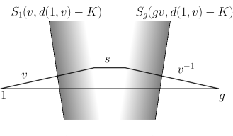
Figure 8: A quasigeodesic path

Proposition 4.3.

For any constant $T$ there is a constant $K_{9}$, which only depends on $T$, the constant of hyperbolicity $\delta$, and the relative conjugacy bounds constant, such that if $g$ is conjugate to an element $s$ of relative length at most $T$, then $g=vsv^{-1}$ for some $v$ with the following properties:

1. $d(1,v)\geqslant\tfrac{1}{2}d(1,g)-K_{9}$

2. $g\in S_{1}(v,d(1,v)-K_{9})$

3. $1\in S_{g}(gv,d(1,v)-K_{9})$

Proof.

Let $g=vsv^{-1}$, where $d(1,s)\leqslant T$ and $v$ is a conjugating element of shortest (relative) length. The first inequality follows from the triangle inequality, which implies that $d(1,v)\geqslant\tfrac{1}{2}d(1,g)-T/2$. As the path $vsv^{-1}$ is a quasigeodesic, there is a constant $L$, which only depends on $T$, the constant of hyperbolicity $\delta$, and the conjugacy bounds constant, such that the distance from $v$ to a geodesic from $1$ to $g$ is at most $L$. This implies that if $p$ is the nearest point projection of $v$ to a geodesic from $1$ to $g$, then $d(1,p)\geqslant d(1,v)-L$. As any geodesic from $v$ to $g$ is contained in a $K_{1}$-neighbourhood of the nearest point projection path, consisting of a geodesic from $v$ to $p$, and then from $p$ to $g$, where $K_{1}$ only depends on $\delta$. This implies that the distance from $1$ to any geodesic from $v$ to $g$ is at least $d(1,v)-L-K_{1}$. Finally, as the Gromov product $(v\cdot g)_{1}$ is equal to the distance from $1$ to a geodesic from $v$ to $g$, up to bounded additive error $2\delta$, this implies that $(v\cdot g)_{1}\geqslant d(1,v)-K$, where $K=L+K_{1}+2\delta$, which only depends on the constant of hyperbolicity $\delta$. This means that $g\in S_{1}(v,d(1,v)-K)$, and the same argument applied to the points $1,g$ and $vs$ implies that $1\in S_{g}(gv,d(1,v)-K)$, as $vs=gv$, for the same constant $K$. We may therefore choose $K_{9}$ to be the maximum of $K$ and $T/2$. ∎

Proposition 4.3 above shows that the probability that a random walk $w_{n}$ is conjugate to an element of relative length at most $T$, is bounded above by the probability that there is an element $v$, with $d(1,v)\geqslant\frac{1}{2}d(1,w_{n})-K_{9}$, such that $w_{n}\in S_{1}(v,d(1,v)-K_{9})$, and $w_{n}^{-1}\in S_{1}(v,d(1,v)-K_{9})$. We shall write $X_{n}$ for the measure corresponding to the distribution of pairs $(w_{n},w_{n}^{-1})$ on $\overline{G}\times\overline{G}$, i.e.

$$X_{n}(U)=\mathbb{P}((w_{n},w_{n}^{-1})\in U),$$

for any subset $U\subset\overline{G}\times\overline{G}$. As $\mathbb{P}(d(1,w_{n}))\leqslant Ln$ decays exponentially, by Theorem 1.2, this gives the following upper bound for that the probability that $w_{n}$ is conjugate to an element of length at most $T$,

$$P(\tau(w_{n})\leqslant T)\leqslant X_{n}(S_{1}(\Delta,\tfrac{1}{2}Ln-K_{9}))+O(c^{n}),$$

where $c<1$ is the constant from Theorem 1.2, and where $\Delta$ is the diagonal in $\overline{G}\times\overline{G}$.

Therefore, in order to complete the proof of Theorem 1.1, it suffices to show:

Lemma 4.4.

Let $L$ be a constant such that $\mathbb{P}(d(1,w_{n})\leqslant Ln)$ decays exponentially in $n$. Then for any $K$, there is a constant $c<1$, which depends on $K$ and $\mu$, such that

$$X_{n}(S_{1}(\Delta,\tfrac{1}{2}Ln-K))\leqslant O(c^{n}).$$

The rest of this section is devoted to the proof of Lemma 4.4. In fact, it will be convenient to obtain upper bounds for $X_{2n}$ rather than $X_{n}$. This suffices to obtain upper bounds for $X_{n}$ for all $n$, as if $D$ is the diameter of the support of $\mu$, then $X_{2n-1}(S_{1}(U,r))\leqslant X_{2n}(S_{1}(U,r-D))$, by Proposition 2.5.

We start by showing that it is very likely that a random walk $w_{2n}$ lies in the shadow $S_{1}(w_{n},\frac{1}{2}d(1,w_{n}))$.

Proposition 4.5.

The probability that $w_{2n}$ lies in $S_{1}(w_{n},\frac{1}{2}d(1,w_{n}))$ tends to one exponentially quickly as $n$ tends to infinity, i.e.

$$\mathbb{P}(w_{2n}\not\in S_{1}(w_{n},\tfrac{1}{2}d(1,w_{n})))\leqslant O(c^{n}),$$

for some $c<1$.

Proof.

We shall find an upper bound for the probability that $w_{2n}$ does not lie in the shadow $S_{1}(w_{n},\tfrac{1}{2}d(1,w_{n}))$. Conditioning on $w_{n}=g$, and using the fact that the complement of the shadow $S_{1}(w_{n},\tfrac{1}{2}d(1,w_{n}))$ is contained in $S_{w_{n}}(1,\tfrac{1}{2}d(1,w_{n})-K_{5})$, Lemma 2.8, gives

$$\mathbb{P}(w_{2n}\not\in S_{1}(w_{n},\tfrac{1}{2}d(1,w_{n})) \leqslant\sum_{g\in G}\mu_{n}(g)\mathbb{P}(gs_{n+1}\ldots s_{2n}\in S_{g}(1,\tfrac{1}{2}d(1,g)-K_{5})\mid w_{n}=g).$$

The condition $$gs_{n+1}\ldots s_{2n}\in S_{g}(1,\tfrac{1}{2}d(1,g)-K_{5}) s_{n+1}\ldots s_{2n}\in S_{1}(g^{-1},\tfrac{1}{2}d(1,g)-K_{5}) s_{n+1},\ldots,s_{2n} w_{n}$$ is the same as , and as the are independent of , this implies that

$$\mathbb{P}(w_{2n}\not\in S_{1}(w_{n},\tfrac{1}{2}d(1,w_{n})) \leqslant\sum_{g\in G}\mu_{n}(g)\mu_{n}(S_{1}(g^{-1},\tfrac{1}{2}d(1,g)-K_{5})).$$

By Theorem 1.2, the probability that $$d(1,w_{n})\leqslant Ln O(c_{1}^{n}) c_{1}<1$$ is at most , for some , which gives

$$\mathbb{P}(w_{2n}\not\in S_{1}(w_{n},\tfrac{1}{2}d(1,w_{n})) \leqslant O(c_{1}^{n})+\sum_{g\in G\setminus B(1,Ln)}\mu_{n}(g)\mu_{n}(S_{1}(g^{-1},\tfrac{1}{2}d(1,g)-K_{5})).$$

The upper bound for the measure of a shadow, Lemma 2.10, then gives the following upper bound,

$$\mathbb{P}(w_{2n}\not\in S_{1}(w_{n},\tfrac{1}{2}d(1,w_{n})) \leqslant O(c_{1}^{n})+\sum_{g\in G\setminus B(1,Ln)}\mu_{n}(g)O(c_{2}^{Ln/2-K_{5}}),$$

for some constant $$c_{2}<1$$. Therefore

$$\mathbb{P}(w_{2n}\not\in S_{1}(w_{n},\tfrac{1}{2}d(1,w_{n})) \leqslant O(c_{1}^{n})+O(c_{2}^{Ln/2}),$$

which decays exponentially in $n$, as required. ∎

Applying this result to the reflected random walk implies that the probability that $w_{2n}^{-1}$ does not lie in $S_{1}(w_{2n}^{-1}w_{n},\tfrac{1}{2}d(1,w_{2n}^{-1}w_{n}))$ also decays exponentially.

We now use this to find an upper bound for $X_{2n}$ in terms of $\mu_{n}\times\widetilde{\mu}_{n}$.

Proposition 4.6.

Let $T$ be a subset of $\overline{G}\times\overline{G}$. There are constants $L>0$ and $c<1$ such that

$$X_{2n}(S_{1}(T,r))\leqslant\mu_{n}\times\widetilde{\mu}_{n}(S_{1}(T,{\min\{r,\tfrac{1}{2}Ln\}-2\delta}))+O(c^{n}).$$

Proof.

We have shown that the probability that each of the following four events occurs tends to one exponentially quickly.

$$d(1,w_{n})\geqslant Ln$$

$$d(1,w_{2n}^{-1}w_{n})\geqslant Ln$$

$$w_{2n}\in S_{1}(w_{n},\tfrac{1}{2}d(1,w_{n}))$$

$$w_{2n}^{-1}\in S_{1}(w_{2n}^{-1}w_{n},\tfrac{1}{2}d(1,w_{2n}^{-1}w_{n}))$$

Therefore the probability that all four of them occur tends to one exponentially quickly.

If all four events occur, then $(w_{n}\cdot w_{2n})_{1}\geqslant\frac{1}{2}d(1,w_{n})\geqslant\frac{1}{2}Ln$, and similarly, $(w_{2n}^{-1}w_{n}\cdot w_{2n}^{-1})_{1}\geqslant\frac{1}{2}d(1,w_{2n}^{-1}w_{n})\geqslant\frac{1}{2}Ln$. Furthermore, if $(w_{2n},w_{2n}^{-1})$ lies in $S_{r}(T)$, then there is a point $(s,t)\in T$ such that $(w_{2n}\cdot s)_{1}\geqslant r$ and $(w_{2n}^{-1}\cdot t)_{1}\geqslant r$. This implies that $(w_{n}\cdot s)_{1}\geqslant\min\{r,\frac{1}{2}Ln\}-2\delta$, and $(w_{2n}^{-1}w_{n}\cdot t)_{1}\geqslant\min\{r,\frac{1}{2}Ln\}-2\delta$, and so $(w_{n},w_{2n}^{-1}w_{n})\in S_{1}(T,{\min\{r,\frac{1}{2}Ln\}-2\delta})$, as required. ∎

Finally, we now show that the $\mu_{n}\times\widetilde{\mu}_{n}$-measure of a shadow of the diagonal $S_{1}(\Delta,r)$ decays exponentially in $r$.

Proposition 4.7.

There are constants $c_{1}<1$ and $c_{2}<1$ such that

$$\mu_{n}\times\widetilde{\mu}_{n}(S_{1}(\Delta,r))\leqslant O(c_{1}^{r})+O(c_{2}^{n}),$$

for all $n$ and $r$.

Proof.

Let $v_{n}$ and $w_{n}$ be random walks determined by $\mu$ and $\widetilde{\mu}$ respectively. If $(v_{n},w_{n})\in S_{1}(\Delta,r)$, then there is a point $x$ such that $(v_{n}\cdot x)_{1}\geqslant r$ and $(w_{n}\cdot x)_{1}\geqslant r$. Therefore $(v_{n}\cdot w_{n})_{1}\geqslant r-2\delta$, and so $v_{n}\in S_{1}(w_{n},r-2\delta)$. By the upper bound for measures of shadows, Lemma 2.10, for any $w_{n}$ with $d(1,w_{n})\geqslant K_{6}$, the probability that $v_{n}\in S_{1}(w_{n},r-2\delta)$ is at most $K_{7}c_{1}^{r-2\delta}$, for some $c_{1}<1$. Furthermore, by Theorem 1.2, there is a $c_{2}<1$ such that the probability that $d(1,w_{n})\leqslant K_{6}$ is at most $K_{7}c_{2}^{n}$, for $n\geqslant K_{6}/L$. Therefore $\mu_{n}\times\widetilde{\mu}_{n}(S_{1}(\Delta,r))\leqslant O(c_{1}^{r})+O(c_{2}^{n})$, as required. ∎

Combining Propositions 4.6 and 4.7 establishes Lemma 4.4, and so completes the proof of Theorem 1.1.

Appendix A Chernoff-Hoeffding bounds for exponential random variables

In this section we provide the details for the following Chernoff-Hoeffding bound for exponential random variables. This proof is the solution given by Dubhashi and Panconesi to [dp]*Problem 1.10, which appeared in the initial draft version, but not in the final published version, and we reproduce it here for the sake of completeness.

Proposition A.1.

Let $Z_{i}$ be independent identically distributed exponential random variables, with expected value $Z$. Then for any $t\geqslant 0$,

$$\mathbb{P}(Z_{1}+\cdots+Z_{n}\geqslant(1+t)nZ)\leqslant\left(\frac{1+t}{e^{t}}\right)^{n}.$$

Proof.

Let $Z_{i}$ have probability density function $f(x)=\alpha e^{-\alpha x}$, so the expected value of $Z_{i}$ is $Z=1/\alpha$, and set $S_{n}=Z_{1}+\cdots+Z_{n}$. Consider the moment generating function

$$\mathbb{E}(e^{\lambda Z_{i}})=\alpha\int_{0}^{\infty}e^{\lambda x}e^{-\alpha x}dx=\frac{\alpha}{\alpha-\lambda},$$

for $0<\lambda<\alpha$. Therefore

$$\mathbb{E}(e^{\lambda S_{n}})=\left(\frac{\alpha}{\alpha-\lambda}\right)^{n}.$$

It now follows from Markov’s inequality that

$$\mathbb{P}(S_{n}\geqslant s)\leqslant\frac{\mathbb{E}(e^{\lambda S_{n}})}{e^{\lambda s}}=\frac{1}{e^{\lambda s}(1-\frac{\lambda}{\alpha})^{n}}.$$

The right hand side above is minimized by choosing $\lambda=\alpha-n/s$, which gives

$$\mathbb{P}(S_{n}\geqslant s)\leqslant\left(\frac{\alpha s}{n}\right)^{n}e^{-\alpha s+n}.$$

Setting $s=(1+t)nZ$, and using the fact that $Z=1/\alpha$, yields,

$$\mathbb{P}(S_{n}\geqslant(1+t)nZ)\leqslant\left(\frac{1+t}{e^{t}}\right)^{n},$$

as required. ∎

References

- \bibselecttransience