$\alpha$-Scale Decoupling of the Mechanical Relaxation and Diverging Shear Wave Propagation Lengthscale in Triphenylphosphite

Abstract

We have performed depolarized Impulsive Stimulated Scattering experiments to observe shear acoustic phonons in supercooled triphenylphosphite (TPP) from $\sim$10 - 500 MHz. These measurements, in tandem with previously performed longitudinal and shear measurements, permit further analyses of the relaxation dynamics of TPP within the framework of the mode coupling theory (MCT). Our results provide evidence of $\alpha$ coupling between the shear and longitudinal degrees of freedom up to a decoupling temperature $T_{c}=231~{}K$. A lower bound length scale of shear wave propagation in liquids verified the exponent predicted by theory in the vicinity of the decoupling temperature.

I Introduction

The most prominent characteristic of the frequency relaxation spectrum of glass forming liquids is the $\alpha$ peak, a broad, yet distinct feature whose origin lies in the collective degrees of freedom which undergo kinetic arrest during vitrification Binder and Kob (2005); Donth (2002); Angell et al. (2000). As the transition from liquid to glass occurs either upon cooling or the application of high pressure, the characteristic time scale of $\alpha$ relaxation varies by 16 orders of magnitude, from the $\sim$100 fs timescale associated with an attempt frequency in the liquid state Buchenau (2009) to the 100 s timescale (arbitrarily) chosen at $T_{g}$ Angell et al. (2000). One of the fundamental tasks presented to the spectroscopy of glass forming liquids is thus the complete characterization of the $\alpha$ relaxation across this span of frequencies.

To date, this challenge has best been met by dielectric spectroscopy, whose wide dynamical range remains unparalleled in the study of glass forming liquids Lunkenheimer et al. (2000); Schneider et al. (1998); Lunkenheimer et al. (2008). Nevertheless, dielectric spectroscopy of molecular liquids probes mainly orientational relaxation, while the glass transition is more naturally understood in terms of the degrees of freedom associated with flow, i.e. the density, which may be probed by longitudinal acoustic waves, and the transverse current, which couples to shear waves Balucani and Zoppi (1994); Boon and Yip (1991).

Despite the importance of both of these degrees of freedom, the bulk of the literature on structural relaxation has focussed on study of the longitudinal modulus due to the relatively limited means by which shear waves may be generated and probed. Acoustic transducer Ferry (1980); rea (1991), Impulsive Stimulated Scattering (ISS) Nelson et al. (1982); Yan and Nelson (1987); Yang and Nelson (1995) and high-frequency forced Brillouin Scattering Choi et al. (2005) techniques can continuously cover the longitudinal spectrum up to the mid-GHz regime. However, broadband shear wave generation is more accessible experimentally at lower frequencies and exhibits a gap in the range from the $\sim 10$ MHz limit of transducer methods Ferry (1980); rea (1991) to the low GHz frequencies probed by depolarized (VH) Brillouin Scattering Huang and Wang (1975); Dreyfus et al. (1999, 2003); Zhang et al. (2004); Wang et al. (1984); Tao et al. (1992). The vast majority of depolarized Brillouin Scattering studies are conducted in a single scattering geometry, permitting observation of only one acoustic wavevector. Thus, relaxation information must be extracted by complex modeling incorporating contributions from the various channels responsible for the depolarized scattering of light. Obtaining spectral information from a collection of acoustic frequencies would allow a direct determination of the shear relaxation spectrum without the need for multiparameter fitting.

Recent advancements in the generation of narrowband shear waves Torchinsky et al. (2009) using the technique of Impulsive Stimulated Brillouin Scattering (ISBS) in the depolarized geometry Nelson (1982) now permit study of the shear $\alpha$ relaxation spectrum across a broad range of frequencies. In this study, we employ ISBS to focus on tests of a first-principles theory of the glass transition, the mode coupling theory (MCT) Bengtzelius et al. (1984); Götze and Sjögren (1988); Götze (1999). While the natural variables of the theory are the density fluctuations that constitute the longitudinal modes, MCT suggests relationships among the temperature dependencies of the various relaxing variables (e.g., transverse current fluctuations, density fluctuations, orientational fluctuations, etc.) through the property of $\alpha$-scale coupling Götze (1999). This prediction states that if two variables, $A$ and $B$, couple to density fluctuations, their associated relaxation times, $\tau_{A}(T)=C_{A}\tau(T)$ and $\tau_{B}(T)=C_{B}\tau(T)$, are equivalent, up to a temperature independent factor, to a universal relaxation time $\tau(T)$ characteristic of the main $\alpha$ relaxation process. Decoupling may then occur at the MCT critical temperature $T_{c}$ when the relationship between these relaxation times can break down. Prior experimental studies that have examined $\alpha$-coupling have focused on, e.g., the coupling of dielectric to rheological variables Zorn et al. (1997), dielectric to shear mechanical relaxation Jakobsen et al. (2005), and of translational to rotational diffusion Lohfink and Sillescu (1992). However, there have been no studies that directly link elastic degrees of freedom with each other.

MCT predictions have also been formulated concerning the transverse current fluctuations in their own right, in particular the power-law divergence of an upper bound length scale for shear wave propagation derived for hard spheres in a Percus-Yevick approximation Ahluwalia and Das (1998). While such upper bound has been established in the literature Balucani and Zoppi (1994) in terms of a wavelength at which the corresponding shear acoustic frequency goes to zero, this particular scaling relationship with temperature is unique to MCT and, to our knowledge, has not undergone scrutiny in the lab.

Below, we provide a test of these assertions by building upon prior work Silence et al. (1992, 1991), and present an expanded study of the shear acoustic behavior of the fragile glass-former triphenylphosphite (TPP) ($T_{g}$ = 202 K Mizukami et al. (1999)). Taken together, these experiments fill in the gap between 10 MHz and 1 GHz in the shear relaxaiton spectrum, and thus constitute the broadest bandwidth shear acoustic measurements performed optically any glass forming system to our knowledge. Our measurement approach thus enables characterization of shear relaxation in glass-forming liquids in this frequency regime. Although supercooled liquid $\alpha$ relaxation spectra are typically broader than two decades at any temperature and, as $T$ is varied, the spectra move across many decades, the 10-1000 MHz range is sufficient to permit assessment of whether shear relaxation dynamics are consistent with relaxation dynamics determined from longitudinal wave measurements covering a comparable spectral width at common temperatures. They are also sufficient to test predictions about the low-frequency limit of shear wave propagation as a function of temperature.

We begin with a general overview of depolarized ISBS. This motivates a derivation of the signal generated in an ISBS experiment geared toward measuring shear waves from simplified versions of the hydrodynamic equations of motion. After a brief review of the experimental apparatus used, we present data collected in the temperature range from 220 K to 250 K. Our measured shear acoustic frequencies show significant acoustic dispersion, indicative of the complex relaxation dynamics characteristic of supercooled liquids thus providing a means of testing the MCT predictions described above. In particular, we see evidence of $\alpha$-decoupling, yielding an estimate of the MCT $T_{c}$ of 231 K. Using this value of the crossover temperature yields a power law for the lower limit of shear wave propagation in line with predictions derived in Ref. Ahluwalia and Das (1998). These results are discussed within the framework of the MCT.

II ISBS – General Considerations

In a typical ISS experiment, conducted in a heterodyned four-wave mixing geometry, light from a pulsed laser is incident on a diffractive optical element, typically a binary phase mask (PM) pattern, and split into two parts ($\pm 1$ diffraction orders; other orders are blocked) that are recombined at an angle $\theta$ as depicted in Fig. 1. The crossed excitation pulses generate an acoustic wave whose wavelength $\Lambda$ is given by

$$\Lambda=\frac{\lambda}{2\sin{\theta/2}}$$ (1)

where $\lambda$ is the excitation laser wavelength. Probe light (in the present case from a CW diode laser) is also incident on a phase mask pattern (the same one or another with the same spatial period) and split into two parts that are recombined at the sample to serve as probe and reference beams. The signal arises from diffraction of probe light off the acoustic wave and any other spatially periodic responses induced by the excitation pulses. The diffracted signal field is superposed with the reference field for heterodyned time-resolved detection of the signal, which typically shows damped acoustic oscillations from which the acoustic frequency and damping rate can be determined.

Figure 1: Schematic illustration of the ISS setup. Both the pump and probe beams are incident on the PM and their $\pm 1$ diffraction orders are recombined at the sample. In the case of a depolarized experiment, half-waveplates in the path of each of the four beams are used to create a polarization grating pattern in the sample plane, as shown in the figure inset.

The polarizations of the beams in the present measurements are all vertical (V) or horizontal (H) relative to the scattering plane. We denote the polarizations of the excitation fields, probe field, and reference/signal field in that order, i.e. VHVH denotes V and H excitation, V probe, and H reference and signal polarizations while VVVV denotes all V polarizations. All the measurements reported herein were conducted in the VHVH configuration.

In a depolarized (VHVH) experiment, each of the pump arms carries a different polarization and the ensuing grating is described as an alternating polarization pattern, depicted in the Fig. 1 inset. It is the regions of linear polarization that perform electrostrictive work, deforming the excited region in a fashion that generates counterpropagating shear acoustic waves with a driving force that scales with wavevector magnitude $q=2\pi/\Lambda$ Nelson (1982). The driving force also scales with a geometrical factor of $\cos{\theta/2}$ due to a diminishing of the contrast ratio of the polarization grating with increased angle. In the small $\theta$ limit, the signal from shear waves becomes markedly stronger as the wavevector is increased. In this case, the diffracted signal polarization is rotated $90^{\circ}$ from that of the incident probe light, analogous to depolarized (VH) Brillouin scattering. Finally, we note that the excitation pulses may also induce molecular orientational responses that can contribute to signal, analogous to depolarized quasielastic scattering Silence et al. (1992); Hinze et al. (2000); Pick et al. (2004); Franosch and Pick (2005); Pick et al. ; Franosch et al. (2003); Azzimani et al. (2007).

III ISBS – Theoretical Background

A full treatment of signal in an ISS experiment includes longitudinal and transverse acoustic modes, molecular orientations, and other nonoscillatory degrees of freedom Yang and Nelson (1995); Pick et al. (2004); Franosch and Pick (2005); Pick et al. ; Franosch et al. (2003); Azzimani et al. (2007); Glorieux et al. (2002). Here, we present a slightly simplified derivation that allows us to understand the presence of shear and orientational contributions to the signals.

We start with the generalized, linearized hydrodynamic equations of motion Hansen and McDonald (2006). First is the momentum density conservation law,

$$\frac{\partial}{\partial t}\rho\textbf{u}(\textbf{r},t)+\nabla\cdot\Pi(\textbf{r},t)=0$$ (2)

where $\rho$ is the density, $\textbf{u}(\textbf{r},t)$ the velocity, and $\Pi(\textbf{r},t)$ the stress tensor. The expression for the stress tensor reads

$$\Pi^{\alpha\beta}(\textbf{r},t) = \delta_{\alpha\beta}P(\textbf{r},t)-\eta\tau_{\alpha\beta}(\textbf{r},t)$$ (3)

$$+\delta_{\alpha\beta}(\frac{2}{3}\eta-\zeta)\textbf{$\nabla\cdot$ u }(\textbf{r},t)$$

$$- \mu Q_{\alpha\beta}(\textbf{r},t)+F_{\alpha\beta}(\textbf{r},t).$$

Here, $\delta_{\alpha\beta}$ is the Kronecker delta, $P(\textbf{r},t)$ is the pressure, $\eta$ is the shear viscosity, $\zeta$ is the longitudinal viscosity, $Q_{\alpha\beta}(\textbf{r},t)$ is the orientational variable, $\mu$ expresses the coupling of translational force due to rotational motion, and r is the spatial coordinate. $F_{\alpha\beta}(\textbf{r},t)$ is the external shearing stress of the laser field Ferry (1980); Wang (1980), assumed to be temporally impulsive and spatially periodic, i.e., $F_{\alpha\beta}=F_{0}^{xy}\delta(t)\cos{\textbf{q}\cdot\textbf{r}}$, and $\tau_{\alpha\beta}$ is the rate of strain, defined by

$$\tau_{\alpha\beta}=\frac{\partial u_{\alpha}(\textbf{r},t)}{\partial r_{\beta}}+\frac{\partial u_{\beta}(\textbf{r},t)}{\partial r_{\alpha}}.$$ (4)

The orientational variable obeys its own equation of motion, given by

$$\frac{\partial Q_{\alpha\beta}(\textbf{r},t)}{\partial t}=-\Gamma_{R}Q_{\alpha\beta}(\textbf{r},t)+\xi\tau_{\alpha\beta}(\textbf{r},t)+Q_{0}(\textbf{r},t)$$ (5)

where $\Gamma_{R}$ is the orientational relaxation rate, $\xi$ is the torque due to translational motion, and $Q_{0}(\textbf{r},t)$ is the torque exerted by the laser Wang (1980); Wang et al. (1984). As with the laser-induced stress, the torque will also be modeled as temporally impulsive and spatially periodic. This equation of motion assumes Debye orientational relaxation as a computational convenience.

We set the grating wavevector in the $x$ direction and the transverse direction to be $y$. Since we are interested in shear waves, we select the transverse elements of the above equations, and after a Fourier-Laplace transform defined as

$${\cal FL}\{f(\textbf{r},t)\}=\int_{0}^{\infty}dt\int_{-\infty}^{\infty}d\textbf{r}f(\textbf{r},t)e^{i\textbf{q}\cdot\textbf{r}-st},$$ (6)

we are left with

$$\rho su_{y}(\textbf{q},s) = -iq\Pi^{xy}(\textbf{q},s)$$ (7)

$$\Pi^{xy}(\textbf{q},s) = -\eta_{s}\tau^{xy}(\textbf{q},s)+F_{0}^{xy}+\mu Q_{xy}(\textbf{q},s)$$ (8)

$$sQ_{xy}(\textbf{q},s) = -\Gamma_{R}Q_{xy}(\textbf{q},s)+\xi\tau^{xy}(\textbf{q},s)+Q_{0}.$$ (9)

For simplicity, we assume that the measured signal is proportional to the molecular polarizability anisotropy Wang (1980), i.e. to $Q_{\alpha\beta}$, so we solve for the orientational variable to yield

$$Q_{xy}(\textbf{q},s)=\frac{\xi q^{2}F_{0}^{xy}+Q_{0}(s\rho+q^{2}\eta)}{(s+\Gamma_{R})(s\rho+q^{2}\eta)-\xi\mu q^{2}}.$$ (10)

In order to arrive at an analytic solution, we make the approximation that $\xi\mu q^{2}$ is a coupling of higher order that can be ignored in the solution of the equations of motion. Physically, we are making the approximation that we may ignore the recoupling of the orientational degree of freedom to itself via rotational-translational coupling. In this approximation, the expression for $Q_{xy}$ separates as

$$Q_{xy}(\textbf{q},s)=\frac{\xi q^{2}F_{0}^{xy}}{(s+\Gamma_{R})(s\rho+q^{2}\eta)}+\frac{Q_{0}}{s+\Gamma_{R}}.$$ (11)

In order to extract the effect of structural relaxation dynamics on signal, we model the $\alpha$ peak by Debye relaxation as $\frac{c_{\infty}^{2}\tau_{s}}{1+s\tau_{s}}$, where $c_{\infty}$ is the infinite frequency speed of sound and $\tau_{s}$ is the characteristic shear relaxation time. This, in effect, makes $\eta$ complex, which enables an elastic component of the shear response to emerge from the equation of motion 3 Hansen and McDonald (2006). In this model, the above equations can be solved for $Q_{xy}$ to yield

$$Q_{xy}(\textbf{q},s)=\frac{\xi q^{2}F_{0}^{xy}}{\rho}\frac{1}{(s+\Gamma_{R})(s+\frac{c_{\infty}^{2}\tau_{s}q^{2}}{1+s\tau_{s}})}+\frac{Q_{0}}{s+\Gamma_{R}}.$$ (12)

Equation (12) can be recast into the form:

$$Q_{xy}(\textbf{q},s) = \frac{\xi q^{2}F_{0}^{xy}}{\rho}\frac{2\Gamma_{s}+s}{(s+\Gamma_{R})(s+\Gamma_{s}+i\omega_{s})(s+\Gamma_{s}-i\omega_{s})}$$ (13)

$$+\frac{Q_{0}}{s+\Gamma_{R}}$$

where the shear acoustic damping rate $\Gamma_{s}$ is given by

$$\Gamma_{s}=\frac{1}{2\tau_{s}}$$ (14)

and the frequency of oscillation $\omega_{s}$ by

$$\omega_{s}=\sqrt{c_{\infty}^{2}q^{2}-\left(\frac{1}{2\tau_{s}}\right)^{2}}.$$ (15)

The acoustic damping rate $\Gamma_{s}$ thus comprises the structural relaxation dynamics. We also note that $\omega_{s}$ may go to zero for finite wavevector $q_{0}$ when

$$q_{0}=\frac{1}{2\tau_{s}c_{\infty}}.$$ (16)

Separation of equation 13 by partial fractions yields a time-domain solution

$$Q_{xy}(q,t) = \frac{\xi q^{2}F_{0}^{xy}}{\rho}[Ae^{-\Gamma_{s}t}\sin(\omega_{s}t)$$ (17)

$$+B\left(e^{-\Gamma_{R}t}-e^{-\Gamma_{s}t}\cos(\omega_{s}t)\right)]$$

$$+Q_{0}\exp(-\Gamma_{R}t)$$

where

$$A=\frac{\omega_{s}^{2}+\Gamma_{R}\Gamma_{s}-\Gamma_{s}^{2}}{\omega_{s}\left(\left(\Gamma_{s}-\Gamma_{R}\right)^{2}+\omega_{s}^{2}\right)}$$ (18)

and

$$B=\frac{(2\Gamma_{s}-\Gamma_{R})}{\left(\left(\Gamma_{s}-\Gamma_{R}\right)^{2}+\omega_{s}^{2}\right)}.$$ (19)

The solution represented by equation 17 comprises two pieces. The term proportional to $q^{2}F_{0}^{xy}$ is due to the shear acoustic response, and the other term proportional $Q_{0}$ is a decaying exponential independent of $q$. This orientational response is the optical kerr effect (OKE) signal. We also note the presence of an orientational contribution to signal in the acoustic response, due to the rotational-translational coupling.

In order to derive the relaxation spectrum from our data, we consider a frequency-dependent modulus $G^{\ast}(s)=G^{\prime}(s)+iG^{\prime\prime}(s)$ which obeys the dispersion relation Silence (1991)

$$\rho s^{2}+G(s)q^{2}=0,$$ (20)

and yields the following expressions for the real and imaginary parts of the shear modulus from the acoustic frequency and damping rate

$$G^{\prime}(\omega_{s}) = \rho\frac{\omega_{s}^{2}-\Gamma_{s}^{2}}{q^{2}}$$ (21)

$$G^{\prime\prime}(\omega_{s}) = \rho\frac{2\omega_{s}\Gamma_{s}}{q^{2}}.$$ (22)

As equation 20 has been derived considering the strain, in order to compare it with the results of the above analysis, we must solve for the strain from the original equations of motion. This gives the dispersion relation

$$\rho s^{2}+\eta sq^{2}=0.$$ (23)

Comparison between equations 20 and 23 yields the connection between the elastic modulus and the relaxation spectrum $\eta(q,\omega_{s})$

$$\frac{G^{\prime}(\omega_{s})}{\rho} = -\omega_{s}{\rm Im}[\eta(q,\omega_{s})]$$ (24)

$$\frac{G^{\prime\prime}(\omega_{s})}{\rho} = \omega_{s}{\rm Re}[\eta(q,\omega_{s})].$$ (25)

We conclude by noting that orientational responses of anisotropic molecules can be induced not only by the excitation pulses, as in the case of OKE, but also by flow that occurs due to the induced density changes Glorieux et al. (2002). Both of these sources lead to signals that can be suppressed by proper selection of probe and signal polarizations. This step was impractical when measuring shear responses, as a choice of polarization which would suppress the orientational response often reduced the already weak shear signal beyond the limit of detection. Eliminating this contribution was also deemed unnecessary, as the aim of this study was to directly probe the shear relaxation spectrum via narrowband acoustic measurements of frequencies and damping rates.

IV ISBS – Experimental Details

The pump laser system used for these studies was an Yb:KWG High-Q FemtoRegen lasing at 1035 nm and producing pulses of 500 $\mu$J at a repetition rate of 1 kHz, although 150 $\mu$J was routinely used to avoid cumulative degradation of the sample. While a 300 fs compressed pulse width FWHM was typical, we bypassed the compressor to retrieve pulses directly from the regen that were 80 ps in duration in order to avoid sample damage at high peak powers, yet remain in the impulsive limit relative to the oscillation period. The excitations beams were cylindrically focussed to a spot that was 2.5 mm in the grating wavevector dimension and 100 $\mu$m in the perpendicular dimension so that the acoustic waves would have many periods and the decay of signal would be due primarily to acoustic damping rather than propagation away from the excitation and probing region of the sample.

As a probe, we used a Sanyo DL8032-001 CW diode laser output at 830 nm with 150 mW power focused to a spot of 1 mm in the grating dimension by 50 $\mu$m in the perpendicular dimension. We also used a single phase mask optimized for diffraction into $\pm$1 order at 800 nm for both pump and probe beams, and we utilized two-lens 2:1 imaging with Thorlabs’ NIR achromats to recombine the beams at the sample. The local oscillator was attenuated by a factor of $10^{-3}$. Approximately $30\%$ of the pump power was lost into zero order with this configuration, but the pump intensity still had to be reduced significantly to avoid unwanted nonlinear effects.

In order to generate the polarization grating, we inserted $\lambda/2$ waveplates into each of the beams. These waveplates were held in precision rotation mounts to provide accurate alignment of the relative polarizations of the V and H polarized beams. This set the upper limit on the grating spacing that could be achieved in our measurements – for longer wavelengths, the beams came close enough together to be clipped by the rotation mounts. This issue was addressed by imaging with longer focal length optics. The signal was collected in a Cummings Electronics Laboratories model 3031-0003 detector and recorded by a Tektronix Model TDS-7404 oscilloscope. The shear signals were weak and required 10,000 averages, resulting in data acquisition times of a few minutes.

TPP at 97% nominal purity was purchased from Alfa Aesar and had both water and volatile impurities removed by heating under vacuum with the drying agent ${\rm MgSO_{4}}$ immersed in the liquid. The sample was then transferred to a cell with movable windows Halalay and Nelson (1990) via filtering through a millipore 0.22 $\mu$m teflon filter. After loading, the cell was placed in a Janis ST-100-H cryostat where the temperature was measured with a Lakeshore model PT-102 platinum resistor immersed directly within the liquid, and monitored and controlled with a Lakeshore 331 temperature controller.

The grating spacings examined in this study were 2.33 $\mu$m, 3.65 $\mu$m, 6.70 $\mu$m, 7.61 $\mu$m, 9.14 $\mu$m, 10.2 $\mu$m, 11.7 $\mu$m, 13.7 $\mu$m, 15.7 $\mu$m, 18.3 $\mu$m, 21.3 $\mu$m, 24.9 $\mu$m, 28.5 $\mu$m, 33.0 $\mu$m, 38.1 $\mu$m, 42.6 $\mu$m, and 50.7 $\mu$m, while data for 0.48 $\mu$m, 1.52 $\mu$m, 3.14 $\mu$m, and 4.55 $\mu$m grating spacings were taken from prior reported results Silence et al. (1992, 1991). The acoustic wavelength was calibrated through ISS measurements in ethylene glycol, for which the speed of sound is known to a high degree of accuracy Silence (1991). When the samples were cooled to the desired temperature, the cooling rate never exceeded 6 K/min, with 2 K/min being typical. Data were taken at fixed wavevector every 2 K from 220 K to 250 K upon warming as we found crystallization was less likely to occur upon warming than cooling. Only a few measurements could be taken without having to thermally cycle the liquid, as it invariably crystallized. We noticed that the tendency toward crystallization was particularly pronounced in the temperature range between 234 K and 242 K. After a few days of use, the sample was observed to develop a slightly cloudy yellowish hue, and so was replaced by a new one. The yellowish samples tended more readily toward photoinduced damage, as well as crystallization, than the original, clear samples. Comparison of the signals obtained from the degraded samples and fresh ones yielded the same frequency and damping rate values, indicating that uncertainties in either of these quantities were due mainly to noise in the data.

V Results and Discussion

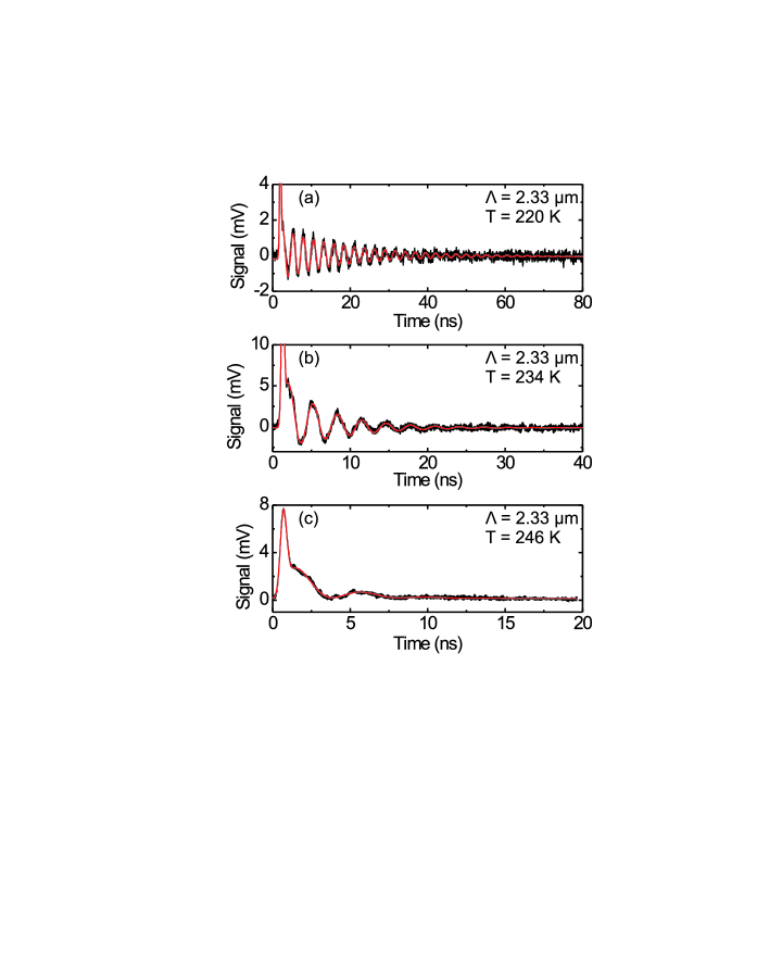
Figure 2: Shear waves in TPP with $\Lambda=2.33~{}\mu$m at (a) 220 K, (b) 234 K, and (c) 246 K. The data are in black and the fits in red. As the temperature is increased, the acoustic wave becomes more heavily damped. At higher temperatures, we also note the presence of the orientational relaxation, which appears to skew the signal such that the oscillations do not occur about the zero baseline.

The results of several VHVH experiments performed at $\Lambda$=2.33 $\mu$m grating spacing are shown in Fig. 2. There is an initial spike due to the non-resonant electronic response. Immediately following this hyperpolarizability peak are oscillations about the zero baseline from the counterpropagating shear waves. At a sample temperature of 220 K, these oscillations are seen to disappear on the scale of tens of nanoseconds due to acoustic damping. As the sample is warmed, the frequency is observed to decrease and the damping to increase dramatically. At sufficiently high temperatures, the shear wave becomes overdamped. We also note that at some temperatures, the signature of orientational relaxation is observed as a nonoscillatory decay component in the signal.

Another illustration of the influence of relaxation dynamics on the signal may be obtained by examining data from a collection of wavevectors at a common temperature, as depicted in Fig. 3 where we provide data recorded with 10.2 $\mu$m, 21.3 $\mu$m, and 44.2 $\mu$m grating spacings at 220 K. Data with a fourth wavelength, 2.33 $\mu$m, are shown in Fig. 2a. As the wavevector and the frequency are reduced, the acoustic oscillation period increases toward the characteristic relaxation timescale $\tau_{s}$ and therefore the shear wave is more heavily damped. The signals at larger grating spacings are weaker due to the linear $q$-dependence of the excitation efficiency.

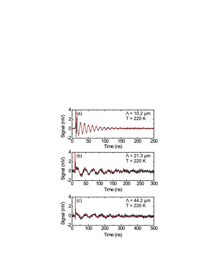
Figure 3: Shear acoustic signal in TPP at 220 K for (a) 10.2 $\mu$m, (b) 21.3 $\mu$m, and (c) 44.2 $\mu$m grating spacings. The data are in black, and the fits are in red. We note that already by 220 K at 44.2 $\mu$m, only a few acoustic cycles are observed, and that the signal intensity is reduced.

Based on the analysis of Sec. III, time-domain signals were fit to the function

$$I(t)=A^{\prime}\exp(-\Gamma_{s}t)\sin(\omega_{s}t+\phi)+B^{\prime}\exp(-\Gamma_{R}t)+C\delta(t)$$ (26)

which was convolved with the instrument response function, modelled here by a Gaussian with duration 0.262 ns. The convolution was necessary to determine the true $t=0$ for the experiment. Here, $A^{\prime}$ is the acoustic amplitude, $\Gamma_{s}$ is the shear damping rate and $\omega_{s}$ is the shear frequency. $\phi$ is a phase which accounts for the cosine term in Eq. 17, which only becomes important when the damping is strong. In the next term, $B^{\prime}$ is the optical Kerr effect signal amplitude and $\Gamma_{R}$ is the orientational relaxation rate, and in the last term $C$ is the strength of the hyperpolarizability spike. As discussed in Sec. III, it is a simplification to model the orientational behavior by a single decaying exponential Hinze et al. (2000). A more accurate description might be in terms of a Kohlrausch-Williams-Watts stretched exponential function $e^{\left(-t/tau_{s}\right)^{\beta}}$ ($0<\beta\leq 1$), as is used commonly for time-domain relaxation; however, since the orientational signal contributions are weak, we were able to obtain excellent fits with fewer parameters using a single exponential form.

The obtained values of the the shear acoustic velocity $c_{s}=\omega_{s}/q$ at a collection of wavevectors are shown in Fig. 4, while in Fig. 5 the scaled damping rates are shown. Both figures incorporate the data from Refs. Silence et al. (1992) and Silence et al. (1991). Data at other wavevectors were consistent with those shown, but are omitted from this and further plots for clarity. Two features of the data are immediately evident in these plots: first, we observe significant acoustic dispersion for the shear waves across all temperatures studied, and this dispersion increases dramatically as the temperature is raised. The second feature we note is that, as a result of the dispersion and the shear softening it represents, at each temperature above 240 K there is a wavelength above which we are unable to observe the shear wave in our measurements due to its increased damping and reduced signal strength. This wavelength is observed to decrease as temperature increases.

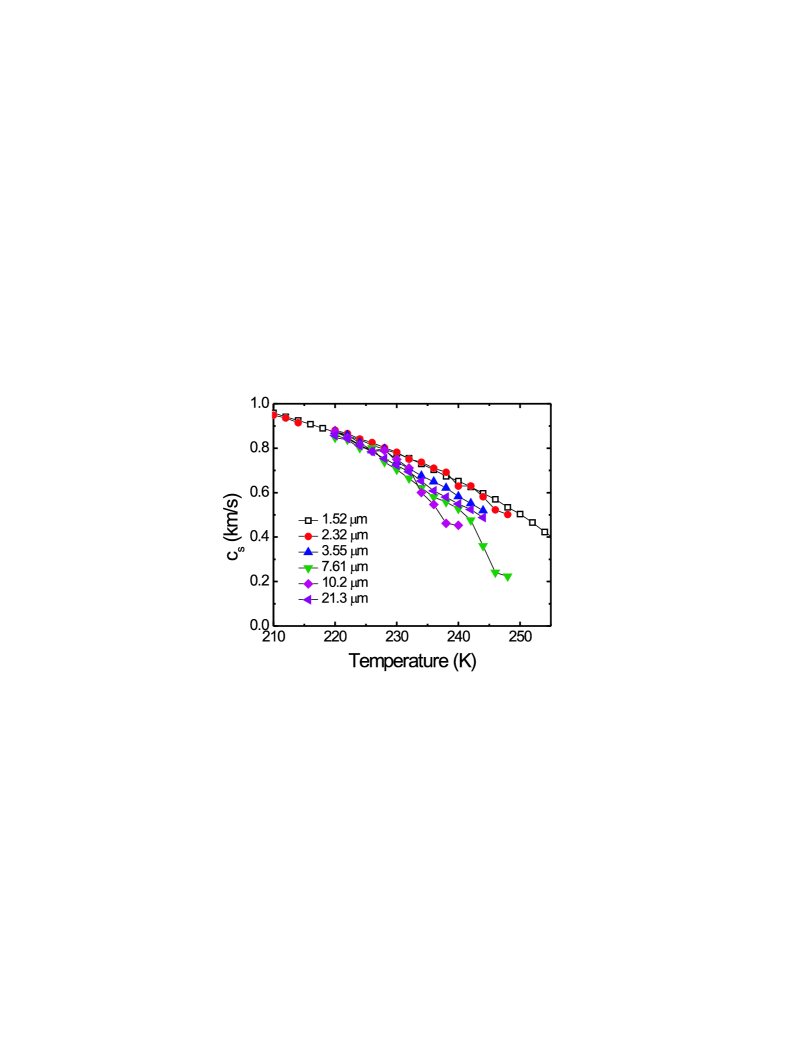
Figure 4: Shear speed of sound in TPP as a function of temperature for a variety of grating spacings. We note that the highest temperature for which we could observe shear waves increases with the decrease of grating spacing. Data at $\Lambda=~{}1.52~{}\mu$m are from Silence et al. (1992, 1991).

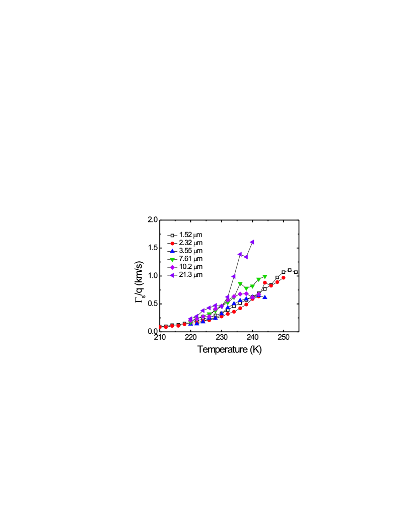
Figure 5: Scaled shear damping rate in TPP as a function of temperature for a variety of grating spacings. Longer wavelength acoustic waves have a higher scaled damping rate which increases with temperature. Data at $\Lambda=~{}1.52~{}\mu$m are from Silence et al. (1992, 1991).

From the fitted values for the shear frequency $\omega_{s}$ and the damping rate $\Gamma_{s}$, we may compute a value of the reactive and dissipative shear moduli from equations 21 and 22. The density values we obtained from data in reference Ferrer et al. (1998) were fit to a quadratic function as

$$\rho(T)=1.507~{}[{\rm g/cm^{3}}]-1.3\times 10^{-3}~{}T~{}[{\rm K}]+6.8\times 10^{-7}~{}T^{2}~{}[{\rm K^{2}}].$$ (27)

Figures 6 and 7 show plots of the real and imaginary parts of the shear modulus, respectively, as functions of temperature. These plots are for the same collection of wavevectors for which we have plotted the velocity and damping information. As in the plot of the velocity, we see the softening of the modulus at higher temperatures. The imaginary part shows generally monotonic behavior as a function of temperature as well, except for the 1.52 $\mu$m and 10.2 $\mu$m data, which show a small decrease in the imaginary part at higher temperatures, a feature which is only weakly evident in the damping rate itself represented in Fig. 5. This is likely due to the oscillation period of our shear wave exceeding the characteristic relaxation time $\tau_{s}$, permitting observation of a piece of the low-frequency side of the relaxation curve. We generally did not observe this trend at most wavevectors, as the shear wave signal became either too weak or too strongly damped to be observed.

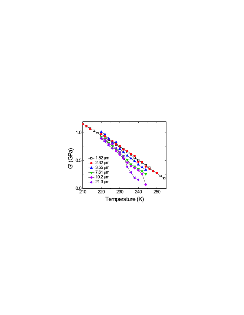
Figure 6: $G^{\prime}(T)$ at a number of grating spacings. As the temperature is increased, the shear modulus is observed to soften considerably. Again, the highest temperature for which we could observe shear waves increases with the decrease of grating spacing. Data at $\Lambda=~{}1.52~{}\mu$m are from Silence et al. (1992, 1991).

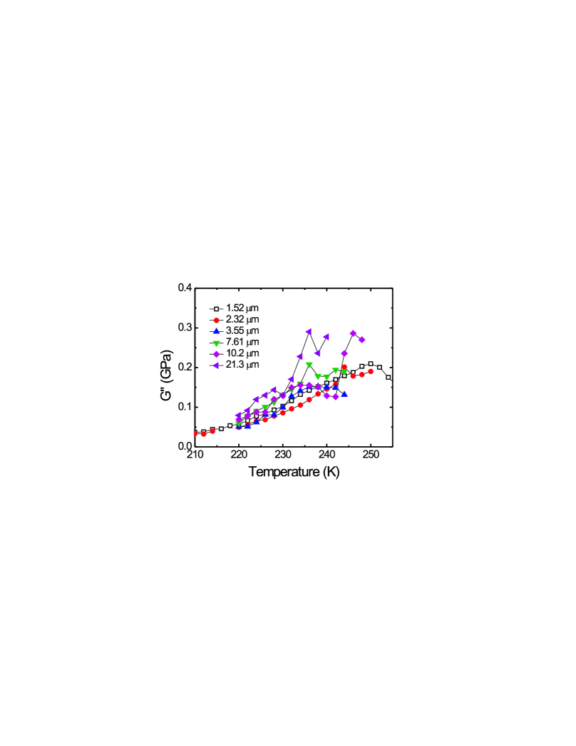
Figure 7: $G^{\prime\prime}(T)$ at a number of grating spacings. For most wavevectors examined in this study, we only observed a rise in the value of $G^{\prime\prime}(T)$ with temperature. At a handful of wavevectors, we were able to see the low-frequency side of the relaxation peak through, as is visible for $2\pi/q=1.52~{}\mu$m and $10.2~{}\mu$m. Data at $\Lambda=1.52~{}\mu$m are from Silence et al. (1992, 1991).

The moduli at each temperature were plotted as a function of frequency and then fit to the Havriliak-Negami relaxation function

$$G^{\ast}(\omega_{s})=G_{\infty}\left(1-\frac{1}{(1+(i\omega_{s}\tau_{s})^{\alpha})^{\beta}}\right)$$ (28)

in order to extract the shear relaxation spectrum ($G_{0}=0$ for all temperatures, by definition). Since time-temperature superposition has been observed to hold for $\alpha$ relaxation in many liquids and in TPP (at lower temperatures than measured here) Olsen et al. (2001), all spectra were fit simultaneously with the spectral parameters $\alpha$ and $\beta$ acting as temperature-independent global variables and $\tau_{s}$. The value for the temperature dependent infinite shear modulus $G_{\infty}=\rho c_{\infty}^{2}$ was taken from depolarized Brillouin scattering measurements performed by Chappell and Kivelson Chappell and Kivelson (1982) in a linear extrapolation to colder temperatures as

$$c_{\infty}=2620.4~{}[{\rm m/s}]-7.93T~{}[{\rm K}]$$ (29)

where the above expression has been obtained by using polarized (VV) Brillouin scattering data from longitudinal acoustic phonons to derive a temperature dependent refractive index Ferrer et al. (1998) in combination with the shear data of the reference. We note that these data fall on a common line with our lower-$T$ shear data of Fig. 6 at the highest frequencies, i.e., the shortest wavelengths ($\Lambda$ = 1.52 $\mu$m and 2.33 $\mu$m).

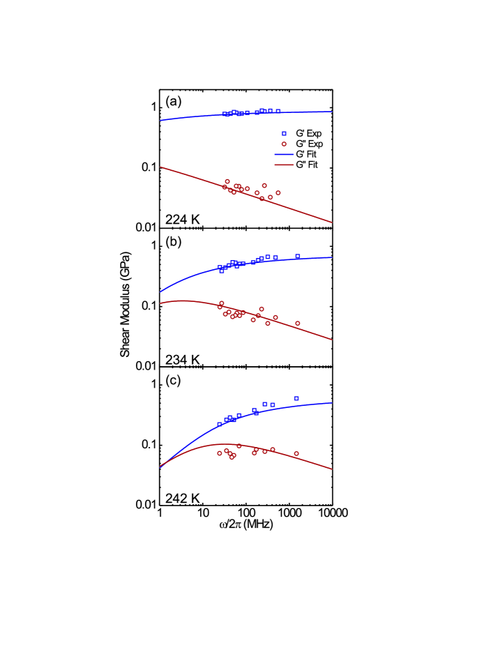
Figure 8: Plots of the real ($G^{\prime}$) and imaginary ($G^{\prime\prime}$) moduli of TPP at (a) 224 K, (b) 234 K, and (c) 242 K. At each temperature, a different segment of the shear acoustic relaxation spectrum is present within the experimental frequency window.

Three representative plots of the complex shear modulus with corresponding fits are shown in Figs. 8a - 8c. As the temperature is increased, the shear relaxation spectrum moves into the probed region. The fits produced spectral parameters $\alpha=0.61$ and $\beta=0.39$. Although not shown here, the longitudinal data from Refs. Silence et al. (1992, 1991) were refit using the same procedure for purposes of consistency and comparison, yielding spectral parameters $\alpha=0.69$ and $\beta=0.30$.

Fig. 9 presents the fitted values of $\tau_{s}$ and $\tau_{l}$ as a function of temperature along with their respective VFT fits. There is excellent agreement between the two timescales up to the temperature $T=231$ K, where the characteristic relaxation times clearly separate. When combined with the observation that the HN spectral parameters $\alpha$ and $\beta$ differ between the two degrees of freedom, we conclude that the shear acoustic wave dynamics differ significantly, at least at the lower sample temperatures measured, from those obtained from the earlier polarized ISTS data Silence et al. (1992, 1991). This conclusion, based on a larger data set taken with a broader range of acoustic wavevectors, supercedes the results of the previously published work.

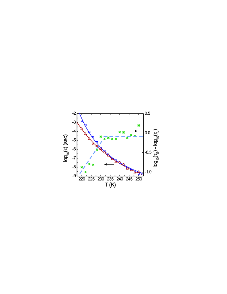
Figure 9: Characteristic relaxation time for shear ($\tau_{s}$) and longitudinal ($\tau_{l}$) degrees of freedom plotted versus temperature (left ordinate). Refitted values of the VFT parameters of the original longitudinal data are $\tau_{0}=2.5~{}\pm 1$ $\mu$s, $B=230~{}\pm 40$ K, and $T_{0}=198~{}\pm 4$ K while the shear fits produced $\tau_{0}=0.26~{}\pm 0.2$ $\mu$s, $B=450~{}\pm 240$ K, and $T_{0}=180~{}\pm 14$ K. Also shown is the decoupling parameter $\log{\tau_{s}}-\log{\tau_{l}}$ as a function of temperature (right ordinate).

We now use our data to examine the phenomenon of $\alpha$-scale coupling described briefly in the Introduction. Using the fitted values of $\tau_{s}$ and $\tau_{l}$ as a function of temperature, we define the coupling parameter as $\log{\tau_{s}}-\log{\tau_{l}}$, which is plotted alongside the relaxation time in Fig. 9. The coupling parameter is constant and essentially zero until it begins to decrease with decreasing temperature, reflecting the differing characteristic timescales of the shear and longitudinal relaxation as the former becomes slower. This provides an estimate of the MCT crossover temperature $T_{c}=231$.

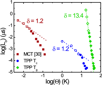
Figure 10: Computed value of length scale limit for shear wave propagation as a function of temperature $\Theta=T-T^{\prime}$ using the decoupling value for $T^{\prime}=T_{c}$ (blue circles) as the critical temperature and the glass transition temperature $T^{\prime}=T_{g}$ (green diamonds). For comparison, results from Ref. Ahluwalia and Das (1998) are also shown as a function of packing fraction $\Delta$ (red squares). The exponents are from the data plotted with empty symbols.

We may attempt to further understand our results in the mode-coupling framework of Ahluwalia and Das Ahluwalia and Das (1998). Briefly, when a calculation of a collection of hard spheres in a Percus-Yevick approximation is considered, the critical length scale $L_{0}=2\pi/q_{0}$ above which propagation of shear waves becomes overdamped obeys the power law in the vicinity of the critical control parameter

$$L_{0}=\frac{A}{(\Delta_{c}-\Delta)^{\delta}}$$ (30)

where $A=1$, $\delta=1.2$, $\Delta$ represents the packing fraction, and $\Delta_{c}$ is the MCT critical packing fraction beyond which shear wave propagation is allowed for all length scales.

Using the theoretical results of Sec. III, we may attempt to deduce a lower length scale for shear wave propagation as a function of temperature by considering at which wavevector shear wave propagation becomes overdamped. For this analysis, we chose the temperature $T$ to be the independent parameter, yielding a similar power law $L_{0}=A/(T-T^{\prime})^{\delta}$, where $T^{\prime}$ represents a critical temperature. Here we consider two significant temperatures for the liquid, i.e., the glass transition temperature $T_{g}=202$ K Mizukami et al. (1999) and the crossover temperature $T_{c}$ as determined from the MCT decoupling analysis above.

Figure 10 shows a plot of the derived upper bound, as deduced from Eq. 16 as a function of the variable $\Theta=(T-T^{\prime})$. The results of Ref. Ahluwalia and Das (1998) are also shown as a function of packing fraction $\Delta$ for comparison. A power law fit is shown to the four points in the vicinity of the relevant temperatures. Picking $T^{\prime}=T_{c}$ as the relevant temperature yields a fitted value of $\delta=1.2$, which is in excellent agreement with the theoretical result. A similar fit to the data using the literature value of $T^{\prime}=T_{g}$ produces a significantly higher value of $\delta=13.4$. We remark that the wavelength scales $L_{0}$ reached as this temperature is approached from above are several orders of magnitude larger than those corresponding to any diverging structural correlation length scale.

VI Conclusions

We have used depolarized impulsive stimulated Brillouin scattering to measure shear acoustic waves in supercooled triphenyl phosphite from 220 K to 250 K combined with previously obtained results, we are able to examine a frequency regime from $\sim 10$ MHz to almost $1$ GHz. Our results indicate that the shear and longitudinal spectra do not share the same spectral parameters $\alpha$ and $\beta$.

We also observed $\alpha$-decoupling of the longitudinal and shear degrees of freedom, yielding an estimate of the mode-coupling $T_{c}=231$ K. Using the decoupling result, we verified a power law for the diverging lengthscale of shear wave propagation as $\delta=1.24$. A similar test using the literature value of $T_{g}$ was not in agreement with the theoretical model, as should be expected since $T_{g}$ is not a mode-coupling theory parameter.

Further work in the study of shear relaxation in triphenyl phosphite and other liquids will center on expanding the dynamic range of the measurements. We also note that a comparison with dielectric data via the model of DiMarzio and Bishop Dimarzio and Bishop (1974) could also be performed if dielectric relaxation measurements at a similar combination of temperatures and frequencies were carried out.

VII Acknowledgments

We gratefully acknowledge Professor Shankar P. Das for useful discussions. This work was supported in part by National Science Foundation Grants No. CHE-0616939 and IMR-0414895.

References

- Binder and Kob (2005) K. Binder and W. Kob, Glassy Materials and Disordered Solids – An Introduction to Theiry Statistical Mechanics (World Scientific Publishing Co. Pte. Ltd., 2005).
- Donth (2002) E. Donth, The Glass Transition (Springer,Berlin, 2002).
- Angell et al. (2000) C. A. Angell, K. L. Ngai, G. B. McKenna, P. F. McMillan, and S. W. Martin, J. Appl. Phys., 88, 3113 (2000).
- Buchenau (2009) U. Buchenau, Private Communication (2009).
- Lunkenheimer et al. (2000) P. Lunkenheimer, U. Schneider, R. Brand, and A. Loidl, Contemp. Phys., 41, 15 (2000).
- Schneider et al. (1998) U. Schneider, P. Lunkenheimer, R. Brand, and A. Loidl, J. Non-Cryst. Solids, 235-237, 173 (1998).
- Lunkenheimer et al. (2008) P. Lunkenheimer, L. C. Pardo, M. Koehler, and A. Loidl, Phys. Rev. E, 77, 031506 (2008).
- Balucani and Zoppi (1994) U. Balucani and M. Zoppi, Dynamics of the Liquid State (Oxford University Press, 1994).
- Boon and Yip (1991) J. P. Boon and S. Yip, Molecular Hydrodynamics (Dover Publications, Inc., 1991).
- Ferry (1980) J. D. Ferry, Viscoelastic Properties of Polymers, 3rd ed. (Wiley, 1980).
- rea (1991) “Physical methods of chemistry,” (Wiley, 1991) p. 1, 2nd ed.
- Nelson et al. (1982) K. A. Nelson, R. J. D. Miller, D. R. Lutz, and M. D. Fayer, J. Appl. Phys., 53, 1144 (1982).
- Yan and Nelson (1987) Y.-X. Yan and K. A. Nelson, J. Chem. Phys., 87, 6240 (1987).
- Yang and Nelson (1995) Y. W. Yang and K. A. Nelson, J. Chem. Phys., 103, 7722 (1995).
- Choi et al. (2005) J. D. Choi, T. Feurer, M. Yamaguchi, B. Paxton, and K. A. Nelson, Appl. Phys. Lett., 87, 081907 (2005).
- Huang and Wang (1975) Y. Y. Huang and C. H. Wang, J. Chem. Phys., 62, 120 (1975).
- Dreyfus et al. (1999) C. Dreyfus, A. Aouadi, R. M. Pick, T. Berger, A. Patkowski, and W. Steffen, Eur. Phys. J. B, 9, 401 (1999).
- Dreyfus et al. (2003) C. Dreyfus, A. Aouadi, J. Gapinski, M. Matos-Lopes, W. Steffen, A. Patkowski, and R. M. Pick, Phys. Rev. E, 68, 011204 (2003).
- Zhang et al. (2004) H. P. Zhang, A. Brodin, H. C. Barshilia, G. Q. Shen, H. Z. Cummins, and R. M. Pick, Phys. Rev. E, 70, 011502 (2004).
- Wang et al. (1984) C. H. Wang, R.-J. Ma, and Q.-L. Liu, J. Chem. Phys., 80, 617 (1984).
- Tao et al. (1992) N. J. Tao, G. Li, and H. Z. Cummins, Phys. Rev. B, 45, 686 (1992).
- Torchinsky et al. (2009) D. H. Torchinsky, J. A. Johnson, and K. A. Nelson, J. Chem. Phys., 130, 064502 (2009).
- Nelson (1982) K. A. Nelson, J. Appl. Phys., 53, 6060 (1982).
- Bengtzelius et al. (1984) U. Bengtzelius, W. Goetze, and A. Sjolander, J. Phys., C17, 5915 (1984).
- Götze and Sjögren (1988) W. Götze and L. Sjögren, J. Phys. C: Solid State Phys., 21, 3407 (1988).
- Götze (1999) W. Götze, J. Phys.: Condens. Matter, 11, A1 (1999).
- Zorn et al. (1997) R. Zorn, F. I. Mopsik, G. B. McKenna, L. Willner, and D. Richter, J. Chem. Phys., 107, 3645 (1997).
- Jakobsen et al. (2005) B. Jakobsen, K. Niss, and N. B. Olsen, J. Chem. Phys., 123, 234511 (2005).
- Lohfink and Sillescu (1992) M. Lohfink and H. Sillescu, in AIP Conf. Proc. No. 256, American Institute of Physics (American Institute of Physics, New York, 1992).
- Ahluwalia and Das (1998) R. Ahluwalia and S. P. Das, Phys. Rev. E, 57, 5771 (1998).
- Silence et al. (1992) S. M. Silence, A. R. Duggal, L. Dhar, and K. A. Nelson, J. Chem. Phys., 96, 5448 (1992).
- Silence et al. (1991) S. M. Silence, S. R. Goates, and K. A. Nelson, J. Non-Cryst. Solids, 131, 37 (1991).
- Mizukami et al. (1999) M. Mizukami, K. Kobashi, M. Hanaya, and M. Oguni, J. Phys. Chem. B, 103, 4078 (1999).
- Hinze et al. (2000) G. Hinze, D. D. Brace, S. D. Gottke, and M. D. Fayer, J. Chem. Phys., 113, 3723 (2000).
- Pick et al. (2004) R. M. Pick, C. Dreyfus, A. Azzimani, R. Gupta, R. Torre, A. Taschin, and T. Franosch, Eur. Phys. J. B, 39, 169 (2004).
- Franosch and Pick (2005) T. Franosch and R. M. Pick, Eur. Phys. J. B, 47, 341 (2005).
- (37) R. M. Pick, T. Franosch, A. Latz, and C. Dreyfus, Eur. Phys. J. B, 31, 217.
- Franosch et al. (2003) T. Franosch, A. Latz, and R. M. Pick, Eur. Phys. J. B, 31, 229 (2003).
- Azzimani et al. (2007) A. Azzimani, C. Dreyfus, R. M. Pick, P. Bartolini, A. Taschin, and R. Torre, Phys. Rev. E, 76, 011509 (2007).
- Glorieux et al. (2002) C. Glorieux, K. A. Nelson, G. Hinze, and M. D. Fayer, J. Chem. Phys., 116, 3384 (2002).
- Hansen and McDonald (2006) J.-P. Hansen and I. R. McDonald, Theory of Simple Liquids, 3rd ed. (Elsevier, 2006).
- Wang (1980) C. H. Wang, Mol. Phys., 41, 541 (1980).
- Silence (1991) S. Silence, Ph.D. thesis, Massachusetts Institute of Technology (1991).
- Halalay and Nelson (1990) I. C. Halalay and K. A. Nelson, Rev. Sci. Instrum., 61, 3623 (1990).
- Ferrer et al. (1998) M. L. Ferrer, C. Lawrence, B. G. Demirjian, D. Kivelson, C. Alba-Simionesco, and G. Tarjus, J. Chem. Phys., 109, 8010 (1998).
- Olsen et al. (2001) N. B. Olsen, T. Christensen, and J. C. Dyre, Phys. Rev. Lett., 86, 1271 (2001).
- Chappell and Kivelson (1982) P. J. Chappell and D. Kivelson, J. Chem. Phys., 76, 1742 (1982).
- Dimarzio and Bishop (1974) E. A. Dimarzio and M. Bishop, J. Chem. Phys., 60, 3802 (1974).