Distributed Stochastic Optimization with Centralized Control
Abstract
We analyze the convergence of gradient-based optimization algorithms that base their updates on delayed stochastic gradient information. The main application of our results is to the development of gradient-based distributed optimization algorithms where a master node performs parameter updates while worker nodes compute stochastic gradients based on local information in parallel, which may give rise to delays due to asynchrony. We take motivation from statistical problems where the size of the data is so large that it cannot fit on one computer; with the advent of huge datasets in biology, astronomy, and the internet, such problems are now common. Our main contribution is to show that for smooth stochastic problems, the delays are asymptotically negligible and we can achieve order-optimal convergence results. In application to distributed optimization, we develop procedures that overcome communication bottlenecks and synchronization requirements. We show -node architectures whose optimization error in stochastic problems—in spite of asynchronous delays—scales asymptotically as after iterations. This rate is known to be optimal for a distributed system with nodes even in the absence of delays. We additionally complement our theoretical results with numerical experiments on a statistical machine learning task.
Distributed Delayed Stochastic Optimization
Alekh Agarwal John C. Duchi
{alekh,jduchi}@eecs.berkeley.edu
Department of Electrical Engineering and Computer Sciences
University of California, Berkeley
1 Introduction
We focus on stochastic convex optimization problems of the form
| (1) |
where is a closed convex set, is a probability distribution over , and is convex for all , so that is convex. The goal is to find a parameter that approximately minimizes over . Classical stochastic gradient algorithms [RM51, Pol87] iteratively update a parameter by sampling , computing , and performing the update , where denotes projection onto the set . In this paper, we analyze asynchronous gradient methods, where instead of receiving current information , the procedure receives out of date gradients , where is the (potentially random) delay at time . The central contribution of this paper is to develop algorithms that—under natural assumptions about the functions in the objective (1)—achieve asymptotically optimal rates for stochastic convex optimization in spite of delays.
Our model of delayed gradient information is particularly relevant in distributed optimization scenarios, where a master maintains the parameters while workers compute stochastic gradients of the objective (1). The architectural assumption of a master with several worker nodes is natural for distributed computation, and other researchers have considered models similar to those in this paper [NBB01, LSZ09]. By allowing delayed and asynchronous updates, we can avoid synchronization issues that commonly handicap distributed systems.
Certainly distributed optimization has been studied for several decades, tracing back at least to seminal work of Tsitsiklis and colleagues ([Tsi84, BT89]) on minimization of smooth functions where the parameter vector is distributed. More recent work has studied problems in which each processor or node in a network has a local function , and the goal is to minimize the sum [NO09, RNV10, JRJ09, DAW10]. Most prior work assumes as a constraint that data lies on several different nodes throughout a network. However, as Dekel et al. [DGBSX10a] first noted, in distributed stochastic settings independent realizations of a stochastic gradient can be computed concurrently, and it is thus possible to obtain an aggregated gradient estimate with lower variance. Using modern stochastic optimization algorithms (e.g. [JNT08, Lan10]), Dekel et al. give a series of reductions to show that in an -node network it is possible to achieve a speedup of over a single-processor so long as the objective is smooth.
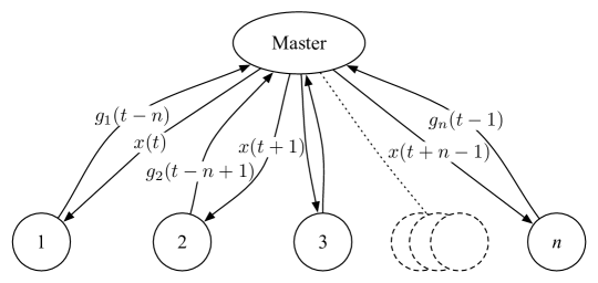
Our work is closest to Nedić et al.’s asynchronous subgradient method [NBB01], which is an incremental gradient procedure in which gradient projection steps are taken using out-of-date gradients. See Figure 1 for an illustration. The asynchronous subgradient method performs non-smooth minimization and suffers an asymptotic penalty in convergence rate due to the delays: if the gradients are computed with a delay of , then the convergence rate of the procedure is . The setting of distributed optimization provides an elegant illustration of the role played by the delay in convergence rates. As in Fig. 1, the delay can essentially be of order in Nedić et al.’s setting, which gives a convergence rate of . A simple centralized stochastic gradient algorithm attains a rate of , which suggests something is amiss in the distributed algorithm. Langford et al. [LSZ09] rediscovered Nedić et al.’s results and attempted to remove the asymptotic penalty by considering smooth objective functions, though their approach has a technical error (see Appendix C), and even so they do not demonstrate any provable benefits of distributed computation. We analyze similar asynchronous algorithms, but we show that for smooth stochastic problems the delay is asymptotically negligible—the time does not matter—and in fact, with parallelization, delayed updates can give provable performance benefits.
We build on results of Dekel et al. [DGBSX10a], who show that when the objective has Lipschitz-continuous gradients, then when processors compute stochastic gradients in parallel using a common parameter it is possible to achieve convergence rate so long as the processors are synchronized (under appropriate synchrony conditions, this holds nearly independently of network topology). A variant of their approach is asymptotically robust to asynchrony so long as most processors remain synchronized for most of the time [DGBSX10b]. We show results similar to their initial discovery, but we analyze the effects of asynchronous gradient updates where all the nodes in the network can suffer delays. Application of our main results to the distributed setting provides convergence rates in terms of the number of nodes in the network and the stochastic process governing the delays. Concretely, we show that under different assumptions on the network and delay process, we achieve convergence rates ranging from to , which is asymptotically in . For problems with large , we demonstrate faster rates ranging from to . In either case, the time necessary to achieve -optimal solution to the problem (1) is asymptotically , a factor of —the size of the network—better than a centralized procedure in spite of delay.
The remainder of the paper is organized as follows. We begin by reviewing known algorithms for solving the stochastic optimization problem (1) and stating our main assumptions. Then in Section 3 we give abstract descriptions of our algorithms and state our main theoretical results, which we make concrete in Section 4 by formally placing the analysis in the setting of distributed stochastic optimization. We complement the theory in Section 5 with experiments on a real-world dataset, and proofs follow in the remaining sections.
Notation
For the reader’s convenience, we collect our (mostly standard) notation here. We denote general norms by , and the dual norm to the norm is defined as . The subdifferential set of a function is
We use the shorthand . A function is -Lipschitz with respect to the norm on if for all , . For convex , this is equivalent to for all (e.g. [HUL96a]). A function is -smooth on if is Lipschitz continuous with respect to the norm , defined as
For convex differentiable , the Bregman divergence [Bre67] between and is defined as
| (2) |
A convex function is -strongly convex with respect to a norm over if
| (3) |
We use to denote the set of integers .
2 Setup and Algorithms
In this section we set up and recall the delay-free algorithms underlying our approach. We then give the appropriate delayed versions of these algorithms, which we analyze in the sequel.
2.1 Setup and Delay-free Algorithms
To build intuition for the algorithms we analyze, we first describe two closely related first-order algorithms: the dual averaging algorithm of Nesterov [Nes09] and the mirror descent algorithm of Nemirovski and Yudin [NY83], which is analyzed further by Beck and Teboulle [BT03]. We begin by collecting notation and giving useful definitions. Both algorithms are based on a proximal function , where it is no loss of generality to assume that for all . We assume is -strongly convex (by scaling, this is no loss of generality). By definitions (2) and (3), the divergence satisfies .
In the oracle model of stochastic optimization that we assume, at time both algorithms query an oracle at the point , and the oracle then samples i.i.d. from the distribution and returns . The dual averaging algorithm [Nes09] updates a dual vector and primal vector via
| (4) |
while mirror descent [NY83, BT03] performs the update
| (5) |
Both make a linear approximation to the function being minimized—a global approximation in the case of the dual averaging update (4) and a more local approximation for mirror descent (5)—while using the proximal function to regularize the points .
We now state the two essentially standard assumptions [JNT08, Lan10, Xia10] we most often make about the stochastic optimization problem (1), after which we recall the convergence rates of the algorithms (4) and (5).
Assumption A (Lipschitz Functions).
For -a.e. , the function is convex. Moreover, for any , .
In particular, Assumption A implies that is -Lipschitz continuous with respect to the norm and that is convex. Our second assumption has been used to show rates of convergence based on the variance of a gradient estimator for stochastic optimization problems (e.g. [JNT08, Lan10]).
Assumption B (Smooth Functions).
Several commonly used functions satisfy the above assumptions, for example:
- (i)
- (ii)
We also make a standard compactness assumption on the optimization set .
Assumption C (Compactness).
For and , the bounds and both hold.
Under Assumptions A or B in addition to Assumption C, the updates (4) and (5) have known convergence rates. Define the time averaged vector as
| (6) |
Then under Assumption A, both algorithms satisfy
| (7) |
for the stepsize choice (e.g. [Nes09, Xia10, NJLS09]). The result (7) is sharp to constant factors in general [NY83, ABRW10], but can be further improved under Assumption B. Building on work of Juditsky et al. [JNT08] and Lan [Lan10], Dekel et al. [DGBSX10a, Appendix A] show that under Assumptions B and C the stepsize choice , where is a damping factor set to , yields for either of the updates (4) or (5) the convergence rate
| (8) |
2.2 Delayed Optimization Algorithms
We now turn to extending the dual averaging (4) and mirror descent (5) updates to the setting in which instead descent (5) updates to the setting in which instead of receiving a current gradient at time , the procedure receives a gradient , that is, a stochastic gradient of the objective (1) computed at the point . In the simplest case, the delays are uniform and for all , but in general the delays may be a non-i.i.d. stochastic process. Our analysis admits any sequence of delays as long as the mapping satisfies . We also require that each update happens once, i.e., is one-to-one, though this second assumption is easily satisfied.
Recall that the problems we consider are stochastic optimization problems of the form (1). Under the assumptions above, we extend the mirror descent and dual averaging algorithms in the simplest way: we replace with . For dual averaging (c.f. the update (4)) this yields
| (9) |
while for mirror descent (c.f. the update (5)) we have
| (10) |
A generalization of Nedić et al.’s results [NBB01] by combining their techniques with the convergence proofs of dual averaging [Nes09] and mirror descent [BT03] is as follows. Under Assumptions A and C, so long as for all , choosing gives rate
| (11) |
3 Convergence rates for delayed optimization of smooth functions
In this section, we state and discuss several results for asynchronous stochastic gradient methods. We give two sets of theorems. The first are for the asynchronous method when we make updates to the parameter vector using one stochastic subgradient, according to the update rules (9) or (10). The second method involves using several stochastic subgradients for every update, each with a potentially different delay, which gives sharper results that we present in Section 3.2.
3.1 Simple delayed optimization
Intuitively, the -penalty due to delays for non-smooth optimization arises from the fact that subgradients can change drastically when measured at slightly different locations, so a small delay can introduce significant inaccuracy. To overcome the delay penalty, we now turn to the smoothness assumption B as well as the Lipschitz condition A (we assume both of these conditions along with Assumption C hold for all the theorems). In the smooth case, delays mean that stale gradients are only slightly perturbed, since our stochastic algorithms constrain the variability of the points . As we show in the proofs of the remaining results, the error from delay essentially becomes a second order term: the penalty is asymptotically negligible. We study both update rules (9) and (10), and we set . Here will be chosen to both control the effects of delays and for errors from stochastic gradient information. We prove the following theorem in Sec. 6.1.
Theorem 1.
Let the sequence be defined by the update (9). Define the stepsize or let for all . Then
The mirror descent update (10) exhibits similar convergence properties, and we prove the next theorem in Sec. 6.2.
In each of the above theorems, we can set . As immediate corollaries, we recall the definition (6) of the averaged sequence of and use convexity to see that
for either update rule. In addition, we can allow the delay to be random:
Corollary 1.
We provide the proof of the corollary in Sec. 6.3. The take-home message from the above corollaries, as well as Theorems 1 and 2, is that the penalty in convergence rate due to the delay is asymptotically negligible. As we discuss in greater depth in the next section, this has favorable implications for robust distributed stochastic optimization algorithms.
3.2 Combinations of delays
In some scenarios—including distributed settings similar to those we discuss in the next section—the procedure has access not to only a single delayed gradient but to several with different delays. To abstract away the essential parts of this situation, we assume that the procedure receives gradients , where each has a potentially different delay . Now let belong to the probability simplex, though we leave ’s values unspecified for now. Then the procedure performs the following updates at time : for dual averaging,
| (12) |
while for mirror descent, the update is
| (13) |
The next two theorems build on the proofs of Theorems 1 and 2, combining several techniques. We provide the proof of Theorem 3 in Sec. 7, omitting the proof of Theorem 4 as it follows in a similar way from Theorem 2.
Theorem 3.
Theorem 4.
4 Distributed Optimization
We now turn to what we see as the main purpose and application of the above results: developing robust and efficient algorithms for distributed stochastic optimization. Our main motivations here are machine learning and statistical applications where the data is so large that it cannot fit on a single computer. Examples of the form (1) include logistic regression (for background, see [HTF01]), where the task is to learn a linear classifier that assigns labels in to a series of examples, in which case we have the objective as described in Sec. 2.1(i); or linear regression, where and as described in Sec. 2.1(ii). Both objectives satisfy assumptions A and B as discussed earlier. We consider both stochastic and online/streaming scenarios for such problems. In the simplest setting, the distribution in the objective (1) is the empirical distribution over an observed dataset, that is,
We divide the samples among workers so that each worker has an -sized subset of data. In streaming applications, the distribution is the unknown distribution generating the data, and each worker receives a stream of independent data points . Worker uses its subset of the data, or its stream, to compute , an estimate of the gradient of the global . We make the simplifying assumption that is an unbiased estimate of , which is satisfied, for example, when each worker receives an independent stream of samples or computes the gradient based on samples picked at random without replacement from its subset of the data.
The architectural assumptions we make are natural and based off of master/worker topologies, but the convergence results in Section 3 allow us to give procedures robust to delay and asynchrony. We consider two protocols: in the first, workers compute and communicate asynchronously and independently with the master, and in the second, workers are at different distances from the master and communicate with time lags proportional to their distances. We show in the latter part of this section that the convergence rates of each protocol, when applied in an -node network, are for -node networks (though lower order terms are different for each).
Before describing our architectures, we note that perhaps the simplest master-worker scheme is to have each worker simultaneously compute a stochastic gradient and send it to the master, which takes a gradient step on the averaged gradient. While the gradients are computed in parallel, accumulating and averaging gradients at the master takes time, offsetting the gains of parallelization. Thus we consider alternate architectures that are robust to delay.
Cyclic Delayed Architecture
This protocol is the delayed update algorithm mentioned in the introduction, and it parallelizes computation of (estimates of) the gradient . Formally, worker has parameter and computes , where is a random variable sampled at worker from the distribution . The master maintains a parameter vector . The algorithm proceeds in rounds, cyclically pipelining updates. The algorithm begins by initiating gradient computations at different workers at slightly offset times. At time , the master receives gradient information at a -step delay from some worker, performs a parameter update, and passes the updated central parameter back to the worker. Other workers do not see this update and continue their gradient computations on stale parameter vectors. In the simplest case, each node suffers a delay of , though our earlier analysis applies to random delays throughout the network as well. Recall Fig. 1 for a graphic description of the process.
 |
 |
| (a) | (b) |
Locally Averaged Delayed Architecture
At a high level, the protocol we now describe combines the delayed updates of the cyclic delayed architecture with averaging techniques of previous work [NO09, DAW10]. We assume a network , where is a set of nodes (workers) and are the edges between the nodes. We select one of the nodes as the master, which maintains the parameter vector over time.
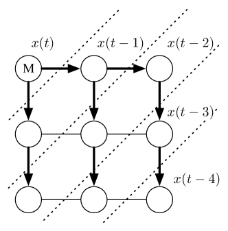
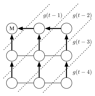
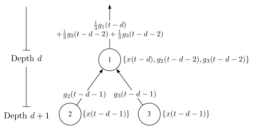
The algorithm works via a series of multicasting and aggregation steps on a spanning tree rooted at the master node. In the first phase, the algorithm broadcasts from the root towards the leaves. At step the master sends its current parameter vector to its immediate neighbors. Simultaneously, every other node broadcasts its current parameter vector (which, for a depth node, is ) to its children in the spanning tree. See Fig. 2(a). Every worker receives its new parameter and computes its local gradient at this parameter. The second part of the communication in a given iteration proceeds from leaves toward the root. The leaf nodes communicate their gradients to their parents. The parent takes the gradients of the leaf nodes from the previous round (received at iteration ) and averages them with its own gradient, passing this averaged gradient back up the tree. Again simultaneously, each node takes the averaged gradient vectors of its children from the previous rounds, averages them with its current gradient vector, and passes the result up the spanning tree. See Fig. 2(b) and Fig. 3 for a visual description.
Slightly more formally, associated with each node is a delay , which is (generally) twice its distance from the master. Fix an iteration . Each node has an out of date parameter vector , which it sends further down the tree to its children. So, for example, the master node sends the vector to its children, which send the parameter vector to their children, which in turn send to their children, and so on. Each node computes
where is a random variable sampled at node from the distribution . The communication back up the hierarchy proceeds as follows: the leaf nodes in the tree (say at depth ) send the gradient vectors to their immediate parents in the tree. At the previous iteration , the parent nodes received from their children, which they average with their own gradients and pass to their parents, and so on. The master node at the root of the tree receives an average of delayed gradients from the entire tree, with each gradient having a potentially different delay, giving rise to updates of the form (12) or (13).
4.1 Convergence rates for delayed distributed minimization
Having described our architectures, we can now give corollaries to the theoretical results from the previous sections that show it is possible to achieve asymptotically faster rates (over centralized procedures) using distributed algorithms even without imposing synchronization requirements. We allow workers to pipeline updates by computing asynchronously and in parallel, so each worker can compute low variance estimate of the gradient .
We begin with a simple corollary to the results in Sec. 3.1. We ignore the constants , , , and , which are not dependent on the characteristics of the network. We also assume that each worker uses independent samples of to compute the stochastic gradient as
Using the cyclic protocol as in Fig. 1, Theorems 1 and 2 give the following result.
Corollary 2.
Proof The corollary follows straightforwardly from the realization that the variance when workers use independent stochastic gradient samples. ∎
In the above corollary, so long as the bound on the delay satisfies, say, , then the last term in the bound is asymptotically negligible, and we achieve a convergence rate of .
The cyclic delayed architecture has the drawback that information from a worker can take time to reach the master. While the algorithm is robust to delay and does not need lock-step coordination of workers, the downside of the architecture is that the essentially term in the bounds above can be quite large. Indeed, if each worker computes its gradient over samples with —say to avoid idling of workers—then the cyclic architecture has convergence rate . For moderate or large , the delay penalty may dominate , offsetting the gains of parallelization.
To address the large drawback, we turn our attention to the locally averaged architecture described by Figs. 2 and 3, where delays can be smaller since they depend only on the height of a spanning tree in the network. The algorithm requires more synchronization than the cyclic architecture but still performs limited local communication. Each worker computes where is the delay of worker from the master and . As a result of the communication procedure, the master receives a convex combination of the stochastic gradients evaluated at each worker , for which we gave results in Section 3.2.
In this architecture, the master receives gradients of the form for some in the simplex, which puts us in the setting of Theorems 3 and 4. We now make the reasonable assumption that the gradient errors are uncorrelated across the nodes in the network.222Similar results continue to hold under weak correlation. In statistical applications, for example, each worker may own independent data or receive streaming data from independent sources; more generally, each worker can simply receive independent samples . We also set , and observe
Corollary 3.
The multiplier can be reduced to a constant if we set . By using the averaged sequence (6), Jensen’s inequality gives that asymptotically , which is an optimal dependence on the number of samples calculated by the method. We also observe in this architecture, the delay is bounded by the graph diameter , giving us the bound:
| (14) |
The above corollaries are general and hold irrespective of the relative costs of communication and computation. However, with knowledge of the costs, we can adapt the stepsizes slightly to give better rates of convergence when is large or communication to the master node is expensive. For now, we focus on the cyclic architecture (the setting of Corollary 2), though the same principles apply to the local averaging scheme. Let denote the cost of communicating between the master and workers in terms of the time to compute a single gradient sample, and assume that we set , so that no worker node has idle time. For simplicity, we let the delay be non-random, so . Consider the choice for the damping stepsizes, where . This setting in Theorem 1 gives
where the last equality follows since . Optimizing for on the right yields
| (15) |
The convergence rates thus follow two regimes. When , we have convergence rate , while once , we attain convergence. Roughly, in time proportional to , we achieve optimization error , which is order-optimal given that we can compute a total of stochastic gradients [ABRW10]. The scaling of this bound is nicer than that previously: the dependence on network size is at worst , which we obtain by increasing the damping factor —and hence decreasing the stepsize —relative to the setting of Corollary 2. We remark that applying the same technique to Corollary 3 gives convergence rate scaling as the smaller of and . Since the diameter , this is faster than the cyclic architecture’s bound (15).
4.2 Running-time comparisons
Having derived the rates of convergence of the different distributed procedures above, we now explicitly study the running times of the centralized stochastic gradient algorithms (4) and (5), the cyclic delayed protocol with the updates (9) and (10), and the locally averaged architecture with the updates (12) and (13). To make comparisons more cleanly, we avoid constants, assuming without loss that the variance bound on is , and that sampling and evaluating requires one unit of time. Noting that , it is clear that if we receive uncorrelated samples of , the variance .
Now we state our assumptions on the relative times used by each algorithm. Let be the number of units of time allocated to each algorithm, and let the centralized, cyclic delayed and locally averaged delayed algorithms complete , and iterations, respectively, in time . It is clear that . We assume that the distributed methods use and samples of to compute stochastic gradients and that the delay of the cyclic algorithm is . For concreteness, we assume that communication is of the same order as computing the gradient of one sample so that . In the cyclic setup of Sec. 3.1, it is reasonable to assume that to avoid idling of workers (Theorems 1 and 2, as well as the bound (15), show it is asymptotically beneficial to have larger, since ). For , the master requires units of time to receive one gradient update, so . In the locally delayed framework, if each node uses samples to compute a gradient, the master receives a gradient every units of time, and hence . Further, . We summarize our assumptions by saying that in units of time, each algorithm performs the following number of iterations:
| (16) |
| Centralized (4, 5) | |
|---|---|
| Cyclic (9, 10) | |
| Local (12, 13) |
Plugging the above iteration counts into the earlier bound (8) and Corollaries 2 and 3 via the sharper result (15), we can provide upper bounds (to constant factors) on the expected optimization accuracy after units of time for each of the distributed architectures as in Table 1. Asymptotically in the number of units of time , both the cyclic and locally communicating stochastic optimization schemes have the same convergence rate. However, topological considerations show that the locally communicating method (Figs. 2 and 3) has better performance than the cyclic architecture, though it requires more worker coordination. Since the lower order terms matter only for large or small , we compare the terms and for the cyclic and locally averaged algorithms, respectively. Since for any network, the locally averaged algorithm always guarantees better performance than the cyclic algorithm. For specific graph topologies, however, we can quantify the time improvements:
-
•
-node cycle or path: so that both methods have the same convergence rate.
-
•
-by- grid: , so the distributed method has a factor of improvement over the cyclic architecture.
-
•
Balanced trees and expander graphs: , so the distributed method has a factor—ignoring logarithmic terms—of improvement over cyclic.
Naturally, it is possible to modify our assumptions. In a network in which communication is cheap, or conversely, in a problem for which the computation of is more expensive than communication, then the number of samples for which which each worker computes gradients is small. Such problems are frequent in statistical machine learning, such as when learning conditional random field models, which are useful in natural language processing, computational biology, and other application areas [LMP01]. In this case, it is reasonable to have , in which case and the cyclic delayed architecture has stronger convergence guarantees of . In any case, both non-centralized protocols enjoy significant asymptotically faster convergence rates for stochastic optimization problems in spite of asynchronous delays.
5 Numerical Results
Though this paper focuses mostly on the theoretical analysis of the methods we have presented, it is important to understand the practical aspects of the above methods in solving real-world tasks and problems with real data. To that end, we use the cyclic delayed method (12) to solve a common statistical machine learning problem. Specifically, we focus on solving the logistic regression problem
| (17) |
We use the Reuters RCV1 dataset [LYRL04], which consists of news articles, each labeled with some combination of the four labels economics, government, commerce, and medicine. In the above example, the vectors , , are feature vectors representing the words in each article, and the labels are if the article is about government, otherwise.
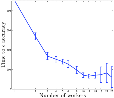
We simulate the cyclic delayed optimization algorithm (9) for the problem (17) for several choices of the number of workers and the number of samples computed at each worker. We summarize the results of our experiments in Figure 4. To generate the figure, we fix an (in this case, ), then measure the time it takes the stochastic algorithm (9) to output an such that . We perform each experiment ten times.
After computing the number of iterations required to achieve -accuracy, we convert the results to running time by assuming it takes one unit of time to compute the gradient of one term in the sum defining the objective (17). We also assume that it takes unit of time, i.e. , to communicate from one of the workers to the master, for the master to perform an update, and communicate back to one of the workers. In an node system where each worker computes samples of the gradient, the master receives an update every time units. A centralized algorithm computing samples of its gradient performs an update every time units. By multiplying the number of iterations to -optimality by for the distributed method and by for the centralized, we can estimate the amount of time it takes each algorithm to achieve an -accurate solution.
We now turn to discussing Figure 4. The delayed update (9) enjoys speedup (the ratio of time to -accuracy for an -node system versus the centralized procedure) nearly linear in the number of worker machines until or so. Since we use the stepsize choice , which yields the predicted convergence rate given by Corollary 2, the term in the convergence rate presumably becomes non-negligible for larger . This expands on earlier experimental work with a similar method [LSZ09], which experimentally demonstrated linear speedup for small values of , but did not investigate larger network sizes. Roughly, as predicted by our theory, for non-asymptotic regimes the cost of communication and delays due to using nodes mitigate some of the benefits of parallelization. Nevertheless, as our analysis shows, allowing delayed and asynchronous updates still gives significant performance improvements.
6 Delayed Updates for Smooth Optimization
In this section, we prove Theorems 1 and 2. We collect in Appendix A a few technical results relevant to our proof; we will refer to results therein without comment. Before proving either theorem, we state the lemma that is the key to our argument. Lemma 4 shows that certain gradient-differencing terms are essentially of second order. As a consequence, when we combine the results of the lemma with Lemma 7, which bounds , the gradient differencing terms become for step size choice , or for .
Lemma 4.
Proof The proof follows by using a few Bregman divergence identities to rewrite the left hand side of the above equations, then recognizing that the result is close to a telescoping sum. Recalling the definition of a Bregman divergence (2), we note the following well-known four term equality, a consequence of straightforward algebra: for any ,
| (18) |
Using the equality (18), we see that
| (19) | ||||
To make (19) useful, we note that the Lipschitz continuity of implies
so that recalling the definition of (2) we have
In particular, using the non-negativity of , we can replace (19) with the bound
Summing the inequality, we see that
| (20) |
To bound the first Bregman divergence term, we recall that by Assumption C and the strong convexity of , , and hence the optimality of implies
This gives the first bound of the lemma. For the second bound, using convexity, we see that
so by taking expectations we have . Since is non-increasing (by the definition of the update scheme) we see that the sum (20) is further bounded by as desired. ∎
6.1 Proof of Theorem 1
The essential idea in this proof is to use convexity and smoothness to bound , then use the sequence , which decreases the stepsize , to cancel variance terms. To begin, we define the error
where for some . Note that does not have zero expectation, as there is a time delay.
By using the convexity of and then the -Lipschitz continuity of , for any , we have
so that
Now, by applying Lemma 5 in Appendix A and the definition of the update (9), we see that
which implies
| (21) | ||||
To get the bound (21), we substituted and then used the fact that is strongly convex, so . By summing the bound (21), we have the following non-probabilistic inequality:
| (22) | ||||
since and minimizes . What remains is to control the summed terms in the bound (22). We can do this simply using the second part of Lemma 4. Indeed, we have
| (23) | ||||
We can apply Lemma 4 to the first term in (23) by bounding with Lemma 7. Since , Lemma 7 with implies . As a consequence,
What remains, then, is to bound the stochastic (second) term in (23). This is straightforward, though:
by the Fenchel-Young inequality applied to the conjugate pair and . In addition, is independent of given the sigma-field containing , since is a function of gradients to time , so the first term has zero expectation. Also recall that is bounded by by assumption. Combining the above two bounds into (23), we see that
| (24) | ||||
6.2 Proof of Theorem 2
The proof of Theorem 2 is similar to that of Theorem 1, so we will be somewhat terse. We define the error , identically as in the earlier proof, and begin as we did in the proof of Theorem 1. Recall that
| (25) |
Applying the first-order optimality condition to the definition of (5), we get
for all . In particular, we have
Applying the above to the inequality (25), we see that
| (26) | ||||
where for the last inequality, we use the fact that , by the strong convexity of , and that . By summing the inequality (26), we have
| (27) |
Comparing the bound (27) with the earlier bound for the dual averaging algorithms (22), we see that the only essential difference is the terms. The compactness assumption guarantees that , however, so
The remainder of the proof uses Lemmas 7 and 4 completely identically to the proof of Theorem 1.
6.3 Proof of Corollary 1
We prove this result only for the mirror descent algorithm (10), as the proof for the dual-averaging-based algorithm (9) is similar. We define the error at time to be , and observe that we only need to control the second term involving in the bound (26) differently. Expanding the error terms above and using Fenchel’s inequality as in the proofs of Theorems 1 and 2, we have
Now we note that conditioned on the delay , we have
Consequently we apply Lemma 4 (specifically, following the bounds (19) and (20)) and find
The sum of terms telescopes, leaving only terms not received by the gradient procedure within iterations, and we can use for all to derive the further bound
| (28) |
To control the quantity (28), all we need is to bound the expected cardinality of the set . Using Chebyshev’s inequality and standard expectation bounds, we have
where the last inequality comes from our assumption that . As in Lemma 4, we have , which yields
We can control the remaining terms as in the proofs of Theorems 1 and 2.
7 Proof of Theorem 3
The proof of Theorem 3 is not too difficult given our previous work—all we need to do is redefine the error and use to control the variance terms that arise. To that end, we define the gradient error terms that we must control. In this proof, we set
| (29) |
where is the gradient of node computed at the parameter and is the delay associated with node .
Using Assumption B as in the proofs of previous theorems, then applying Lemma 5, we have
We telescope as in the proofs of Theorems 1 and 2, canceling with the divergence terms to see that
| (30) | ||||
This is exactly as in the non-probabilistic bound (22) from the proof of Theorem 1, but the definition (29) of the error here is different.
What remains is to control the error term in (30). Writing the terms out, we have
| (31) |
Bounding the first term above is simple via Lemma 4: as in the proof of Theorem 1 earlier, we have
We use the same technique as the proof of Theorem 1 to bound the second term from (31). Indeed, the Fenchel-Young inequality gives
By assumption, given the information at worker at time , is independent of , so the first term has zero expectation. More formally, this happens because is a function of gradients from each of the nodes and hence the expectation of the first term conditioned on is 0. The last term is canceled by the Bregman divergence terms in (30), so combining the bound (31) with the above two paragraphs yields
8 Conclusion and Discussion
In this paper, we have studied dual averaging and mirror descent algorithms for smooth and non-smooth stochastic optimization in delayed settings, showing applications of our results to distributed optimization. We showed that for smooth problems, we can preserve the performance benefits of parallelization over centralized stochastic optimization even when we relax synchronization requirements. Specifically, we presented methods that take advantage of distributed computational resources and are robust to node failures, communication latency, and node slowdowns. In addition, by distributing computation for stochastic optimization problems, we were able to exploit asynchronous processing without incurring any asymptotic penalty due to the delays incurred. In addition, though we omit these results for brevity, it is possible to extend all of our expected convergence results to guarantees with high-probability.
Acknowledgments
In performing this research, AA was supported by a Microsoft Research Fellowship, and JCD was supported by the National Defense Science and Engineering Graduate Fellowship (NDSEG) Program. We are very grateful to Ofer Dekel, Ran Gilad-Bachrach, Ohad Shamir, and Lin Xiao for illuminating conversations on distributed stochastic optimization and communication of their proof of the bound (8). We would also like to thank Yoram Singer for reading a draft of this manuscript and giving useful feedback.
Appendix A Technical Results about Proximal Functions
In this section, we collect several useful results about proximal functions and continuity properties of the solutions of proximal operators. We give proofs of all uncited results in Appendix B. We begin with results useful for the dual-averaging updates (4) and (9).
We define the proximal dual function
| (32) |
Since , it is clear that . Further by strong convexity of , we have that is -Lipschitz continuous [Nes09, HUL96b, Chapter X], that is, for the norm with respect to which is strongly convex and its associated dual norm ,
| (33) |
We will find one more result about solutions to the dual averaging update useful. This result has essentially been proven in many contexts [Nes09, Tse08, DGBSX10a].
Lemma 5.
Let minimize for all . Then for any ,
Now we turn to describing properties of the mirror-descent step (5), which we will also use frequently. The lemma allows us to bound differences between and for the mirror-descent family of algorithms.
Lemma 6.
Let minimize over . Then .
The last technical lemma we give explicitly bounds the differences between and , for some , by using the above continuity lemmas.
Appendix B Proofs of Proximal Operator Properties
Proof of Lemma 6 The inequality is clear when , so assume that . Since minimizes , the first order conditions for optimality imply
for any . Thus we can choose and see that
where the last inequality follows from the strong convexity of .
Using Hölder’s inequality gives that , and dividing by completes the proof.
∎
Proof of Lemma 7 We first show the lemma for the dual-averaging updates. Recall that and is -Lipschitz continuous. Using the triangle inequality,
| (34) |
It is easy to check that for ,
By convexity of , we can bound :
since by assumption. Thus, bound (34) gives
where we use Cauchy-Schwarz inequality in the first step. Since , the last term is clearly bounded by .
To get the slightly tighter bound on the first moment in the statement of the lemma, simply use the triangle inequality from the bound (34) and that .
The proof for the mirror-descent family of updates is similar. We focus on non-delayed update (5), as the other updates simply modify the indexing of below. We know from Lemma 6 and the triangle inequality that
Squaring the above bound, taking expectations, and recalling that is non-increasing, we see
by Hölder’s inequality. Substituting the appropriate value for
completes the proof.
∎
Appendix C Error in [LSZ09]
Langford et al. [LSZ09], in Lemma 1 of their paper, state an upper bound on that is essential to the proofs of all of their results. However, the lemma only holds as an equality for unconstrained optimization (i.e. when the set ); in the presence of constraints, it fails to hold (even as an upper bound). To see why, we consider a simple one-dimensional example with , , and we evaluate both sides of their lemma with and . The left hand side of their bound evaluates to , while the right hand side is , and the inequality claimed in the lemma fails. The proofs of their main theorems rely on the application of their Lemma 1 with equality, restricting those results only to unconstrained optimization. However, the results also require boundedness of the gradients over all of as well as boundedness of the distance between the iterates . Few convex functions have bounded gradients over all of ; and without constraints the iterates are seldom bounded for all iterations .
References
- [ABRW10] A. Agarwal, P. Bartlett, P. Ravikumar, and M. Wainwright, Information-theoretic lower bounds on the oracle complexity of convex optimization, Submitted to IEEE Transactions on Information Theory, URL http://arxiv.org/abs/1009.0571, 2010.
- [Ber73] D. P. Bertsekas, Stochastic optimization problems with nondifferentiable cost functionals, Journal of Optimization Theory and Applications 12 (1973), no. 2, 218–231.
- [Bre67] L. M. Bregman, The relaxation method of finding the common point of convex sets and its application to the solution of problems in convex programming, USSR Computational Mathematics and Mathematical Physics 7 (1967), 200–217.
- [BT89] D. P. Bertsekas and J. N. Tsitsiklis, Parallel and distributed computation: numerical methods, Prentice-Hall, Inc., 1989.
- [BT03] A. Beck and M. Teboulle, Mirror descent and nonlinear projected subgradient methods for convex optimization, Operations Research Letters 31 (2003), 167–175.
- [DAW10] J. Duchi, A. Agarwal, and M. Wainwright, Dual averaging for distributed optimization: convergence analysis and network scaling, URL http://arxiv.org/abs/1005.2012, 2010.
- [DGBSX10a] O. Dekel, R. Gilad-Bachrach, O. Shamir, and L. Xiao, Optimal distributed online prediction using mini-batches, URL http://arxiv.org/abs/1012.1367, 2010.
- [DGBSX10b] , Robust distributed online prediction, URL http://arxiv.org/abs/1012.1370, 2010.
- [HTF01] T. Hastie, R. Tibshirani, and J. Friedman, The elements of statistical learning, Springer, 2001.
- [HUL96a] J. Hiriart-Urruty and C. Lemaréchal, Convex Analysis and Minimization Algorithms I, Springer, 1996.
- [HUL96b] , Convex Analysis and Minimization Algorithms II, Springer, 1996.
- [JNT08] A. Juditsky, A. Nemirovski, and C. Tauvel, Solving variational inequalities with the stochastic mirror-prox algorithm, URL http://arxiv.org/abs/0809.0815, 2008.
- [JRJ09] B. Johansson, M. Rabi, and M. Johansson, A randomized incremental subgradient method for distributed optimization in networked systems, SIAM Journal on Optimization 20 (2009), no. 3, 1157–1170.
- [Lan10] G. Lan, An optimal method for stochastic composite optimization, Mathematical Programming Series A (2010), Online first, to appear. URL http://www.ise.ufl.edu/glan/papers/OPT_SA4.pdf.
- [LMP01] J. Lafferty, A. McCallum, and F. Pereira, Conditional random fields: Probabilistic models for segmenting and labeling sequence data, Proceedings of the Eightneenth International Conference on Machine Learning, 2001, pp. 282–289.
- [LSZ09] J. Langford, A. Smola, and M. Zinkevich, Slow learners are fast, Advances in Neural Information Processing Systems 22, 2009, pp. 2331–2339.
- [LYRL04] D. Lewis, Y. Yang, T. Rose, and F. Li, RCV1: A new benchmark collection for text categorization research, Journal of Machine Learning Research 5 (2004), 361–397.
- [NBB01] A. Nedić, D.P. Bertsekas, and V.S. Borkar, Distributed asynchronous incremental subgradient methods, Inherently Parallel Algorithms in Feasibility and Optimization and their Applications (D. Butnariu, Y. Censor, and S. Reich, eds.), Studies in Computational Mathematics, vol. 8, Elsevier, 2001, pp. 381–407.
- [Nes09] Y. Nesterov, Primal-dual subgradient methods for convex problems, Mathematical Programming A 120 (2009), no. 1, 261–283.
- [NJLS09] A. Nemirovski, A. Juditsky, G. Lan, and A. Shapiro, Robust stochastic approximation approach to stochastic programming, SIAM Journal on Optimization 19 (2009), no. 4, 1574–1609.
- [NO09] A. Nedić and A. Ozdaglar, Distributed subgradient methods for multi-agent optimization, IEEE Transactions on Automatic Control 54 (2009), 48–61.
- [NY83] A. Nemirovski and D. Yudin, Problem complexity and method efficiency in optimization, Wiley, New York, 1983.
- [Pol87] B. T. Polyak, Introduction to optimization, Optimization Software, Inc., 1987.
- [RM51] H. Robbins and S. Monro, A stochastic approximation method, Annals of Mathematical Statistics 22 (1951), 400–407.
- [RNV10] S. S. Ram, A. Nedić, and V. V. Veeravalli, Distributed stochastic subgradient projection algorithms for convex optimization, Journal of Optimization Theory and Applications 147 (2010), no. 3, 516–545.
- [Tse08] P. Tseng, On accelerated proximal gradient methods for convex-concave optimization, Tech. report, Department of Mathematics, University of Washington, 2008.
- [Tsi84] J. Tsitsiklis, Problems in decentralized decision making and computation, Ph.D. thesis, Massachusetts Institute of Technology, 1984.
- [Xia10] L. Xiao, Dual averaging methods for regularized stochastic learning and online optimization, Journal of Machine Learning Research 11 (2010), 2543–2596.