Galaxy growth by merging in the nearby universe
Abstract
We measure the mass growth rate by merging for a wide range of galaxy types. We present the small-scale () projected cross-correlation functions of galaxy subsamples from the spectroscopic sample of the NYU VAGC ( galaxies of redshifts ) with galaxy subsamples from the SDSS imaging ( galaxies). We use smooth fits to de-project the two-dimensional functions to obtain smooth three-dimensional real-space cross-correlation functions for each of several spectroscopic subsamples with each of several imaging subsamples. Because close pairs are expected to merge, the three-space functions and dynamical evolution time estimates provide galaxy accretion rates. We find that the accretion onto massive blue galaxies and onto red galaxies is dominated by red companions, and that onto small-mass blue galaxies, red and blue galaxies make comparable contributions. We integrate over all types of companions and find that at fixed stellar mass, the total fractional accretion rates onto red galaxies ( ) is greater than that onto blue galaxies ( ). These rates are almost certainly over-estimates because we have assumed that all close pairs merge as quickly as the merger time that we used. One conclusion of this work is that if the total growth of red galaxies from to is mainly due to merging, the merger rates must have been higher in the past.
1 INTRODUCTION
The galaxy mergers may play an important role in the evolution of the galaxies. In the color-magnitude space, galaxies are separated into two distinct regions: (1) the ‘red sequence’: the ‘early-type’, red galaxies ; (2) the ‘blue cloud’ or ‘blue sequence’: the ‘late-type’, blue galaxies with strong ongoing star formation (Strateva et al., 2001; Blanton et al., 2003b). Some recent studies in the high-redshift () universe find that the early-type galaxy population is growing over time (Bell et al., 2004; Willmer et al., 2006; Blanton, 2006; Brown et al., 2007; Faber et al., 2007; Zhu et al., 2011), which is also found at very high () redshift (Daddi et al., 2005; Trujillo et al., 2007; Longhetti et al., 2007; Toft et al., 2007; Conselice et al., 2007; Cimatti et al., 2008; van Dokkum et al., 2008; Saracco et al., 2009). In numerical simulations, some studies show us that major mergers of intermediate-stellar-mass late-type galaxies maybe play an important role in the growth of the intermediate-stellar-mass early type galaxies (Barnes & Hernquist, 1996; Naab & Burkert, 2003). However, the massive early type galaxies may grow in a different way (Naab & Burkert, 2003). Some recent studies show us that ‘dry mergers’ - the mergers between early-type galaxies - might play an important role in the growth of massive early-type galaxies (Bell et al., 2006b; van Dokkum, 2005; Masjedi et al., 2008).
There are a lot of studies that estimate the merger rate among galaxies. These studies can be separated into two general categories. The studies in the first category count the ‘pre-merger’ close pairs and convert the ‘pre-merger’ pairs to a merger rate (e.g., Zepf & Koo, 1989; Carlberg et al., 1994, 2000; Carlberg et al., 2000; Patton et al., 1997, 2000; van Dokkum et al., 1999; Lin et al., 2004; Bell et al., 2005; Bell et al., 2006a; Kartaltepe et al., 2007; Masjedi et al., 2006, 2008; Patton & Atfield, 2008; Kitzbichler & White, 2008; Bundy et al., 2009; De Propris et al., 2007; Lin et al., 2008; de Ravel et al., 2009; De Propris et al., 2010; Robaina et al., 2010). The studies in the second category count the ‘post-merger’ galaxies which have recently experienced at least one merger event. These ‘post-merger’ galaxies are chosen by some observable special properties caused by merging. An example might be by star formation indicators of ‘post-merger’ galaxies (Quintero et al., 2004) or by morphological signatures caused by merger events (Abraham et al., 1996; Conselice et al., 2003; van Dokkum, 2005; Lotz et al., 2006; De Propris et al., 2007; Lotz et al., 2008; Conselice et al., 2009).
Our work builds on the earlier works of Masjedi et al. (2006, 2008), which have found previously that luminous red galaxies (LRGs) are growing on average by less than 2 from merger activity at redshifts (Masjedi et al., 2008). In this paper, we consider both red and blue galaxies. We use the previous technique for measuring the close pairs (Masjedi et al., 2008) on NYU VAGC Spectroscopic Sample and SDSS Imaging Sample, and extend this type of analysis beyond luminous red galaxies (LRGs) to a wide range of galaxies in both stellar mass and color.
The primary uncertainty in turning a deprojected three-dimensional cross-correlation function at small scales into a merger rate is in estimating the mean time for two galaxies to merge as a function of stellar mass and separation. There are different estimates of merger timescale: free-fall time, orbital time, and dynamical friction time (e.g., Binney & Tremaine 1987; Boylan-Kolchin & Ma 2007; Conroy et al. 2007; Kitzbichler & White 2008; Bundy et al. 2009; Lotz et al. 2010). In this paper, we will use an approximation to the two kinds of merger times under the assumption of Kitzbichler & White (2008) and Binney & Tremaine (1987) as our standard estimate. Both of these times are likely to be an under-estimate of the mean merger time, because some close pairs will not merge at all. Any under-estimate of the merger time leads to an over-estimate of the growth rate.
Throughout this paper, all magnitudes are AB, all apparent magnitudes are model Mag, all masses are stellar masses (in units of ), all velocities are in units of , all radii of galaxies are which contain percent of the Petrosian flux (Blanton et al., 2003b; Blanton & Moustakas, 2009), and all volumes and distances are comoving, calculated for a cosmological world model with and Hubble constant .
2 DATA
We use the NYU Value-Added Galaxy Catalog (VAGC) V7.2 data (Blanton et al., 2005), which is built from SDSS data, as our source of spectroscopic data. We use all the SDSS imaging data as our source for cross-correlation samples. The SDSS is a survey of about square degrees (Fukugita et al., 1996; Gunn et al., 1998; Gunn et al., 2006; York et al., 1999; York & SDSS Collaboration, 2001; Stoughton et al., 2002; Abazajian et al., 2003, 2004).
2.1 Spectroscopic Subsample
Our spectroscopic sample is drawn from NYU VAGC V7.2 data. We removed galaxies with apparent magnitudes , because SDSS photometric catalog missed many luminous galaxies nearby (Zhu et al., 2010). Our spectroscopic sample contains about main galaxies, of which about SDSS Main Samples galaxies (Strauss et al., 2002) are in the redshift range (see Figure 1) with apparent magnitudes . We cut the redshift at , because we want to avoid all quasars, and we cut the redshift at , because we want to avoid all stars. We use the code sdss_kcorrect (Blanton & Roweis, 2007) to calculate the -corrected absolute magnitude at and stellar mass for each. We cut this sample into 10 subsamples by stellar mass and make sure that in each subsamples the number of galaxies is the same. After that, we cut them into red and blue using the cut (Hogg et al., 2004):
| (1) |
where is the stellar mass. These cut the spectroscopic sample into 20 spectroscopic subsamples; we call these subsamples (see Figure 2). For the red spectroscopic subsamples, we name the smallest stellar-mass subsample ‘red0’, then name the second smallest stellar-mass subsample ‘red1’, and so on, so the largest stellar-mass subsample is named ‘red9’, and the same for the blue spectroscopic subsamples. Figures 3 and 4 show the number density of galaxies of the 18 spectroscopic subsamples as a function of redshift. The red0 and blue0 subsamples are low in number density, and highly affected by survey selection effects, so we do not use them further. We can see that blue8, blue9 and red9 appear to rise in number density with redshift, this is because we removed galaxies with apparent magnitudes .
The SDSS suffers from the ‘fiber collision’: the angular separation between any two spectroscopic targets must be larger than 55 arcsec. There are about percent of target galaxies which do not have redshifts because of this fiber collision. Using the counting-close-pairs technique of Masjedi et al. (2008), the fiber collision will not affect our pair counts directly under the approximation that the unmeasured galaxies and the measured galaxies are similar in cross-correlation with fainter galaxies.
Following the technique of Masjedi et al. (2008), we estimate the weight that accounts the spectroscopic incompleteness from fiber collisions effects, and the weight that accounts the spectroscopic incompleteness from all other selection effects in SDSS. For each galaxy in the spectroscopic subsample, we calculate by using a two-dimensional ‘FOF’ (friends-of-friends) grouping algorithm on our main galaxies targets with a 55-arcsec linking length:
| (2) |
Where is the total number of main galaxies targets in group , is the number of main galaxies with redshift measurement in group , and the group which contains galaxy , is called group . All because .
For each spectroscopic subsample , we create a random spectroscopic subsample which is 10 times large as . For each galaxy in , we created 10 galaxies with the exactly same redshift but angular position taken from the two-dimensional random sample. Thus, we create a large random spectroscopic subsample which match the redshift distribution of , and is isotropic within the SDSS survey region.
The SDSS survey region is separated into small unique region ‘sector’. For each random point in :
| (3) |
Where is the fraction of main galaxy targets for which a classification was obtained in the object’s sector (in our NYU-VAGC spectroscopic sample, the average is ).
Our correction of fiber collisions is: we weight the target in spectroscopic subsample as and weight the target in random spectroscopic subsample as . From the previous work (Masjedi et al., 2006), we know that this correction will improve in the spectroscopic incompleteness due to fiber collisions at very small separations (). In Section 4.1, we will compare our result with the result of Zehavi et al. (2010), and will show that our result with this correction of fiber collisions fits better than the result without this correction of fiber collisions.
For each spectroscopic sample ‘s’ ( or ), in which there are spectroscopic galaxies, we divide it into the 50 bins by lines of constant dec, so that there are spectroscopic galaxies in each bin. Then we resample them into 50 leave-one-out resampling samples, so that there are spectroscopic galaxies in each sample. We call them the ‘50 resampling samples’, with which we can calculate our jackknife resampling covariance matrix.
2.2 Imaging Subsamples
For our imaging data, we use a sample drawn from the full SDSS imaging catalog in which there are about galaxies. We include from the SDSS imaging sample only galaxies with apparent magnitude , and apparent color , see Figures 5 and 6. We removed galaxies with apparent magnitudes for the same reason with our spectroscopic sample. We also removed galaxies with apparent magnitudes , because these galaxies are not well observed and their observed number density is much lower than their real number density. Please note that this cut will affect our minor merger near mass ratio . Similar to the spectroscopic sample, we create a random imaging sample as large as possible. The angular positions of galaxies in are taken from the two-dimensional random sample. So is isotropic within the SDSS survey region.
2.3 Grid Method -corrections for galaxies from the imaging sample
We also need to compute the stellar mass of galaxies in the imaging subsamples in order to determine the mass ratio, so we want to -correct galaxies in the imaging subsamples. However, we cannot -correct individual galaxies in the imaging subsamples once and for all, because we do not have spectroscopic redshifts for them. Each time we consider a pair of galaxies, one from the spectroscopic subsample and one from the imaging subsample, we assign the spectroscopic redshift to the galaxy from the imaging sample. This allows us to calculate for each galaxy from the imaging sample in each spectroscopic–imaging pair a temporary -corrected stellar mass and [] color for the purposes of that pair. We discard these values and compute new ones when the galaxy from the imaging sample is used in another pair with another galaxy from the spectroscopic sample.
To save time, we take galaxies from the NYU VAGC spectroscopic sample as representative of all galaxy types, and apply the code sdss_kcorrect on the galaxies from a grid named ‘B’ of observed -band magnitude (0.5 mag per bin), [] color (0.1 mag per bin), and redshifts between 0.03 and 0.15 (0.0002 per bin). We saved the mean -corrected stellar mass and [] color in a grid of observed -band magnitude, [] color, and redshift, also save the mean redshift , mean and mean [] color, Thereafter we estimated the -corrected stellar mass and [] color for a galaxy G in grid B, and the [] color of galaxy G is between [] color of grid B and [] color of grid C which is next to grid B (that means and are the same, and and are the same):
| (4) |
| (5) |
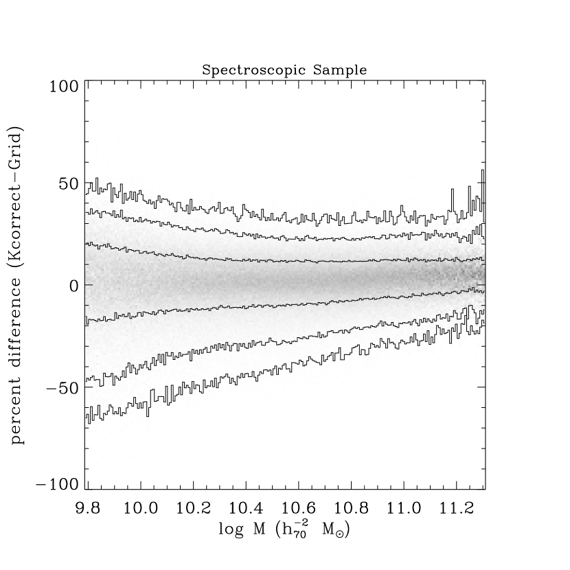
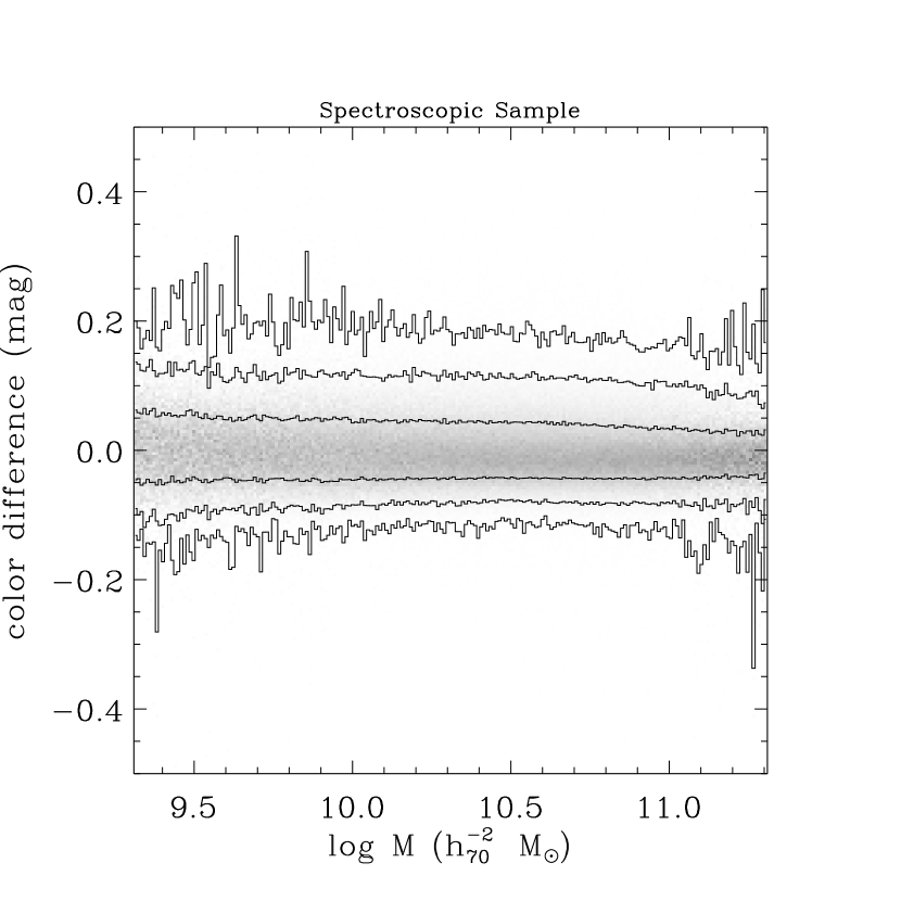
where is the luminosity distance calculated from redshift, and galaxy G is in grid B, so the difference between and is small, similarly, the difference is small between and , and , [] and []. because of these small differences, the equations (4) and (5) can be used. This speeds up the -correction procedure immensely and only introduces a 12-percent one-sigma error for each galaxy and there is little bias (see Figure 7), so only introduces percent-level errors in the results. We call this ‘Grid Method’ hereafter.
For grids with observed -band magnitude , we cannot get the mean stellar mass and [] color directly, because there are no galaxies from the spectroscopic sample at observed -band magnitude . In order to estimate the color and stellar mass of the galaxies in grid A with mean observed -band magnitude , we find the grid point B that has the nearest mean observed -band magnitude () and has the same observed [] color and the same redshift, also there are at least 10 galaxies from the spectroscopic sample in grid B. Then we estimate and color of galaxy G in grid A using the equation (4) and (5). If we cannot find a grid B satisfying the conditions, we will leave all the galaxies in grid A empty.
2.4 Velocities for merger rate estimates
In this Section, we will estimate the average orbital velocity which will be used to estimate the merger time in Section 3.4. Please note that this approximation will induce a large error in the estimate of merger time, because we assume that all close pairs merge under the following orbital velocity which is not true for close pairs in high velocity-dispersion.
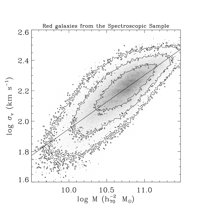
The average orbital velocity for a galaxy from the imaging sample around a more massive red galaxy from the spectroscopic subsample with average velocity dispersion is very roughly times the velocity dispersion, here we have included the factor of 1.5 to be conservative (Masjedi et al., 2008). We estimate the with Faber-Jackson relation:
| (6) |
where is the mean stellar mass of the red galaxies from spectroscopic subsample . We performed a linear fit to the data to obtain and (Figure 9). Please note that the method above will induce a small enough error () into our final result.
We estimate the average orbital velocity for a galaxy from the imaging sample around a more massive blue galaxy from the spectroscopic subsample with the Tully-Fisher relation:
| (7) |
where is the mean I-band luminosity of the blue galaxies from spectroscopic subsample , calculated from , where is the stellar mass of the galaxy and is the I-band mass-to-light ratio of the galaxy calculated from the code sdss_kcorrect. We used for this relationship and (Courteau et al., 2007).
Table 1 provides this information for all 20 spectroscopic subsamples.
3 Method
For each spectroscopic subsample , we cut the imaging sample into 16 subsamples by stellar mass: , where is the stellar mass of a galaxy from the imaging sample, calculated by the Grid Method using the redshift of the spectroscopic galaxy, and is the mean stellar mass of the galaxies from spectroscopic subsample , and is an integer , that means a mass ratio of to is covered. After that, we cut them into red and blue using equation (1) by color calculated by Grid Method. For each spectroscopic subsample , these cut the imaging sample into 32 imaging subsamples .
In this section, we will show our method to estimate the merger rate between galaxies in spectroscopic subsample and galaxies in imaging subsample : (1) we estimate the projected two-dimensional cross-correlation function as a function of tangential projected separation ; (2) we de-project the smooth fit for the cross-correlation function to obtain the three-dimensional real-space cross-correlation function as a function of real-space separation ; (3) we estimate the merger rate using and our two kinds of merger times (Binney & Tremaine, 1987; Kitzbichler & White, 2008). In addition, we will also discuss our method of photometry correction.
3.1 Projected cross-correlation function
To estimate the between spectroscopic subsample and imaging subsample , we can integrate along the line of sight (e.g., Davis & Peebles 1983):
| (8) |
This integral is dominated by scales .
Using the previous approach (Masjedi et al., 2006, 2008), we estimate not but , where is the average comoving three-dimensional stellar mass density of the imaging subsample :
| (9) |
Where and represent the spectroscopic and imaging data subsamples, and and represent the spectroscopic and imaging random subsamples. Similar to the previous method (Masjedi et al., 2006, 2008), equation (9) measures the mass-weighted abundance of pairs () and subtracts the mean background level (). This method has been well tested in Masjedi et al. (2006).
In detail, the factors are defined as follows:
| (10) |
where the top sum counts the weighted pairs of galaxies from and separated by tangential projected distance , and the bottom sum is over galaxies from . This factor is dimensionless.
| (11) |
where the top sum counts the weighted pairs of galaxies from and separated by tangential projected distance . In the bottom, is the inverse square of the transverse comoving distance (Hogg, 1999) to galaxy from , and is calculated by , where is the two-dimensional number density of per solid angle, and
| (12) |
where is the mean stellar mass of galaxies from the imaging subsample , and is an integer . Then represents the average stellar mass of galaxies in per unit comoving area around each galaxy from . This factor has dimensions of comoving area divided by stellar mass.
| (13) |
this is similar to equation (10), but represents now the random catalog mentioned in Section 2.1. This factor is dimensionless.
| (14) |
this is similar to equation (11), but represents now the random catalog mentioned in Section 2.1. This factor has dimensions of comoving area divided by stellar mass.
For some experiments, we need to estimate , where is the average comoving three-dimensional number density of the imaging subsample . We estimate this by the following estimation:
| (15) |
For and , it is as the same as equation (10) and equation (13). For and :
| (16) |
this is similar to equation (11), but is the two-dimensional number density of the random imaging catalog per solid angle. This factor has dimensions of comoving area.
| (17) |
this is similar to equation (14). This factor has dimensions of comoving area.
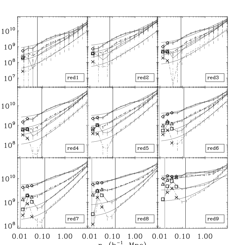
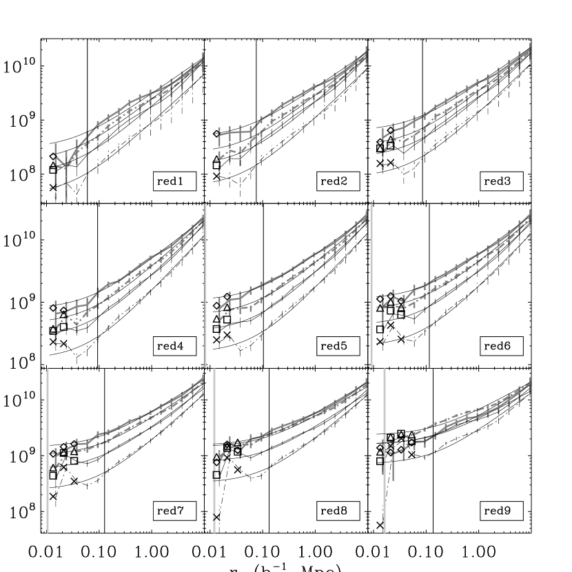
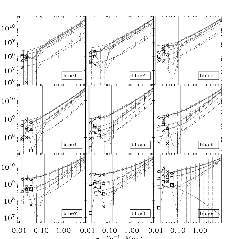
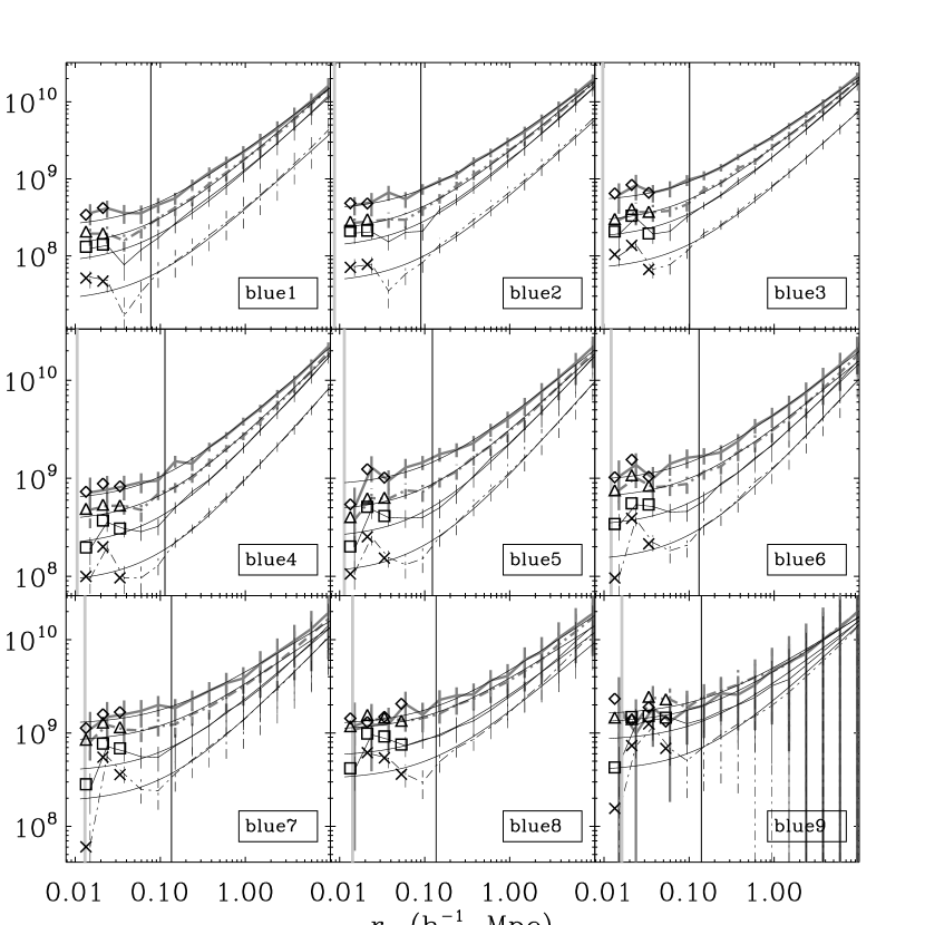
In range of our interest , we bin the spectroscopic-imaging pairs counting by the comoving projected separation of the pair where and is an integer . We have already discussed how to bin the spectroscopic sample and the imaging sample in Section 2. We have combined the 16 stellar mass bins into 4 to simplify the figures. Figures 10 through 13 show the results of our measurements of .
The uncertainties on the results shown in these figures are estimated using jackknife resampling covariance matrix with 50 resampling samples (see Section 2.1), please note that all the error bars in our graphs only come from the jackknife resampling covariance matrix (there are some other errors like the error of the color and stellar mass estimated by the Grid Method, and so on). On hundreds of kiloparsec scales, the error bars for each subsample are smallest. On smaller scales, the error bars become larger because of the ‘shot noise’: the smaller the separations, the fewer the pair counts. On larger scales (), the error bars become larger because there are more and more interlopers on larger scales which means that the background subtraction is more noisy.
Figures 10 through 13 show that is a complex function of . However, on very small scales - tens of kiloparsec scales, we assume that scales (something) like (Masjedi et al., 2006, 2008). We fit each set of data with the smooth model:
| (18) |
by minimizing
| (19) |
We choose for Figure 10 to Figure 13 (where is the median radii of the galaxies in the corresponding spectroscopic subsamples); then find the and that minimizes . Figures 10 through 13 show us these fits.
3.2 Photometry Correction
One important issue with all clustering measurements on small scales is possible photometric biases when measuring close pairs. This issue can directly lead to biased flux measurements (Masjedi et al., 2006) and biased color measurements for galaxies, and will indirectly affect stellar masses, k-corrections, etc. This can be due to poor photometry in crowded systems (Patton et al., 2011).
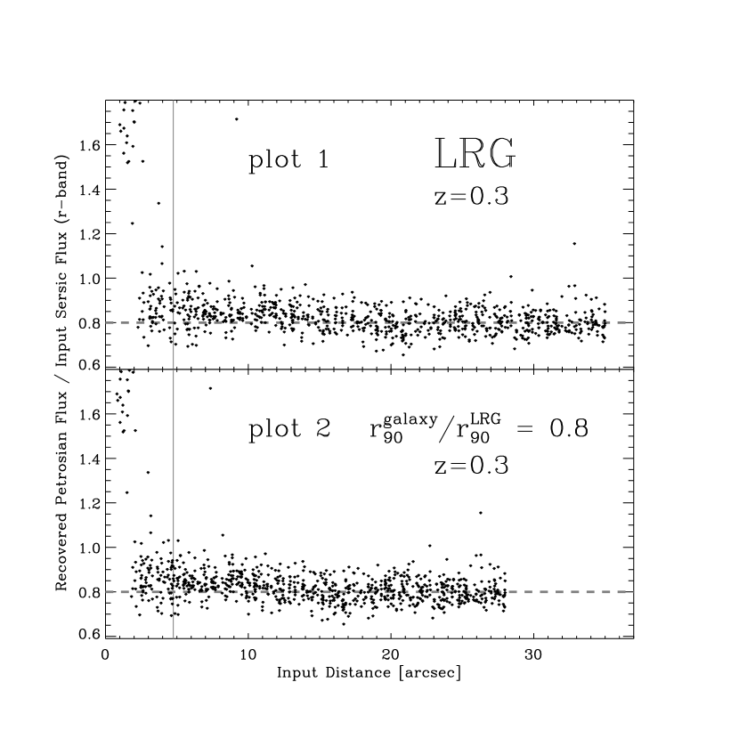
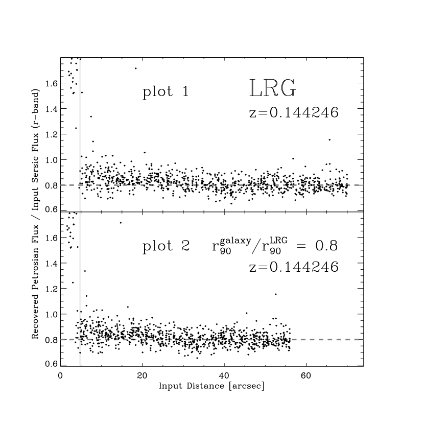
We build our method to correct photometric biases upon the photometry test of Masjedi et al. (2006). In Masjedi et al. (2006), they created fake images of pairs of identical galaxies with separations ranging from to . These galaxies represent passively evolving LRG galaxies observed at a redshift of with de Vaucouleurs profiles ( Srsic profiles). Then they placed one such galaxy pair onto RUN (which has a typical SDSS seeing of about ) of SDSS imaging. After inputting the known info into the mock galaxy images, they processed these images as raw SDSS images using the standard SDSS pipeline, PHOTO, to determine the effect of proximity of galaxies on their measured properties (see plot in Figure 14). At separations larger than , the Petrosian flux measures percent of the input Srsic flux, which is calculated by three sigma out-layer rejected average. In other words, the Petrosian flux only measures about percent of a galaxy’s light. We are interested in intermediate separations, (), in which the fraction of the recovered flux to input flux increases to percent. This increase is likely due to a double counting of the low level diffuse emission from the two galaxies which is being poorly deblended between the two objects.
For pairs of main galaxies, we study two different cases: one for galaxy pairs consisting of two identical galaxies and another with galaxies of different stellar mass. For Case 1, we consider a pair of identical main galaxies with radii of (at redshift ) than that of the LRGs at redshift (see plot and in Figure 16). We take the following two approximations: (1) If we consider a pair of identical main galaxies which are at the same redshift , then the only difference between this pair of main galaxies and the pair of LRGs (see plot in Figure 14) is that the angular radii of the main galaxies is smaller than that of LRGs by a factor of . So we compress the result of plot 1 in Figure 14 by a factor of (see plot in Figure 14 as an example) as the effect of proximity of a pair of identical main galaxies. (2) If we consider a pair of LRGs which are at a different redshift , then the only difference between this pair of LRGs and the pair of the LRGs at redshift (see plot in Figure 14) is that the angular radii of this pair of LRGs is larger than that of the LRGs at redshift by a factor of , where is the comoving distance from to us, and is the comoving distance from to us. So we stretch the result of plot 1 in Figure 14 by a factor of (see plot in Figure 15 as an example, and at redshift is nearly half of ) as the effect of proximity of a pair of LRGs at redshift . Combining the above two approximations, the final effect of proximity of a pair of identical main galaxies at a different redshift , will be stretched by a factor of (see plot 2 Figure 15 as an example). Using this method we correct the flux measurement of our sample on small scales of major merger between main galaxies and we assume that the correction of stellar mass is equal to that of flux. For Case 2, it is based on the above Case but involving the radii of the pair of galaxies ( and ) in our estimation. In plot of Figure 16, we take the third approximation: (3) The flux density from the left galaxy onto the right galaxy is a constant (this approximation lead to a small error comparing to the flux density from the galaxy A onto the galaxy B in plot of Figure 16). We mark the percent increase of flux from the other galaxy as , that of stellar mass as , radius of galaxy A as total flux as and stellar mass as . Then we get the following result:
| (20) |
In plot of Figure 16, we assume that the flux density from the galaxy A onto the galaxy B is equal to and the flux density from galaxy B onto galaxy A is equal to . We mark the percent increase of flux of galaxy B from the galaxy A as , that of stellar mass as , radius of galaxy B as total flux as , stellar mass as , and the percent increase of flux of galaxy A from the galaxy B as , that of stellar mass as . Then we get the following results:
| (21) |
| (22) |
| (23) |
Using this result we correct the flux and stellar mass measurements of our sample on small scales of minor merger between main galaxies.
Please note that our photometry correction is overestimated because of the above approximations (1) and (2). In approximations (1) and (2), we assume that the absolute angular scale does not matter; and the only change comes from the ratio of the absolute angular radii of the pair of galaxies to the absolute angular separation of the pair of galaxies. However, we know that absolute angular scale does matter: at the same ratio the larger the absolute angular is, the easier the deblending will be. So approximations (1) and (2) will contribute a few percent error in our final result of photometry correction.
After the above photometry correction, we reset our spectroscopic and imaging subsamples to recalculate the using the method in Section 3.1 (see the first and second data points in Figures 10 through 13). Please note that we also apply our photometry correction on the galaxies with no nearby companions, however these galaxies have zero weight in our pair-counting and will not affect our result, because there are no companions near these galaxies during counting pairs. In order to show our method of photometry correction is robust, we double our photometry correction and find that all the percentage difference between the result of our photometry correction and double our photometry correction is below percent for one data point. Then, this data point with percent change will only contribute a few percent error in our final result of the total fractional accretion rate after our fitting curve (see equation (18) and (19)). So, if we assume that the percent error of our photometry correction in flux is , the final effect onto the total fractional accretion rate is at most a few percent.
We use the above method to correct the photometric biases, and we find that our correction due to photometric biases is much smaller than that of Masjedi et al. (2006), because: (1) Main galaxies have smaller radii than LRGs, so it is easier to deblend a pair of main galaxies than a pair of LRGs. (2) Photometry correction of auto-correlation of Masjedi et al. (2006) is larger than that of our cross-correlation, this is because of the difference of the stellar mass cut of spectroscopic/imaging sample between us: for auto-correlation, the stellar mass cut of spectroscopic/imaging sample will be and , so after photometry correction, the only effect is that some spectroscopic (and imaging) galaxies near will be cut off from the spectroscopic (and imaging) sample which will decrease the pair-counting. However this is not the only effect on cross-correlation. For cross-correlation, the stellar mass cut of spectroscopic and imaging sample will be and , so after photometry correction, besides the above effect there is another effect that some spectroscopic and imaging galaxies which are a little bit above or will be counted into the spectroscopic/imaging sample from outside. This effect will increase the pair-counting. Combining the two effects above for cross-correlation, the final photometry correction for cross-correlation will be smaller than that for auto-correlation.
3.3 Three-dimensional statistics
The smooth fit to each projected correlation functions can be deprojected to get an estimate of the three-dimensional space correlation function by
| (24) |
(e.g., Davis & Peebles, 1983), where is a constant.
The mean total stellar mass of galaxies from a specific imaging subsample within a given small three-dimensional separation around each galaxy from spectroscopic subsample is:
| (25) |
At small scales, , so:
| (26) |
From we can see that we do not need to measure and separately.
At very small scale ():
| (27) |
Similarly, the average number of galaxies from a specific imaging subsample within a given small three-dimensional separation per galaxy from spectroscopic subsample at very small scale () is:
| (28) |
3.4 Merger rate
We can estimate the merger rate of galaxies from sample into galaxies from sample per spectroscopic galaxy per unit time by:
| (29) |
The mean fractional stellar-mass accretion rate of galaxies from spectroscopic subsample from merging with galaxies from imaging subsample per unit time is:
| (30) |
In principle, all merger rate estimates depend on the radius inside of which we have counted close pairs. However in this work, we are interested in the instant merger rate estimates, which means that we are interested in the range of , and this range can be reached using our fit lines. Another reason why we use our fit lines instead of using the data points at very small scales, is that the error bars due to the shot noise for each subsample are very large. From these fit lines in Figures 10 through 13 we know, over the range of interest () scales like , scales like , and scale (something) like . Similarly, both of the time-scales ( and ) scale like . For this reason, at the above merger and accretion rates do not depend strongly on .
In this work, we use these two merger time estimates: from Binney & Tremaine (1987) and from Kitzbichler & White (2008). Both of them depend on the orbital merger time :
| (31) |
Where is the average orbital velocity for a galaxy from the imaging sample orbiting a more massive red galaxy from the spectroscopic sample with velocity dispersion , see equation (6). Similarly, the orbital merger time for a galaxy from the imaging sample merged into a more massive blue galaxy from the spectroscopic subsample is
| (32) |
Where is the average orbital velocity for a galaxy from the imaging sample around a more massive blue galaxy from the spectroscopic sample, see equation (6).
For the assumption of from Kitzbichler & White (2008), the approximation becomes
| (33) |
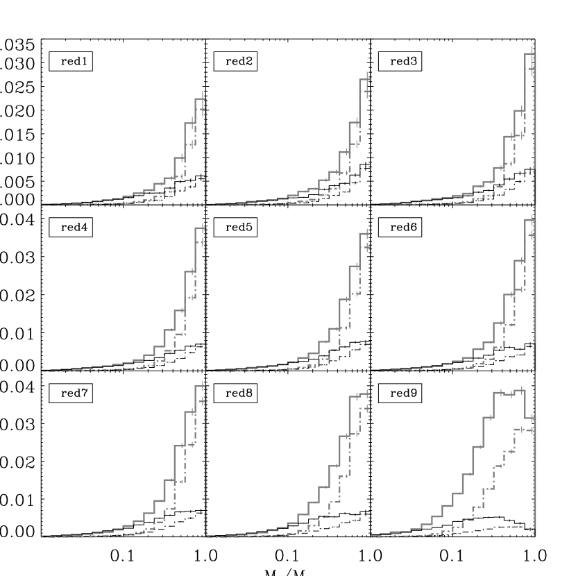
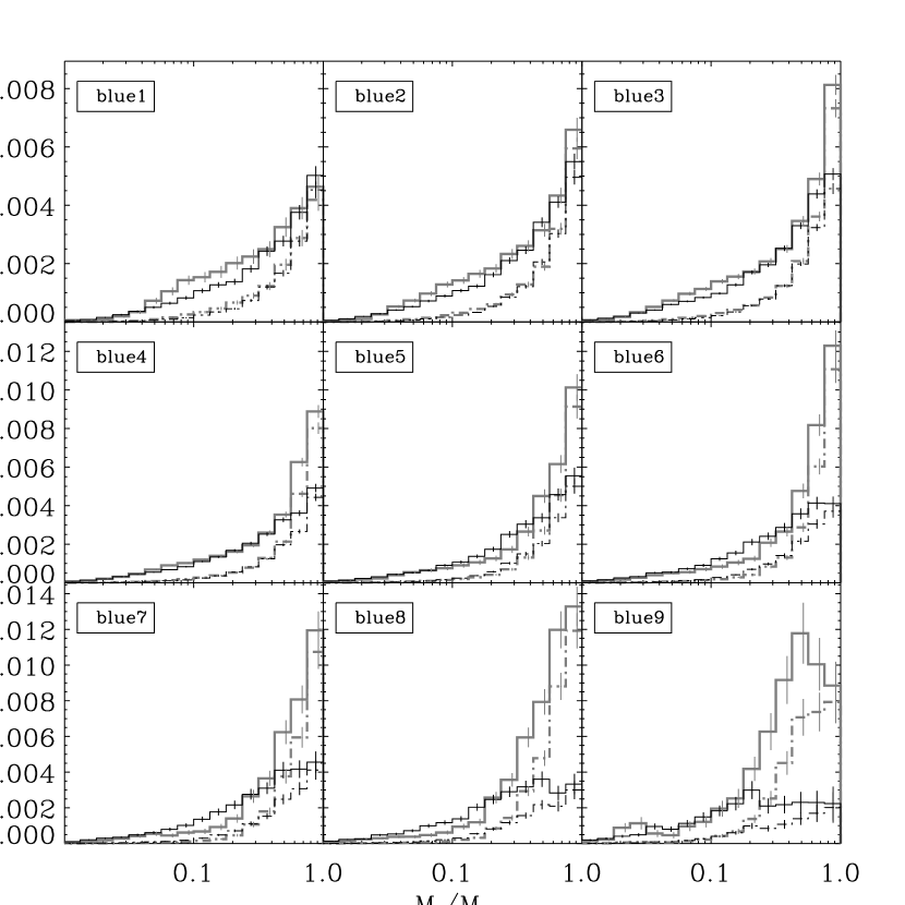
where we assume . The solid lines in Figures 17 and 18 as a function of the mass ratio show the merger rate under assumption of Kitzbichler & White (2008). The total fractional accretion rate is the area under each curve.
For the assumption of from Binney & Tremaine (1987), is longer than the rbital merger time by a factor roughly equal to the ratio of the stellar masses (Binney & Tremaine, 1987; Masjedi et al., 2008):
| (34) |
where we assumed . The dashed lines in Figures 17 and 18 as a function of the mass ratio show the merger rate under assumption of all possible mergers taking place within one dynamical friction time (Binney & Tremaine, 1987; Masjedi et al., 2008), and the total fractional accretion rate is the area under the curves.
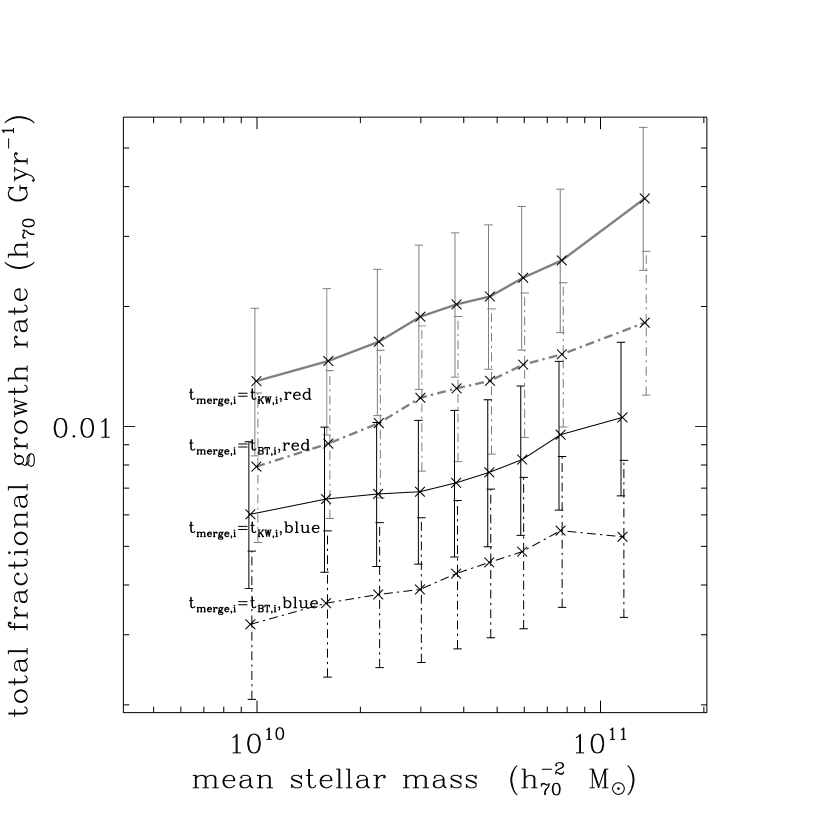
We integrate the mass accretion rate from mergers over all imaging subsamples and find the total fractional accretion rate () of all the main galaxies. This is shown with solid lines (for ) and dashed lines (for ) in Figure 19. Please note that the errors from merger time are shown in this figure.
Table 2 shows the total fractional accretion rates of all the 20 spectroscopic subsamples for both the assumption of and the assumption of .
4 Comparison to Previous Work
4.1 Comparison to previous clustering results
We estimate not but . In order to estimate and compare with previous results, we need to estimate :
| (35) |
It is difficult within the SDSS data to precisely measure the real-space number densities for the imaging subsamples with stellar masses , because there is only good spectroscopic information about bright members of the imaging sample. However, for galaxies with stellar masses , the real-space number density for the imaging subsample is measurable:
| (36) |
where is the average real-space number density for the corresponding spectroscopic subsample within its volume limit, and is the mean fraction of Main targets for which a classification was obtained in the object’s sector, for NYU-VAGC spectroscopic sample . We assume that is non-evolving over the redshift range of interest. We find the lower and upper redshift limits of the volume-limit for the corresponding spectroscopic subsample in order to calculate .
Galaxy clustering has been measured at intermediate and small scales (Zehavi et al., 2005, 2010; Masjedi et al., 2006; Chen, 2009; Li & White, 2010; White et al., 2011). Our results are consistent with the results of Zehavi et al. (2010) (see Figure 20). In order to generate our mass-threshold samples which are nearly the same as their luminosity-threshold samples, we calculated , the mean mass of the galaxies nearby their luminosity-threshold as our mass-threshold, and we cut and to generate the corresponding mass-threshold samples. This turns our cross-correlation into an auto-correlation. In order to calculate for the two subsamples with and in Figure 20, we use the peak real-space number densities instead of the average real-space number densities, because there are no obvious volume-limit in these two subsamples.
Similarly, we can measure and separately instead of .
In in order to show that our result successfully corrected the fiber collisions, we compare our result with the extension of the best-fit power law from Zehavi et al. (2010), see Figure 21 and 22. The extension dashed line is from the power fit of the first six data points of Zehavi et al. (2010) in the range . We cut at because there is a sharp break at which will be discussed at the end of Section 5. On the other side, this extension is very robust. In Figure 22, the difference is very small among the three extension dashed lines using the first five, first six and first seven data points of Zehavi et al. (2010). Our result (the triangle data points) with correction of fiber collisions fits better than the result assuming and (the diamond data points). We also show the data point before photometry correction Figure 22.
4.2 Comparison to previous merger rate results
Please note that the merger time error will be shown in the error bars in the figures from now on.
Our results are consistent with recent measurements of the merger rates based on counts of close pairs (Masjedi et al., 2008; Patton & Atfield, 2008; Kitzbichler & White, 2008; Bundy et al., 2009; De Propris et al., 2010; Robaina et al., 2010). The low dry merger rate an upper limit of for massive red galaxies (red9) under assumption of here is in good agreement with a number of other estimates: at , Masjedi et al. (2008) obtained an upper limit of (converted from ) for the dry merger rate of SDSS LRGs with ; at , De Propris et al. (2010) determined a upper limit to the dry merger rate of (converted from ) for galaxies with in the 2dF-SDSS LRG and QSO (2SLAQ) redshift survey.
Robaina et al. (2010) found that the fraction of galaxies () in pairs separated between 15 and in 3D space is at , which is calculate by , because they find that percent of galaxies in close pairs have separations. They also expect most of the mergers to be majors; i.e., with mass ratio between 1:1 and 1:4. Our result of is at with mass ratio between 1:1 and 1:4, which is consistent with the result of Robaina et al. (2010).
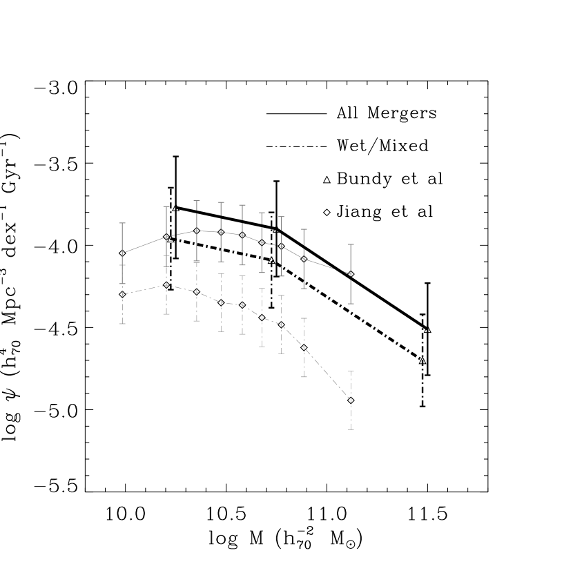
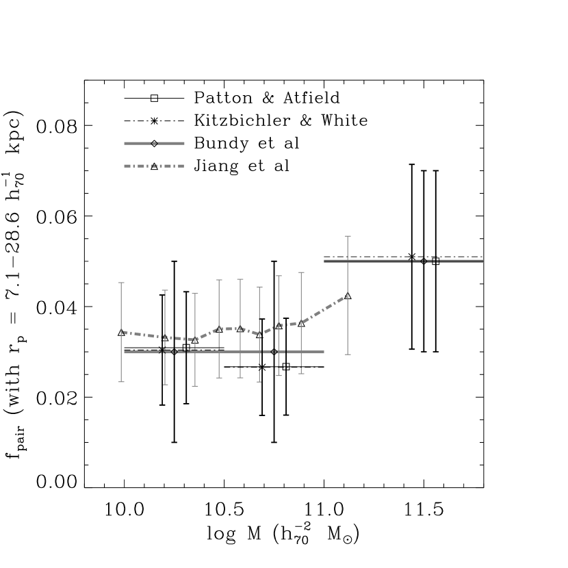
With determined, we compute the volumetric merger rate (the number of mergers per unit time per unit comoving volume) as a function of the stellar mass of the primary or host galaxy. We call this the merger rate mass function (merger rate MF) and denote it using the variable, . Figure 23 shows the comparison of our major merger rate MF at with the major merger rate MF of Bundy et al. (2009) at at mass ratio . We can see that both of Figures 23 and 24 show that our results are consistent with these previous results.
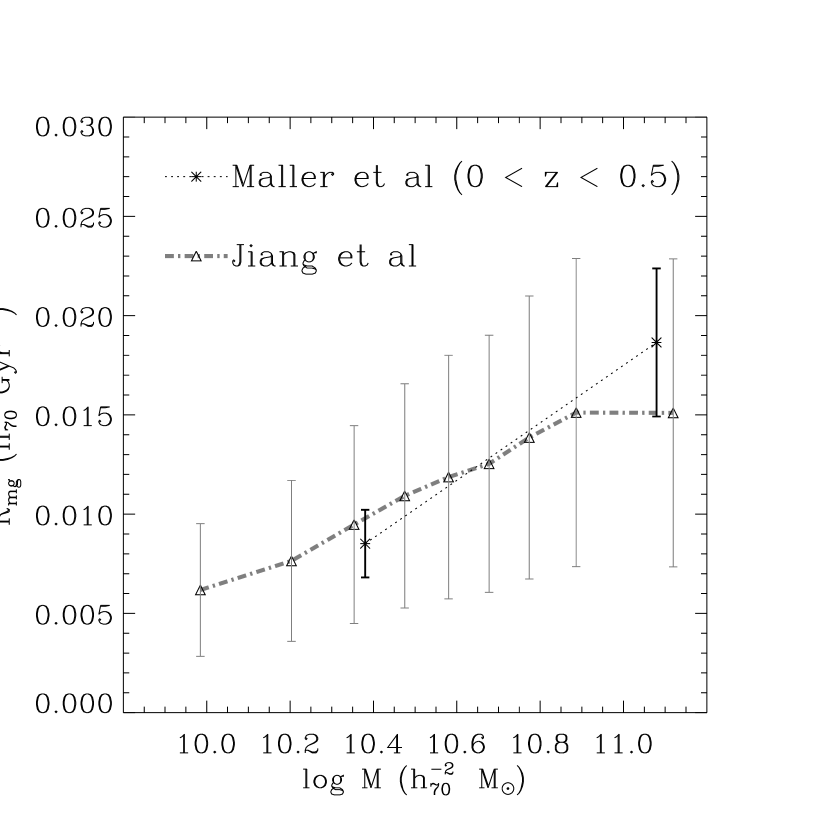
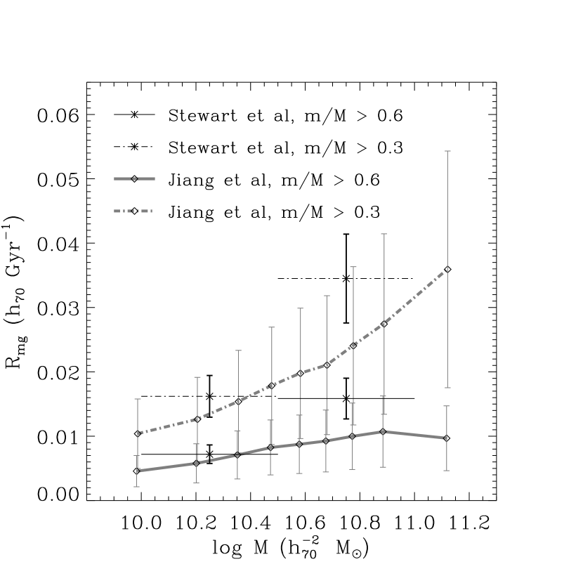
Our results are also consistent with recent merger rates predicted in theories of galaxy formation in a cosmological context (Maller et al., 2006; Stewart et al., 2009). We estimate our merger rate at a certain mass ratio by integrating in equation (29). We compare our with the results of Maller et al. (2006) at mass ratio (Figure 25) and the results of Stewart et al. (2009) at mass ratio and (Figure 26). We can see that both of Figures 25 and 26 show that our results are consistent with these previous results.
Wetzel & Tinker (2012) found that from redshift to now, it is around percent of galaxies similar to our Milky Way that experienced a merger with mass ratio , and around percent that experienced a merger with mass ratio . In our research, the galaxies in blue7 or blue8 subsample are similar to our Milky Way. If we take our results under assumption of at face value and make the strong assumption that the growth happens at a non-evolving rate, from redshift to now (a period of ), we expect the galaxies in blue7 or blue8 subsample to merge by percent with mass ratio , and percent with mass ratio , which is close to the result of Wetzel & Tinker (2012).
5 Discussion
We find that under the assumption of , the total fractional accretion rates onto red main galaxies are from to depending on stellar mass, and those onto blue main galaxies are from to . We find that at fixed stellar mass, the total fractional accretion rates onto red galaxies is greater than that onto blue galaxies. The total fractional accretion rate is a stronger function of primary mass for red galaxies than that for blue galaxies. We also find that more than of the total fractional accretion rates are from major mergers with mass ratio between and , and less than of the total fractional growth rates are from minor mergers with mass ratio between and .
The first limitation of the imaging sample arises from the lack of spectroscopic information on the galaxies from the imaging sample. However, for galaxies from imaging sample with stellar masses , we estimate the real-space number densities from equation (35). So we measured , and separately. But at stellar masses , it is impossible to precisely measure the real-space number densities , so that we cannot disentangle the clustering power from the number density for these small-mass galaxies from the imaging sample, and we only measure the products and but not either , or separately.
The second limitation is removing galaxies from imaging sample with apparent magnitudes because of the limitation of lack of imaging information on the galaxies of SDSS (see Figure 5). This cut of apparent magnitudes will affect the minor mergers with mass ratio between and for the small stellar mass galaxies from spectroscopic samples red14 and blue14 at redshift , and the number densities of the galaxies in these spectroscopic samples decrease sharply at redshift (see Figures 3 and 4), which will sharply reduce the effect of this cut. This cut will cause less than error because the contribution of the minor mergers with mass ratio between and is only . This assumption is good to take, because it will cause far below error. In order to not affect the minor mergers with mass ratio between and at all, we need our imaging sample to be fainter than what we use now.
We can see ‘valleys’ at the third to fifth data points () of the two minor-merger curves ( and ) in each plot of Figures 10 through 13, which seems like a kind of issue due to photometric biases or bad deblending. However we do not think so, because the photometric biases and bad deblending are very small at separations large than (see Table 1) and at ‘valleys’ (the third to fifth data points ), the photometry correction is nearly zero (below ). Also, we do not think that the ‘valleys’ will make our conclusions invalid even if that is an issue in minor merger, because from the above paragraph we know that only less than of the total fractional accretion rates are from minor mergers with mass ratio between and .
If we assume that the growth happens at a non-evolving rate from redshift to now (a period of ), we expect the red galaxies to grow by about to depending on stellar mass under assumption of , and the red galaxies (around red7 and red8) grow by about . The merger rate may have been different in the past, of course, higher or lower (Lin et al., 2008; Chou et al., 2011). If we assume that the growth of massive red galaxies ( galaxies and above) is mainly from galaxy mergers, and also assume that the evolution of the galaxy merger rate per galaxy is proportional to (Lotz et al., 2011) from redshift to now, we expect that the stellar mass density of the red massive galaxies ( galaxies and above) increased about percent under the assumption of , or about percent under the assumption of (see Table 3), which are consistent with recent studies on the high-redshift Universe which find that the red sequence appears to grow in stellar mass over time by a factor of to from redshift to now (Bell et al., 2004; Willmer et al., 2006; Blanton, 2006; Faber et al., 2007; Conselice et al., 2007; Cimatti et al., 2008; van Dokkum et al., 2008; Saracco et al., 2009).
According to Section 4, our results are consistent with the previous clustering results of Zehavi et al. (2010). Our estimated merger rates are consistent with the merger rates estimated by counting of close pairs (Masjedi et al., 2008; Patton & Atfield, 2008; Kitzbichler & White, 2008; Bundy et al., 2009; De Propris et al., 2010; Robaina et al., 2010). Our estimated merger rates are also consistent with the merger rates predicted in theories of galaxy formation in a cosmological context (Maller et al., 2006; Stewart et al., 2009; Wetzel & Tinker, 2012).
However, we found that not all merger studies find such low values when we compared our results with the studies at higher redshift. The morphological derivations of the merger fraction (e.g., De Propris et al. 2007; Conselice et al. 2007; Lotz et al. 2006, 2008; Conselice et al. 2009) tend to find values of at , about times higher than the results of our pair analysis (see Figure 24). The discrepancy can be resolved easily if either (1) morphological signatures of merging last for many dynamical times (e.g., tidal tails) or (2) the very minor mergers () inflate the merger rates (please note that our pair analysis in Figure 24 are only estimated from major mergers at mass ratio ) or (3) morphological tools for finding mergers maybe find some systems which are not involved in mergers or (4) merger rates per galaxy at high redshift may be larger than those at low redshift.
The total fractional accretion rates shown in the solid lines in Figure 19 are upper limits on the true fractional mass growth. There are two reasons: (1) we assume for every pair. However it is not true for close pairs in high velocity dispersion, (2) we assume that the stellar mass growth of the central galaxies from the spectroscopic sample is equal to the stellar mass of the galaxy from the imaging sample, see equation (30). However Lin et al. (2004) found that up to percent of the stars in the galaxies from the imaging sample could be stripped off before the merger with LRGs is complete. So our mass growth rate under the assumption of is an upper limit on the growth by merging.
We find that the accretion onto red and massive blue galaxies is dominated by mergers with red companions, and that onto small-mass blue galaxies, red and blue companions make comparable contributions, this is shown by Table 2 and Figures 17 and 18. So, most of the mass brought into red galaxies by merging is brought by “dry mergers” (Bell et al., 2006b; van Dokkum, 2005; Masjedi et al., 2008).
We find that all the contributions to growth decrease with decreasing stellar mass at the small-mass end for all of 18 spectroscopic subsamples. The contribution to growth decreases with decreasing since . For all 18 subsamples, the curves essentially decrease to zero by for and by for , so calculation of the total amount of mass brought in by merger activities does not require consideration of galaxies from the imaging sample with .
From Figures 10 through 13 and Figure 20, we find a sharp break at and a less-sharp transition at . These two transitions are also found in LRGs by Masjedi et al. (2008), which can be explained in the context of the “halo occupation” picture of galaxy clustering (Peacock & Smith, 2000; Scoccimarro et al., 2001; Berlind & Weinberg, 2002; Cooray & Sheth, 2002; Zheng et al., 2005; Watson et al., 2010, 2012): (1) the mergers at are the one-halo mergers (both of the two merging galaxies are inside one halo); (2) the mergers at are the two-halo mergers (the two merging galaxies are separately inside two nearby halos); (3) the mergers at are the mixed-halo mergers (some of the mergers are the one-halo mergers, the others are the two-halo mergers). So at the mergers transfer from the one-halo mergers to the mixed-halo mergers, and at the mergers transfer from the mixed-halo mergers to the two-halo mergers. These two transitions are clearer in Figure 10 of mergers between two red galaxies than that in the other three figures.
It is a pleasure to thank Douglas Watson, Jeremy Tinker and our anonymous referee for valuable input.
This research made use of public SDSS data. Funding for the SDSS and SDSS-II has been provided by the Alfred P. Sloan Foundation, the Participating Institutions, the National Science Foundation, the U.S. Department of Energy, the National Aeronautics and Space Administration, the Japanese Monbukagakusho, the Max Planck Society, and the Higher Education Funding Council for England. The SDSS Web Site is http://www.sdss.org/.
SDSS is managed by the Astrophysical Research Consortium for the Participating Institutions. The Participating Institutions are the American Museum of Natural History, Astrophysical Institute Potsdam, University of Basel, University of Cambridge, Case Western Reserve University, University of Chicago, Drexel University, Fermilab, the Institute for Advanced Study, the Japan Participation Group, Johns Hopkins University, the Joint Institute for Nuclear Astrophysics, the Kavli Institute for Particle Astrophysics and Cosmology, the Korean Scientist Group, the Chinese Academy of Sciences (LAMOST), Los Alamos National Laboratory, the Max-Planck-Institute for Astronomy (MPIA), the Max-Planck-Institute for Astrophysics (MPA), New Mexico State University, Ohio State University, University of Pittsburgh, University of Portsmouth, Princeton University, the United States Naval Observatory, and the University of Washington.
References
- Abazajian et al. (2003) Abazajian, K. et al. 2003, AJ, 126, 2081
- Abazajian et al. (2004) Abazajian, K. et al. 2004, AJ, 128, 502
- Abraham et al. (1996) Abraham, R. G., Tanvir, N. R., Santiago, B. X., Ellis, R. S., Glazebrook, K., & van den Bergh, S. 1996, MNRAS, 279, L47
- Barnes & Hernquist (1996) Barnes, J. E., & Hernquist, L. 1996, ApJ, 471, 115
- Bell et al. (2004) Bell, E. F., Wolf, C., Meisenheimer, K., Rix, H.-W., Borch, A., Dye, S., Kleinheinrich, M., Wisotzki, L., & McIntosh, D. H. 2004, ApJ, 608, 752
- Bell et al. (2005) Bell, E. F. et al. 2005, ArXiv Astrophysics e-prints
- Bell et al. (2006a) Bell, E. F., Phleps, S., Somerville, R. S., Wolf, C., Borch, A., & Meisenheimer, K. 2006, ApJ, 652, 270
- Bell et al. (2006b) Bell, E. F., et al. 2006, ApJ, 640, 241
- Berlind & Weinberg (2002) Berlind, A. A. & Weinberg, D. H. 2002, ApJ, 575, 587
- Binney & Tremaine (1987) Binney, J., & Tremaine, S. 1987, Princeton, NJ, Princeton University Press, 1987, 747 p.,
- Blanton et al. (2003b) Blanton, M. R. et al. 2003b, ApJ, 594, 186
- Blanton et al. (2005) Blanton, M. R., et al. 2005, AJ, 129, 2562
- Blanton (2006) Blanton, M. R. 2006, ApJ, 648, 268
- Blanton & Roweis (2007) Blanton, M. R., & Roweis, S. 2007, AJ, 133, 734
- Blanton & Moustakas (2009) Blanton, M. R., & Moustakas, J. 2009, ARA&A, 47, 159
- Boylan-Kolchin & Ma (2007) Boylan-Kolchin, M., & Ma, C.-P. 2007, MNRAS, 374, 1227
- Brown et al. (2007) Brown, M. J. I., Dey, A., Jannuzi, B. T., Brand, K., Benson, A. J., Brodwin, M., Croton, D. J., & Eisenhardt, P. R. 2007, ApJ, 654, 858
- Bundy et al. (2006) Bundy, K., et al. 2006, ApJ, 651, 120
- Bundy et al. (2009) Bundy, K., Fukugita, M., Ellis, R. S., Targett, T. A., Belli, S., & Kodama, T. 2009, ApJ, 697, 1369
- Carlberg et al. (1994) Carlberg, R. G., Pritchet, C. J., & Infante, L. 1994, ApJ, 435, 540
- Carlberg et al. (2000) Carlberg, R. G., et al. 2000, ApJ, 532, L1
- Carlberg et al. (2000) Carlberg, R. G., Yee, H. K. C., Morris, S. L., Lin, H., Hall, P. B., Patton, D., Sawicki, M., & Shepherd, C. W. 2000, ApJ, 542, 57
- Chen (2009) Chen, J. 2009, A&A, 494, 867
- Chou et al. (2011) Chou, R. C. Y., Bridge, C. R., & Abraham, R. G. 2011, AJ, 141, 87
- Cimatti et al. (2006) Cimatti, A., Daddi, E., & Renzini, A. 2006, A&A, 453, L29
- Cimatti et al. (2008) Cimatti, A., et al. 2008, A&A, 482, 21
- Conroy et al. (2007) Conroy, C., Ho, S., & White, M. 2007, MNRAS, 379, 1491
- Conselice et al. (2003) Conselice, C. J., Bershady, M. A., Dickinson, M., & Papovich, C. 2003, AJ, 126, 1183
- Conselice et al. (2007) Conselice, C. J. et al. 2007, MNRAS, 381, 962
- Conselice et al. (2009) Conselice, C. J., Yang, C., & Bluck, A. F. L. 2009, MNRAS, 394, 1956
- Cool et al. (2008) Cool, R. J., et al. 2008, ApJ, 682, 919
- Cooray & Sheth (2002) Cooray, A., & Sheth, R. 2002, Phys. Rep., 372, 1
- Courteau et al. (2007) Courteau, S., Dutton, A. A., van den Bosch, F. C., MacArthur, L. A., Dekel, A., McIntosh, D. H., & Dale, D. A. 2007, ApJ, 671, 203
- Daddi et al. (2005) Daddi, E., et al. 2005, ApJ, 626, 680
- Davis & Peebles (1983) Davis, M. & Peebles, P. J. E. 1983, ApJ, 267, 465
- De Propris et al. (2007) De Propris, R., Conselice, C. J., Liske, J., Driver, S. P., Patton, D. R., Graham, A. W., & Allen, P. D. 2007, ApJ, 666, 212
- de Ravel et al. (2009) de Ravel, L., Le Fèvre, O., Tresse, L., et al. 2009, A&A, 498, 379
- De Propris et al. (2010) De Propris, R., et al. 2010, AJ, 139, 794
- Faber et al. (2007) Faber, S. M. et al. 2007, ApJ, 665, 265
- Fukugita et al. (1996) Fukugita, M., Ichikawa, T., Gunn, J. E., Doi, M., Shimasaku, K., & Schneider, D. P. 1996, AJ, 111, 1748
- Gunn et al. (1998) Gunn, J. E., Carr, M. A., Rockosi, C. M., Sekiguchi, M., et al. 1998, AJ, 116, 3040
- Gunn et al. (2006) Gunn, J. E., et al. 2006, AJ, 131, 2332
- Hogg (1999) Hogg, D. W. 1999, arXiv:astro-ph/9905116
- Hogg et al. (2004) Hogg, D. W., et al. 2004, ApJ, 601, L29
- Kartaltepe et al. (2007) Kartaltepe, J. S., et al. 2007, ApJS, 172, 320
- Kitzbichler & White (2008) Kitzbichler, M. G., & White, S. D. M. 2008, MNRAS, 391, 1489
- Li & White (2010) Li, C., & White, S. D. M. 2010, MNRAS, 407, 515
- Lin et al. (2004) Lin, L., et al. 2004, ApJ, 617, L9
- Lin et al. (2008) Lin, L., Patton, D. R., Koo, D. C., et al. 2008, ApJ, 681, 232
- Longhetti et al. (2007) Longhetti, M., et al. 2007, MNRAS, 374, 614
- Lotz et al. (2006) Lotz, J. M., Madau, P., Giavalisco, M., Primack, J., & Ferguson, H. C. 2006, ApJ, 636, 592
- Lotz et al. (2008) Lotz, J. M., et al. 2008, ApJ, 672, 177
- Lotz et al. (2010) Lotz, J. M., Jonsson, P., Cox, T. J., & Primack, J. R. 2010, MNRAS, 404, 590
- Lotz et al. (2011) Lotz, J. M., Jonsson, P., Cox, T. J., et al. 2011, ApJ, 742, 103
- Masjedi et al. (2006) Masjedi, M., et al. 2006, ApJ, 644, 54
- Masjedi et al. (2008) Masjedi, M., Hogg, D. W., & Blanton, M. R. 2008, ApJ, 679, 260
- Maller et al. (2006) Maller, A. H., Katz, N., Kereš, D., Davé, R., & Weinberg, D. H. 2006, ApJ, 647, 763
- Murali et al. (2002) Murali, C., Katz, N., Hernquist, L., Weinberg, D. H., & Davé, R. 2002, ApJ, 571, 1
- Naab & Burkert (2003) Naab, T., & Burkert, A. 2003, ApJ, 597, 893
- Patton et al. (1997) Patton, D. R., Pritchet, C. J., Yee, H. K. C., Ellingson, E., & Carlberg, R. G. 1997, ApJ, 475, 29
- Patton et al. (2000) Patton, D. R., Carlberg, R. G., Marzke, R. O., Pritchet, C. J., da Costa, L. N., & Pellegrini, P. S. 2000, ApJ, 536, 153
- Patton & Atfield (2008) Patton, D. R., & Atfield, J. E. 2008, ApJ, 685, 235
- Patton et al. (2011) Patton, D. R., Ellison, S. L., Simard, L., McConnachie, A. W., & Mendel, J. T. 2011, MNRAS, 412, 591
- Peacock & Smith (2000) Peacock, J. A. & Smith, R. E. 2000, MNRAS, 318, 1144
- Quintero et al. (2004) Quintero, A. D., et al. 2004, ApJ, 602, 190
- Robaina et al. (2010) Robaina, A. R., Bell, E. F., van der Wel, A., Somerville, R. S., Skelton, R. E., McIntosh, D. H., Meisenheimer, K., & Wolf, C. 2010, ApJ, 719, 844
- Scarlata et al. (2007) Scarlata, C., et al. 2007, ApJS, 172, 494
- Scoccimarro et al. (2001) Scoccimarro, R., Sheth, R. K., Hui, L., & Jain, B. 2001, ApJ, 546, 20
- Stewart et al. (2009) Stewart, K. R., Bullock, J. S., Barton, E. J., & Wechsler, R. H. 2009, ApJ, 702, 1005
- Stoughton et al. (2002) Stoughton, C. et al. 2002, AJ, 123, 485
- Strauss et al. (2002) Strauss, M. A., et al. 2002, AJ, 124, 1810
- Strateva et al. (2001) Strateva, I., et al. 2001, AJ, 122, 1861
- Saracco et al. (2009) Saracco, P., Longhetti, M., & Andreon, S. 2009, MNRAS, 392, 718
- Trujillo et al. (2007) Trujillo, I., Conselice, C. J., Bundy, K., Cooper, M. C., Eisenhardt, P., & Ellis, R. S. 2007, MNRAS, 382, 109
- Toft et al. (2007) Toft, S., et al. 2007, ApJ, 671, 285
- van Dokkum et al. (1999) van Dokkum, P. G., Franx, M., Fabricant, D., Kelson, D. D., & Illingworth, G. D. 1999, ApJ, 520, L95
- van Dokkum (2005) van Dokkum, P. G. 2005, AJ, 130, 2647
- van Dokkum et al. (2008) van Dokkum, P. G., et al. 2008, ApJ, 677, L5
- Wake et al. (2006) Wake, D. A. et al. 2006, MNRAS, 372, 537
- Watson et al. (2010) Watson, D. F., Berlind, A. A., McBride, C. K., & Masjedi, M. 2010, ApJ, 709, 115
- Watson et al. (2012) Watson, D. F., Berlind, A. A., McBride, C. K., Hogg, D. W., & Jiang, T. 2012, ApJ, 749, 83
- White et al. (2011) White, M., et al. 2011, ApJ, 728, 126
- Wetzel & Tinker (2012) Wetzel, A., & Tinker, J. 2012, in preparation
- Willmer et al. (2006) Willmer, C. N. A., et al. 2006, ApJ, 647, 853
- York et al. (1999) York, D., et al. 1999, Bulletin of the American Astronomical Society, 31, 1452
- York & SDSS Collaboration (2001) York, D. G., & SDSS Collaboration 2001, Bulletin of the American Astronomical Society, 33, 906
- Zehavi et al. (2005) Zehavi, I., et al. 2005, ApJ, 621, 22
- Zehavi et al. (2010) The SDSS Collaboration: Zehavi et al. 2010, arXiv:1005.2413
- Zepf & Koo (1989) Zepf, S. E. & Koo, D. C. 1989, ApJ, 337, 34
- Zheng et al. (2005) Zheng, Z., et al. 2005, ApJ, 633, 791
- Zhu et al. (2010) Zhu, G., Blanton, M. R., & Moustakas, J. 2010, ApJ, 722, 491
- Zhu et al. (2011) Zhu, G., et al. 2011, ApJ, 726, 110
| Subsample | \ref{1mass}\ref{1mass}footnotemark: | number | \ref{1zmean}\ref{1zmean}footnotemark: | \ref{1zmin}\ref{1zmin}footnotemark: | \ref{1zmax}\ref{1zmax}footnotemark: | or \ref{1velocity}\ref{1velocity}footnotemark: | angular separation\ref{1recover}\ref{1recover}footnotemark: |
|---|---|---|---|---|---|---|---|
| [] | [] | [arcsec] | |||||
| red0 | |||||||
| red1 | and | ||||||
| red2 | and | ||||||
| red3 | and | ||||||
| red4 | and | ||||||
| red5 | and | ||||||
| red6 | and | ||||||
| red7 | and | ||||||
| red8 | and | ||||||
| red9 | and | ||||||
| blue0 | |||||||
| blue1 | and | ||||||
| blue2 | and | ||||||
| blue3 | and | ||||||
| blue4 | and | ||||||
| blue5 | and | ||||||
| blue6 | and | ||||||
| blue7 | and | ||||||
| blue8 | and | ||||||
| blue9 | and |
Note. — Information for the galaxies in the spectroscopic subsamples.
| Subsample | \ref{2df}\ref{2df}footnotemark: | blue fraction \ref{2bluedf}\ref{2bluedf}footnotemark: | \ref{2max}\ref{2max}footnotemark: | blue fraction \ref{2bluemax}\ref{2bluemax}footnotemark: |
|---|---|---|---|---|
| [] | [%] | [] | [%] | |
| red0 | ||||
| red1 | \ref{2error}\ref{2error}footnotemark: | |||
| red2 | ||||
| red3 | ||||
| red4 | ||||
| red5 | ||||
| red6 | ||||
| red7 | ||||
| red8 | ||||
| red9 | ||||
| blue0 | ||||
| blue1 | ||||
| blue2 | ||||
| blue3 | ||||
| blue4 | ||||
| blue5 | ||||
| blue6 | ||||
| blue7 | ||||
| blue8 | ||||
| blue9 |
Note. — Fractional mass growth of Main Galaxy by merging , split by spectroscopic subsample.
| Subsample | \ref{3df}\ref{3df}footnotemark: | \ref{3max}\ref{3max}footnotemark: |
|---|---|---|
| [] | [] | |
| red7 | ||
| red8 | ||
| red9 | ||
| red79 | ||
| red89 | ||
| LRG | ||
| red9 |
Note. — Fractional mass growth measurements for massive red galaxies ( galaxies and above) under assumption of merger rates , split by spectroscopic subsample.


.


