On the stationarity of linearly forced turbulence in finite domains

Abstract

A simple scheme of forcing turbulence away from decay was introduced by Lundgren some time ago, the ‘linear forcing’, which amounts to a force term linear in the velocity field with a constant coefficient. The evolution of linearly forced turbulence towards a stationary final state, as indicated by direct numerical simulations (DNS), is examined from a theoretical point of view based on symmetry arguments. In order to follow closely the DNS the flow is assumed to live in a cubic domain with periodic boundary conditions. The simplicity of the linear forcing scheme allows one to re-write the problem as one of decaying turbulence with a decreasing viscosity. Scaling symmetry considerations suggest that the system evolves to a stationary state, evolution that may be understood as the gradual breaking of a larger approximate symmetry to a smaller exact symmetry. The same arguments show that the finiteness of the domain is intimately related to the evolution of the system to a stationary state at late times, as well as the consistency of this state with a high degree of isotropy imposed by the symmetries of the domain itself. The fluctuations observed in the DNS for all quantities in the stationary state can be associated with deviations from isotropy. Indeed, self-preserving isotropic turbulence models are used to study evolution from a direct dynamical point of view, emphasizing the naturalness of the Taylor microscale as a self-similarity scale in this system. In this context the stationary state emerges as a stable fixed point. Self-preservation seems to be the reason behind a noted similarity of the third order structure function between the linearly forced and freely decaying turbulence, where again the finiteness of the domain plays an significant role.

I Introduction

Maintaining a turbulent flow in a more or less stationary state, for better statistics in experiment or convenience in theoretical considerations, requires forcing the flow, that is feeding it energy which balances dissipation happening at the smallest scales. In numerical simulations of incompressible isotropic turbulent flows one usually solves the Navier-Stokes equations in a cubic box (with periodic boundary conditions). For an account of Direct Numerical Simulation (DNS) methods see moin-mahesh ; for a recent review on the current isotropic turbulence statistics from DNS see DNS-review . In most cases forcing takes the form of a force term in wave number space (spectral space) which vanishes for all but the smaller wave numbers i.e.  one feeds energy at the largest scales of the turbulent flow in the box. The general concept is that the details of the larger scales are model dependent but the details of all other scales, that is those where some universal laws may hold, depend only on the intrinsic dynamics of the Navier-Stokes at least for high Reynolds numbers. Presumably, by forcing turbulence one achieves satisfactory results for given a resolution for higher Reynolds numbers than in the freely decaying turbulence.

There have been developed various kinds of forcing schemes. The simpler ones fiddle in a suitable manner the magnitude of velocity field, or the total energy of the lower wave number modes, imitating an energy input in the larger scales Siggia-forcing ; she-forcing ; chasnov-forcing ; sullivan-forcing . These models can be regarded as essentially deterministic in the sense that that there is no additional randomness introduced in the problem. There are also deterministic models which explicitly introduce a force term in the Navier-Stokes, whose details are either postulated or derived by a postulated auxiliary model kerr-forcing ; siggia2-forcing ; jimenez-forcing ; overholt-forcing . In stochastic forcing models yahkot-forcing ; eswaran-pope ; alvelius the details of the force term are determined by additional random variables following prescribed stochastic processes. Each of those models suffers from one or more from a set of problems such as, excessive fluctuations around stationarity, relatively long relaxation period to stationarity, persistent anisotropy, excessive distortion of large scale motions, introduction of irrelevant features in the description of turbulence. A useful comparative discussion between certain deterministic and stochastic models can be found in TurbulenceIII .

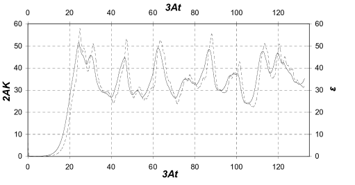
(a)

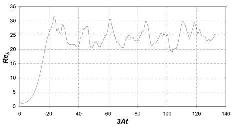
(b)

Figure 1: A typical evolution of the energy production rate (solid line), dissipation rate (dashed line) is shown in the figure (a) and Taylor microscale Reynolds number in figure (b). The parameters chosen are $A=1$, box size $l=2\pi$ and viscosity $\nu=0.1$.

Lundgren proposed in Lund that we may simplify the deterministic models to the bare minimum, in some sense, assuming that the usually velocity dependent force term is merely proportional to the velocity field for all positions $\mathbf{x}$, or all wave numbers $\mathbf{k}$, and all times: $\mathbf{f}=A\mathbf{u}$, where $A$ is plainly a constant. The ‘linear forcing’ scheme was further studied in Rosales and Akylas1 . Its simple force term $A\mathbf{u}$ has the same form in both the spectral and physical space. Thus, unlike other forcing schemes, it may be used equally easy in cases that need to be solved directly in the physical space with boundary conditions different than periodic Rosales . That feature could prove useful. Additionally, although in the linear forcing the injection of energy into the flow is not restricted to the larger scales, this scheme performs decently, and in fact possibly better, in the region between the inertial range and the integral scale than other forcing schemes in Lund . From the theoretical point of view what matters most is that, unlike limited spectral bandwidth forcing schemes, linear forcing does not introduce an additional length scale in the problem at the level of the Navier-Stokes equations (a length scale outside the equations is of course introduced by the boundary conditions).

The performance of the linear forcing scheme with respect to its convergence properties was studied in considerable detail in Rosales and useful remarks have been made in TurbulenceIII . The clear conclusion is that linear forcing results in relatively large fluctuations in the stationary phase. Indeed, a typical evolution of the energy production rate $2AK$ (where $K$ is the total kinetic energy per unit mass), the dissipation rate $\varepsilon$ and the Taylor microscale Reynolds number $\textrm{Re}_{\lambda}$ is shown in fig. 1. [The details of the DNS can be found in Akylas1 ]. From the practical point of view this is a disadvantage as it requires longer simulations in order to obtain good statistics. Also, the stationary state is reached after a relatively long transient period Rosales TurbulenceIII requiring even more computational time. On the other hand, linear forcing leads to quite controllable situations in the stationary state: Given the scales of the problem i.e. the rate $A$, the cubic box size $l$ and the viscosity $\nu$, the facts of the stationary state are predictable. The balance between the energy production and dissipation, $2AK=\varepsilon$, is indeed observed on the (time-)average validating the very concept of a stationary state; the dissipation length $L_{\varepsilon}=(2K)^{\frac{3}{2}}/\varepsilon$ turns out to be equal to the box size $l$ within few percent error in all cases Rosales ; the Reynolds number $\textrm{Re}_{L}=K^{2}/(\varepsilon\nu)$ may be re-written as $\frac{1}{4}AL_{\varepsilon}^{2}/\nu$ at the stationary state, should then be roughly equal to $\frac{1}{4}$ of the natural order of $\textrm{Re}_{L}$ in this problem, $Al^{2}/\nu$, in all cases, as it is indeed observed Akylas1 . For example, the Taylor microscale Reynolds number $\textrm{Re}_{\lambda}=(\frac{20}{3}\textrm{Re}_{L})^{\frac{1}{2}}$ is expected to be roughly equal to 25.7 for the run shown in fig. 1. Indeed the average of the $\textrm{Re}_{\lambda}$ time-series in fig. 1 differs only by few percent from that estimate.

Even if we take stationarity for granted, its characteristics i.e., the relatively large fluctuations and the ‘predictability’ of quantities describing the state of turbulence, certainly call for understanding. On the other hand the very existence of a stationary state in this scheme is a fairly intriguing matter. The long-time effect of the energy production competing with dissipation is not a priori clear. From the dynamical point of view, it is clear that the dissipation term $\nu\nabla^{2}u$ becomes stronger than the force term $Au$ at scales smaller than $(\nu/A)^{\frac{1}{2}}\sim\textrm{Re}_{\lambda}^{-1}l$, but it is not clear whether energy which is produced at all other scales up to $l$ will be dissipated by an adequate rate at those smaller scales.

We will approach the problem as follows. The relative simplicity of linear forcing allows us to study its late-time evolution employing scaling symmetry arguments to an extent enjoyed possibly only in freely decaying turbulence; in fact as we shall show there is a relationship between linearly forced and freely decaying turbulence. A quite parallel discussion between them can be made. The sections II-V will be devoted in presenting these arguments. The predictability, as we called it above, of the stationary state, is enlightened through those symmetry arguments, essentially on the basis that there is no intrinsic large length scale in the dynamical equations apart from that introduced by the boundary conditions i.e. the finite size $l$ of the domain. Then remains the question why the fluctuations observed in the stationary state, as seen e.g. in the fig. 1, are so large. We shall argue, as analytically as we can, that the fluctuations can be associated with the deviations from isotropy accumulated by this forcing at all scales between the scale $(\nu/A)^{\frac{1}{2}}$ and the domain size $l$ (unlike the limited bandwidth forcing schemes which feed anisotropy only at the domain size scale where isotropy is already broken). The method we shall use is to reduce the dynamical problem to a two-equation model. As a cross check of our previous conclusions, the stationary state re-emerges as a stable fixed point of the evolution, a byproduct of which is that fluctuations tend to be suppressed as long as turbulence is isotropic. This part of our discussion is presented mostly in sections VI and VII. It is interesting to note that, from various aspects, linearly forced turbulence seems to be a natural context for the direct application of various ideas that have been developed in the study of freely decaying turbulence, in fact one may dare say, an even more natural context.

In terms of equations, a linearly forced incompressible flow with zero mean flow velocity is described by the Navier-Stokes equation

$$\frac{\partial\mathbf{u}}{\partial t}+(\mathbf{u}\cdot\nabla)\mathbf{u}=-\frac{1}{\rho}\nabla p+\nu\nabla^{2}\mathbf{u}+A\mathbf{u}\,,$$ (1)

where the incompressibility condition reads $\nabla\cdot\mathbf{u}=0$; the velocity field is solenoidal. $A$ is a positive constant with dimensions of inverse time. The term $A\mathbf{u}$ is a curious ‘anti-drag’ force on fluid particles. As already mentioned we impose periodic boundary conditions: $\mathbf{u}(x,y,z)=\mathbf{u}(x,y+l,z)=\mathbf{u}(x,y,z+l)=\mathbf{u}(x+l,y,z)$. That is, the flow evolves within a cubic domain with side equal to $l$ obeying the given conditions on its boundary. (We will often refer to the cubic domain simply as the ‘box’.) As we shall emphasize later on, the term ‘cubic domain’ is slightly misleading due to the periodic boundary conditions: the flow essentially evolves in a boundary-less space of finite size. There are no walls anywhere, this is why we describe the domain as finite instead of bounded. The problem we are interested in to determine the late-time state of the turbulent flow governed by these equations and conditions.

The present work is organized as follows. In sections II and III a reformulation of the problem and an associated scaling symmetry is presented. In section IV the implications of the scaling symmetry and of the symmetries of the domain for the late-time behavior of the ensemble average correlators are discussed. In section V we restrict ourselves to isotropic turbulence, to argue in a more detailed manner for the stationary state as the final phase of the linearly forced turbulence, as described by the exact ensemble average correlators and taking into account the effects of the finiteness of the domain. In section VI the expected behavior of the actual observables in DNS i.e. the box-averaged correlators, is discussed in relation to the properties of the ensemble average correlators established in the previous sections. In section VII we combine the powerful condition of isotropy with the (by now established) existence of fluctuations around stationarity: A complete self-preserving isotropic turbulence model is obtained and applied to study the fate of fluctuations at scales in the flow where isotropy holds. We close with a few additional remarks and discussing certain open issues of the problem in the final section.

II Unforced turbulence with decaying viscosity

We shall proceed as follows. Mathematically, we may re-write the problem as an equation for a new field $\mathbf{u}^{\prime}$ which we require to satisfy

$$\frac{\partial\mathbf{u}^{\prime}}{\partial t^{\prime}}+(\mathbf{u}^{\prime}\cdot\nabla)\mathbf{u}^{\prime}=-\frac{1}{\rho}\nabla p^{\prime}+\nu^{\prime}\nabla^{2}\mathbf{u}^{\prime}\,,$$ (2)

with $\mathbf{u}^{\prime}$ being related to $\mathbf{u}$ by

$$\mathbf{u}^{\prime}=F\,\mathbf{u}\,,$$ (3)

where $F$ is a function of time $F=F(t^{\prime})$ to be determined. $\nabla\cdot\mathbf{u}=0$ implies that $\nabla\cdot\mathbf{u}^{\prime}=0$.

Substituting (3) to (2) we get

$$\frac{1}{F^{2}}\frac{dF}{dt^{\prime}}\mathbf{u}+\frac{1}{F}\frac{\partial\mathbf{u}}{\partial t^{\prime}}+(\mathbf{u}\cdot\nabla)\mathbf{u}=-\frac{1}{F^{2}}\frac{1}{\rho}\nabla p^{\prime}+\frac{1}{F}\nu^{\prime}\nabla^{2}\mathbf{u}\,.$$ (4)

This equation becomes identical to (1) upon setting

$$Fdt^{\prime}=dt\,,\quad\frac{1}{F^{2}}\frac{dF}{dt^{\prime}}=-A\,,\quad\nu^{\prime}=F\nu\,.$$ (5)

The transformation of pressure, $p^{\prime}=F^{2}p$, follows from its Laplace equation constraint and cannot be regarded as an independent condition.

For constant $A$ we have that

$$F=e^{-At}\,,\quad\textrm{and}\quad At^{\prime}+1=e^{At}\,,$$ (6)

where we fix one integration constant by setting $t^{\prime}=0$ corresponding to $t=0$. It is left understood due to the freedom of the second integration consttant that we may shift $t$ arbitrarily.

Viscosity $\nu^{\prime}$ reads

$$\nu^{\prime}=\frac{1}{At^{\prime}+1}\nu\,,$$ (7)

in the unphysical time coordinate $t^{\prime}$. The problem has become unforced turbulence with decaying viscosity. The way it decays, $\propto 1/t^{\prime}$, is crucial in what follows.

Note that everything can be transformed back to the initial variables at all times, except $t=\infty$, or $t^{\prime}=\infty$. This is a singular point of the transformation as $F$ vanishes and the two forms of the problem are not equivalent. That would be a relevant subtlety only if we had to deal with the actual limit $t\to\infty$. We will not need such a limit anywhere in our analysis.

It also worth to note that a transformation $t\to t^{\prime}$ can generate only a term which is linear in $\mathbf{u}$, unless the transformation depends itself on the velocity field. Therefore the possibility of such a generating transformation is intimately related to linear forcing.

III Time-translation invariance and an exact scaling symmetry at late times

Note that equation (1) does not explicitly depend on time, forcing being a function of the velocity field alone. Therefore, depending on boundary conditions, this equation may admit non-trivial solutions which are static or independent of time in a certain sense. As we are interested in fully developed turbulence, the time-dependence in question will apply to statistically defined quantities.

The Navier-Stokes equations we arrived at by transforming to time $t^{\prime}$ in the previous section explicitly reads

$$\frac{\partial\mathbf{u}^{\prime}}{\partial t^{\prime}}+(\mathbf{u}^{\prime}\cdot\nabla)\mathbf{u}^{\prime}=-\frac{1}{\rho}\nabla p^{\prime}+\frac{\nu}{At^{\prime}+1}\nabla^{2}\mathbf{u}^{\prime}\,,$$ (8)

where $\rho$, $\nu$ and $A$ are constants and $\nabla\cdot\mathbf{u}^{\prime}=0$. Apart from the fairly peculiar time-dependence of viscosity, that is, the energy dissipation rate decreases with time, the form of this equation is more familiar than that of equation (1).

Now, the time-translation invariance of equation (1) translates to an exact scaling symmetry of equation (8). Even by inspection one may verify that the transformation

$$t^{\prime}\to e^{a}t^{\prime}\,,\qquad\mathbf{u}^{\prime}\to e^{-a}\mathbf{u}^{\prime}\,,$$ (9)

for any constant $a$ is an exact symmetry of the previous equation (necessarily, $p^{\prime}\to e^{-2a}p^{\prime}$) for times $t^{\prime}\gg A^{-1}$. Then the integration constants in the relation between $t$ and $t^{\prime}$ are irrelevant.

The origin of the late-time scaling symmetry is clear: Shifting $t$ means rescaling $t^{\prime}$, at least for times $t^{\prime}\gg A^{-1}$. Shifting $t$ is a symmetry of equation (1), therefore rescaling $t^{\prime}$ must be a symmetry of equation (8), as it is indeed the case. It is important to remember that the symmetry (9) respects the periodic boundary conditions on the field $\mathbf{u}^{\prime}$, therefore it is an exact symmetry of the problem.

We may now forget equation (1) for a little while and focus on the unforced turbulence described by (8). Its scaling symmetry will allow us to draw certain conclusions about the late time behavior of the system.

IV Scaling symmetries, asymptotic behavior and isotropy

In order to get a first idea why the symmetry can be useful that way, note that the product $t^{\prime}\mathbf{u}^{\prime}$ is invariant under the scaling (9). Consider an arbitrarily chosen moment of time $t_{0}^{\prime}$ and the velocity field $\mathbf{u}_{0}^{\prime}$ at that moment, and another moment $t^{\prime}=e^{a}t_{0}^{\prime}$ when velocity is $\mathbf{u}^{\prime}$. Invariance means: $t^{\prime}\mathbf{u}^{\prime}=t_{0}^{\prime}\mathbf{u}^{\prime}_{0}$. Equivalently we may write

$$\mathbf{u}^{\prime}=\frac{1}{t^{\prime}}\,t_{0}^{\prime}\,\mathbf{u}_{0}^{\prime}\,.$$ (10)

Now in general a symmetry transformation moves us around the space of solutions. That is, all the previous relation means, is that if there is a solution with velocity $\mathbf{u}_{0}^{\prime}$ at time $t_{0}^{\prime}$ then there is another solution with velocity field $\mathbf{u}^{\prime}$ at time $t^{\prime}$. i.e. in general $\mathbf{u}^{\prime}$ and $\mathbf{u}_{0}^{\prime}$ need not necessarily correspond to the same initial conditions.

On the other hand, the symmetry holds for large times $t^{\prime}$ and $t_{0}^{\prime}$. Even if it did not, that would be a convenient choice for the following reason. The initial time $t^{\prime}=0$ is pushed into the remote past, and the behavior (10) might then be an exact asymptotic result for a large class of solutions, meaning irrespectively of their initial conditions. That implies that $t^{\prime}\mathbf{u}^{\prime}=t_{0}^{\prime}\mathbf{u}^{\prime}_{0}$ is an actual constant at each point $\mathbf{r}$ in space depending only on the parameters of the equation and the boundary conditions.

The constant in question is a vector. To be more specific, recalling that $\mathbf{u}^{\prime}$ satisfies $\nabla\cdot\mathbf{u}^{\prime}=0$, we need a solenoidal vector field in steady state which does not depend on initial conditions i.e. it is unique. Such a field must respect the symmetries of the boundary conditions, that is the symmetries of the cube. There is no such thing: solenoidal vector fields have closed integral curves which can always be reversed by reflections. We deduce then that (10), as long as it is non-trivial, will always depend to some extend on $t_{0}^{\prime}$ i.e. on initial conditions. Thus it is not of much use in this form.

Our reasoning can be used more effectively if it is applied in statistically defined quantities, that is, correlators of the velocity field. As mentioned already in the Introduction, from here and up until section VI we shall work with correlators defined as averages over a statistical ensemble. The statistical ensemble averages are independent of the initial conditions by their very definition: they are averages over the space of solutions. Of course in a problem on turbulence they certainly are the quantities of interest. The statistical ensemble averages will be denoted by an overbar.

Then (10) holds trivially for no mean flow: $\overline{\mathbf{u}^{\prime}}=0$. Next one considers general correlators of the velocity field, $\overline{u^{\prime}_{i_{1}}(\mathbf{r}_{1},t^{\prime}_{1})u^{\prime}_{i_{2}}(\mathbf{r}_{2},t^{\prime}_{2})\cdots}$, and their derivatives. Consider local correlators i.e. all times and positions coincide. These are tensor fields $T^{\prime}_{j_{1}j_{2}\cdots}(\mathbf{r},t^{\prime})$. Let such a tensor field with $n$ velocity field insertions in the correlation. Then the symmetry (9) tells us, similarly to (10), that

$$T^{\prime}_{j_{1}j_{2}\cdots}=\frac{1}{t^{\prime n}}\,t^{\prime n}_{0}\,T^{\prime}_{0\,j_{1}j_{2}\cdots}\,.$$ (11)

Now $t^{\prime n}_{0}\,T^{\prime}_{0\,j_{1}j_{2}\cdots}(\mathbf{r},t_{0}^{\prime})$ must be a constant at each point $\mathbf{r}$ in space. If not, then this quantity does depend on $t_{0}^{\prime}$ i.e. on the initial conditions. That means: this quantity is not well defined as a ensemble average i.e. mathematically does not exist and it must be defined in an approximate manner which does not possess the expected properties, or only approximately. The reason why this may happen is that the system has not reached a stage where ensemble averages are meaningful, a priori some kind of equilibrium is required.

Now, same as with $t_{0}^{\prime}\mathbf{u}^{\prime}_{0}$, most of these constant tensor fields must be zero by being inconsistent with the symmetries of the cube (especially reflections) and the incompressibility condition. Certainly everything with at least one solenoidal index must vanish. This leaves us with the scalars, tensors manufactured out of them and Kronecker delta, and correlators such as $\overline{\partial_{i}u_{k}\partial_{j}u_{k}}$ with no free solenoidal index.

In order to see how these statements are realized by an example, consider the correlator $t^{\prime 2}_{0}\,\overline{u^{\prime}_{0i}u^{\prime}_{0k}}$, which is constant in time. Being constant in time means that it must respect the symmetries of the cubic domain: it must not change under reflections of the domain around planes of symmetry and rotations around axis of symmetry. One should recall that our correlators are ensemble averages over the whole of phase space, thus symmetries cannot take us to an other constant late-time solution: there is no other solution, or we have convergence problems in the very definition of our averages. It is then easy to see that $t^{\prime 2}_{0}\,\overline{u^{\prime}_{0i}u^{\prime}_{0k}}$ must be equal to $\delta_{ik}\,t^{\prime 2}_{0}\,\overline{u^{\prime}_{0i}u^{\prime}_{0i}}(\textrm{no sum})=\frac{1}{3}\delta_{ik}\,t^{\prime 2}_{0}\,\overline{u^{\prime}_{0j}u^{\prime}_{0j}}$, i.e. essentially a scalar. Moreover, by the incompressibility condition $\nabla\cdot\mathbf{u}^{\prime}=0$ we see that the scalar itself must be constant in space.

One should note that the situation resembles very much that of isotropic i.e. also homogeneous turbulence. There is anisotropy allowed by the problem but it is much less than what would call anisotropy in general. Thus we will proceed by assuming isotropy and analyze what that implies; then, as isotropy cannot hold at scales comparable to the cubic box size $l$, the effects of the boundary eventually play a key role. This is done in the next section. We close this section by defining a few important scalars for the description of turbulence, their symmetry and transformation properties and their expected late time behavior according to our arguments.

The r.m.s. value $q$ of the velocity and the dissipation rate $\varepsilon$ are defined by $q^{2}=\overline{\mathbf{u}\cdot\mathbf{u}}$ and $\varepsilon=\nu\,\overline{\partial_{j}u_{i}\partial_{j}u_{i}}$. Also by $K=\frac{1}{2}q^{2}$ we shall denote the total kinetic energy per unit mass. Similar expressions hold for the primed quantities.

Under the symmetry (9) the quantities $K^{\prime}$ and $\varepsilon^{\prime}$ transforms as

$$K^{\prime}\to e^{-2a}K^{\prime}\,,\qquad\varepsilon^{\prime}\to e^{-3a}\varepsilon^{\prime}\,,$$ (12)

where one should bear in mind that $\varepsilon^{\prime}$ involves $\nu^{\prime}$ defined in (7). Following again the reasoning given in the previous paragraphs we conclude that for large times $t^{\prime}$ the kinetic energy and dissipation rate should obey

$$K^{\prime}=\frac{\textrm{constant}}{t^{\prime 2}}\,,\qquad\varepsilon^{\prime}=\frac{\textrm{constant}}{t^{\prime 3}}\,.$$ (13)

In order to see what this result means back in the variables of the system (1), we use (3) and (7) to obtain the transformations of $K$ and $\varepsilon$:

$$K^{\prime}=(At^{\prime}+1)^{-2}K\,,\qquad\varepsilon^{\prime}=(At^{\prime}+1)^{-3}\varepsilon\,.$$ (14)

The result is then that the kinetic energy and dissipation rate in the linearly forced turbulence should at late times become

$$K=\textrm{constant}\,,\qquad\varepsilon=\textrm{constant}\,.$$ (15)

Presumably, the dissipation length scale $L_{\varepsilon}$ and the Reynolds number $\textrm{Re}_{L}$ defined by

$$L_{\varepsilon}=\frac{q^{3}}{\varepsilon}\,,\qquad\textrm{Re}_{L}=\frac{K^{2}}{\varepsilon\nu}\,,$$ (16)

and transforming by

$${\textrm{Re}^{\prime}}_{\!\!L}=\textrm{Re}_{L}\,,\qquad{L^{\prime}}_{\!\!\varepsilon}=L_{\varepsilon}\,,$$ (17)

should also reach constant values. That is, turbulence should get to what we have already called as the stationary state or phase.

***

The arguments given above can be rephrased in the actual time $t$ and the variables of equation (1) as follows. We have already mentioned that shifting time $t$ is a symmetry of equation (1). That is, if $\mathbf{u}(t)$ is a solution of this equation then so is $\mathbf{u}(t+\Delta t)$ for an arbitrary interval $\Delta t$. These two solutions do not coincide because they correspond to the different initial conditions. On the other hand, we may say that for a certain class of initial conditions, that difference should become irrelevant at late times i.e. the two solutions, or at least certain quantities calculated out of them, will coincide. But this is the same as stating the obvious fact that static or stationary solutions of (1) exist, without explaining whether such stationary states are indeed the ending point of solutions for an reasonably large class of initial conditions. In this light our arguments as given so far seem rather trivial.

Our arguments are essentially about symmetries. The most convenient context to discuss them, and possibly the only context, is that of isotropic turbulence. We shall argue that the evolution of the system to the stationary phase, can be thought of as the gradual breaking of a larger approximate symmetry to the smaller exact symmetry (9), which is solely consistent with the stationary state. That will be realized in certain convenient cases where one may convince oneself that one ‘watches’ the system evolving as claimed. By the very form of (8) one may guess that standard knowledge from the freely decaying turbulent flows could prove useful to us.

We start by reviewing certain useful facts about the freely decaying isotropic turbulence.

V Homogeneous and isotropic turbulence

V.1 Important quantities and formulas

Consider homogeneous and isotropic turbulence. The one-direction r.m.s. value of the velocity, $q_{1}$, does not depend on the direction, i.e.  $q^{2}=3q_{1}^{2}$. The two-point correlation function of the velocity is reduced to a scalar $f(r)$ which depends only the distance $r$ between the two points: $\overline{u_{l}(0)u_{l}(\mathbf{r})}=q_{1}^{2}\,f(r)$. The entire information of the two-point correlation is contained in components $u_{l}$ longitudinal in the direction of separation. Also the two-point triple correlation of the velocity can only have longitudinal components and it is expressed in terms of a scalar $h(r)$ by $\overline{u_{l}(0)u_{l}(0)u_{l}(\mathbf{r})}=q_{1}^{3}\,h(r)$. A priori all quantities depend on time, for that reason time-dependence is left understood.

Equation (1) with $A=0$ is the unforced Navier-Stokes equation describing turbulence in the freely decaying state. The ‘Karman-Howarth equation’ LandauFluidMechanics Frisch derived from it under the conditions of homogeneity and isotropy reads

$$\frac{\partial}{\partial t}(q_{1}^{2}f)=\frac{1}{r^{4}}\frac{\partial}{\partial r}\Big{\{}r^{4}\Big{(}q_{1}^{3}\,h+2\nu\,q_{1}^{2}\,\frac{\partial f}{\partial r}\Big{)}\Big{\}}\,.$$ (18)

In freely decaying turbulence the rate at which energy $K$ is decreasing equals the dissipation rate $\varepsilon$, expressing the balance of total energy in that problem.

$$\dot{K}=-\varepsilon\,.$$ (19)

Presumably, this also holds if the viscosity $\nu$ depends explicitly on time. This fact will be useful below.

The integral scale, $L\equiv\int_{0}^{\infty}\!fdr$, is of the order of magnitude of the dissipation length $L_{\varepsilon}$. The Taylor micro-scale $\lambda_{g}$ is defined by a differential relation involving $f$:

$$\lambda_{g}^{2}\left.\frac{\partial^{2}f}{\partial r^{2}}\right|_{r=0}\!\!\!=-1\,,\quad\textrm{i.e.\ }\quad\lambda_{g}=\sqrt{\frac{10\nu K}{\varepsilon}}\,.$$ (20)

For completeness, and as we shall briefly need it later on, we write down the energy balance equation for the spectral densities of $K$ and $\varepsilon$. It is a Fourier transform of the Karman-Howarth equation (18), see e.g. Frisch .

$$\partial_{t}E(k)=-\partial_{k}T(k)-2\nu k^{2}E(k)\,.$$ (21)

The ‘spectrum’ $E(k)$ suitably integrates to give the kinetic energy and dissipation rate, $K=\int_{0}^{\infty}E(k)dk$ and $\varepsilon=2\nu\int_{0}^{\infty}k^{2}E(k)dk$. $T(k)$ is the spectral energy flux and vanishes for vanishing and infinite wave numbers. Clearly (19) follows by integrating (21) over all $k$, though the derivation of energy balance equations will be discussed in more detail section VI.

V.2 Scaling symmetries and power laws

The scaling arguments given in this section are borrowed from Oberlack1 . The method is an application of the reasoning presented in section IV.

Consider the Karman-Howarth equation (18). Now perform the two-parameter scaling transformation

$$t\to e^{a}t\,,$$

$$r\to e^{b}r\,,$$

$$q\to e^{b-a}q\,,$$ (22)

$$f\to f\,,$$

$$h\to h\,,$$

for arbitrary constants $a$ and $b$. Changing $a$ for fixed $t$ amounts to time evolution from the initial moment $t$. Similarly changing $b$ for fixed $r$ amounts to looking at larger distances. Under (V.2) equation (18) becomes

$$\frac{\partial}{\partial t}(q_{1}^{2}f)=\frac{1}{r^{4}}\frac{\partial}{\partial r}\Big{\{}r^{4}\Big{(}q_{1}^{3}\,h+e^{a-2b}\,2\nu\,q_{1}^{2}\,\frac{\partial f}{\partial r}\Big{)}\Big{\}}\,.$$ (23)

Consider high Reynolds numbers. Then the viscosity term can be dropped. We see then that the transformation (V.2) is an approximate symmetry of (18) for high Reynolds numbers; it can be regarded as a symmetry of the system for infinite Reynolds numbers.

Consider then quantities of interest such as the kinetic energy $K$, or the integral scale $L$ (equivalently, the dissipation length $L_{\varepsilon}$). They transforms same as $q^{2}$ and $r$ respectively.

The one-parameter subgroup of the transformation (V.2) such that

$$\gamma=\frac{b}{a}\,,$$ (24)

is an arbitrary but fixed number, given explicitly by

$$t\to e^{a}t\,,$$

$$r\to e^{\gamma a}r\,,$$

$$q\to e^{\gamma a-a}q\,,$$ (25)

$$f\to f\,,$$

$$h\to h\,,$$

for arbitrary $a$, leaves the quantities

$$t^{-\gamma}L\,,\qquad t^{2-2\gamma}K\$$ (26)

invariant.

Note that this way, we think of the two-parameter group (V.2) as one-parameter ($\gamma$) family of one-parameter subgroups (V.2). Presumably, equation (23) becomes identical to (18) iff $a-2b=0$ that is $a-2\gamma a=0$. This means that the subgroup $\gamma=\frac{1}{2}$ is an exact symmetry of the freely decaying turbulence. In other words, the larger symmetry (V.2) for infinite Reynolds number breaks down to its subgroup $\gamma=\frac{1}{2}$ for finite Reynolds numbers.

Each symmetry (V.2) is essentially time-evolution. Following the arguments of section IV we conclude that at adequately late times

$$L=\textrm{constant}\,\,t^{\gamma}\,,\qquad K=\textrm{constant}\,\,t^{2\gamma-2}\,.$$ (27)

Thus we have obtained certain power laws for the late behavior of the length scale and kinetic energy in freely decaying turbulence. The law for the dissipation rate $\varepsilon$ follows immediately by (19),

$$\varepsilon=\textrm{constant}\,t^{2\gamma-3}\,.$$ (28)

Then, by (16) the law for dissipation length $L_{\varepsilon}$ turns out consistent with that of $L$, as course it should. The law for $\textrm{Re}_{L}$ also follows from (16):

$$\textrm{Re}_{L}=\textrm{constant}\,t^{2\gamma-1}\,.$$ (29)

Summarizing, each value of $\gamma$ defines a subgroup of the full symmetry group (V.2) for high Reynolds. Given a $\gamma$ the time-dependence of various quantities takes the form of specific power laws. A priori not fixed without additional conditions, the exponent $\gamma$ may be given an additional physical interpretation. Assume that for low wave-numbers $k$ the spectrum $E(k)$ is of the form

$$E(k)=Ck^{\sigma}+o(k^{\sigma})\,,$$ (30)

for some constants $C$ and $\sigma$. Given the dimension of $E(k)$ and $k$ and the constancy of $C$, this relation is invariant under (V.2) iff

$$\gamma=\frac{2}{\sigma+3}\,.$$ (31)

That is, the subgroup (V.2) is fixed by the small wave-number behavior of the spectrum of the specific class of flows. It may be argued, see e.g. Ref. Lesieur , that $C$ is actually constant as long as $1\leq\sigma<4$; also the case $\sigma=4$ holds marginally. That is, in those cases $C$ is fixed by the initial conditions.

Decay exponents are usually expressed in terms of $n\equiv 2-2\gamma$, which is the kinetic energy decay exponent, $K\sim t^{-n}$. About the value of $n$ there are well known suggestions. They depend upon the identification of $C$ with quantities which are conserved under certain conditions. Kolmogorov K41-decay and Batchelor Batchelor48 , based on the conservation of the Loitsyanky integral Loitsianski , derived $\gamma=\frac{2}{7}$ i.e. $n=\frac{10}{7}$. Saffman Saffman1 set forth the hypothesis that the vorticity and not the velocity correlator is an analytic function in spectral space, by which rediscovered the $\sigma=2$ spectrum and Birkhoff’s integral Birkhoff-Turbulence and derived $\gamma=\frac{2}{5}$ i.e. $n=\frac{5}{6}$. Experimentally Comte-Bellot-Corssin Warhaft-Lumley both values of the decay exponent $n$ are acceptable. The value $n=1$ has also been suggested by other theoretical considerations, for high but finite Reynolds numbers Speziale and as the limiting value of the decay exponent for infinitely high Reynolds numbers george-92:1492 ; Barrenblatt-book ; lin ; this solution first appeared in dryden .

The $n=1$ decay solution for finite Reynolds numbers of Ref. Speziale can be obtained by recalling an observation given above, that for finite Reynolds numbers the symmetry (V.2), essentially associated with infinite Reynolds numbers, breaks down to its $\gamma=\frac{1}{2}$ subgroup at finite Reynolds numbers. That means $n=1$. Presumably, by (29), the Reynolds number is constant for this solution.

The $n=1$ decay law may also be obtained in another way, which gives the chance to make an additional comment on the analysis presented in this section. The Taylor microscale $\lambda_{g}$ transforms as a length, same as $r$, according to the equation on the left in (20). That means that $\lambda_{g}=\textrm{constant}\,t^{\gamma}$. On the other hand the equation on the right in (20) and the laws (27) and (28) imply $\lambda_{g}=\textrm{constant}\,t^{\frac{1}{2}}$. The reason why there is no discrepancy is because regarding $L$ as finite and Reynolds number virtually infinite, for the symmetry (V.2) to hold, means that $\lambda_{g}$ is virtually zero. Put differently, if we want to think of the previous analysis as applying also to high but finite Reynolds numbers, then we must restrict ourselves to scales much larger than Taylor microscale. It is then no accident that the power laws (27) can also be produced by models deriving from self-similarity of turbulence with respect to the integral scale $L$, as we shall discuss in section VII. On the other hand if we want finite Reynolds and to take into account scales of $O(\lambda_{g})$ or less, then it must be $\gamma=\frac{1}{2}$ i.e. $n=1$.

Being such a direct implication of the arguments in this section, one may wonder why the $n=1$ decay solution is not observed experimentally even for the highest Reynolds numbers (equivalently, as $\gamma=\frac{1}{2}$ means $\sigma=1$, a small wave-number spectrum $E(k)\propto k$ has not been verified). The arguments possibly fail on the very part where one expects independence from the initial conditions. That expectation might be in a better shape the higher, still finite, the Reynolds number is. This is why in the best case the $n=1$ solution can possibly be regarded as describing well decaying turbulence for very high Reynolds numbers.

In the next two subsections we come to the problem of interest. The discussion parallels in some sense our previous remarks: Going from the infinitely high to any lower Reynolds number the larger symmetry (V.2) breaks in this case down to its exact subgroup $\gamma=0$ associated with the linearly forced turbulence, the exact symmetry (9) we started our discussion with. But, unlike the freely decaying case, in our problem a large length scale and a Reynolds number scale are necessarily present, eventually forcing the system towards the $\gamma=0$ evolution. That amounts to reaching the stationary state.

V.3 Linearly forced isotropic turbulence

Consider linearly forced turbulence in the description given by equation (8), which let us state again:

$$\frac{\partial\mathbf{u}^{\prime}}{\partial t^{\prime}}+(\mathbf{u}^{\prime}\cdot\nabla)\mathbf{u}^{\prime}=-\frac{1}{\rho}\nabla p^{\prime}+\frac{\nu}{At^{\prime}+1}\nabla^{2}\mathbf{u}^{\prime}\,.$$

The analogue of the transformed Karman-Howarth equation (23) for late times $t^{\prime}\gg A^{-1}$ reads now

$$\frac{\partial}{\partial t^{\prime}}(q^{\prime 2}_{1}f^{\prime})=\frac{1}{r^{4}}\frac{\partial}{\partial r}\Big{\{}r^{4}\Big{(}q^{\prime 3}_{1}h^{\prime}+e^{-2\gamma a}\frac{\nu}{At^{\prime}}2q^{\prime 2}_{1}\,\frac{\partial f^{\prime}}{\partial r}\Big{)}\Big{\}}\,.$$

We find of course again that the subgroup $\gamma=0$ of the group (V.2) i.e. the group (9), is an exact late-time symmetry of the linearly forced turbulence. For very high Reynolds numbers the larger group (V.2) is a good approximate symmetry of the system. The evolution laws for the dimensionful quantities are necessarily similar to those of the freely decaying case,

$$L^{\prime}=\textrm{constant}\,\,t^{\prime\gamma}\,,$$ (32)

$$K^{\prime}=\textrm{constant}\,\,t^{\prime 2\gamma-2}\,,$$

$$\varepsilon^{\prime}=\textrm{constant}\,t^{\prime 2\gamma-3}\,.$$

while the dimensionless Reynolds number has a different power law due to the time-varying $\nu^{\prime}$:

$$\textrm{Re}^{\prime}_{L}=\textrm{constant}\,t^{\prime 2\gamma}\,.$$ (33)

Consider a flow that starts off with velocities of order $u_{0}$ and a box of size $l$ such that $u_{0}\gg Al$. Equivalently the turn-over time is much smaller than forcing time scale $A^{-1}$, that is, $l/u_{0}\ll A^{-1}$.

Given $A$, $l$ and $\nu$ there is a naturally defined Reynolds number in the problem:

$$\textrm{Re}_{A}=\frac{Al^{2}}{\nu}\,.$$ (34)

That is, the condition $l/u_{0}\ll A^{-1}$ can be rephrased as that the flow starts off with a very high Reynolds number, $\textrm{Re}_{L}\gg\textrm{Re}_{A}$.

Consider then times $t^{\prime}$ such that $l/u_{0}\ll t^{\prime}\ll A^{-1}$. Looking at the previous equation we understand that for those times the turbulent flow is merely freely decaying with constant viscosity $\nu$. If all previous inequalities hold strongly enough, then there will be time for the flow to evolve adequately towards its developed stage. That means that the quantities describing turbulence will evolve according to the power laws (32) and (33).

When $t^{\prime}$ becomes of order of $A^{-1}$ ‘linear forcing’ kicks in. Now one should recall that Reynolds number is always decreasing, therefore some time before or after that moment it will drop enough so that the viscosity term cannot be neglected. That means that from that moment on the group (V.2) is not much of a symmetry anymore: the only symmetry remaining is its subgroup (9) corresponding to $\gamma=0$, which is exact and therefore holds at all times. Viscosity now decreases with time therefore energy will be dissipated with an ever decreasing rate. We may then picture, very roughly, the flow evolving by going through stages of smaller exponents $\gamma$, following simple of less simple laws parameterized by it, eventually reaching the specific value for which a subgroup (V.2) is an exact symmetry of the system: $\gamma=0$.

Let us recapitulate. There is a symmetry existing in the system for high Reynolds numbers. A priori allows for arbitrary values of the parameter $\gamma$. This symmetry breaks down to its subgroup $\gamma=0$ when Reynolds drops enough. This is an exact symmetry of the system, therefore holds always. The final state must be the one respecting that exact symmetry. The power laws (32) and (33) imply that $L^{\prime}$ and $\textrm{Re}_{L}^{\prime}$ are constant, $\varepsilon^{\prime}=\textrm{constant}\,t^{\prime-3}$ and $K^{\prime}=\textrm{constant}\,t^{\prime-2}$. The transformations (14) and (17) back to the original variables of equation (1) show that everything, that is $K$, $\varepsilon$, $L_{\varepsilon}$ and $\textrm{Re}_{L}$, is constant. We have reached the stationary state. $K^{\prime}$ and $\varepsilon^{\prime}$, which are time-dependent in the description (8) of the problem, are related by the equation (19) written down for the primed quantities:

$$\frac{dK^{\prime}}{dt^{\prime}}=-\varepsilon^{\prime}\,.$$ (35)

The (32) and (33) power laws for $\gamma=0$ and the transformations (14) translate that relation to

$$2AK=\varepsilon\,.$$ (36)

That is, at the stationary state energy production balances exactly dissipation.

If initially Reynolds number is not very high, there will be a strong mixing of the phases of freely decaying and ‘linear forced’ turbulence. The transition between them is then too complicated to describe. Though one cannot argue against the possibility the system having an entirely different behavior, it seems reasonable that the same mechanisms which lead the system to the power laws consistent with $\gamma=0$ will do the same thing, in far more complicated way.

V.4 Effects of the finite domain

A very amusing thing we observe is that, by (31), the value $\gamma=0$ corresponds to $\sigma=\infty$. This indicates that the power law behavior of the spectrum $E(k)$ for small wave-numbers degenerates, and should be replaced by some other, much faster decreasing law, perhaps some kind of exponential.

There is a good reason why we expect that. The system (1), or (8), is solved in a domain of some finite size $l$. An infinite size $l$ is meaningless: In the absence of another large length scale, this means that the total energy production rate in the domain depends on it and diverges, $2AK\rho l^{3}\to\infty$. Also large $l$ essentially means a large $Al$ compared with any specific initial condition $u_{0}$: an infinitely large $l$ is equivalent to initial conditions $u_{0}$ infinitely close to zero. Now finite size means that there are no wave-numbers $k$ between $O(l^{-1})$ and zero, therefore any continuous approximation of the spectrum $E(k)$ must fall very rapidly for $kl$ smaller than $O(1)$.

There is a major implication following the presence of a finite size domain. Its fixed size $l$ breaks the symmetry (V.2), as the presence of a fixed length says that it must be $b=0$. That is, the domain size breaks the larger symmetry (V.2) down to its subgroup $\gamma=0$, the exact symmetry.

We may now think of the evolution of the flow from another point of view, that of the integral scale. As long as the integral scale $L^{\prime}$ is small compared to $l$ the group (V.2) is a fairly good approximate symmetry. Then $L^{\prime}$ increases with time as $\sim t^{\prime\gamma}$. As $L^{\prime}$ grows larger, (V.2) is a less and less good approximate symmetry. As before, we may then roughly picture the flow as going through stages of smaller $\gamma$ reaching the stage with $\gamma=0$ which is consistent with the exact symmetry. This means that $L^{\prime}$ will become constant. The natural order for that constant $L^{\prime}$ (as well as $L$, recalling that $L=L^{\prime}$ by the transformation (17)) is the domain size $l$. As mentioned in the Introduction, DNS have shown that specifically $L_{\varepsilon}=l$ within a few percent error Rosales .

We may note that for high Reynolds numbers the viscosity term can be anyway neglected. Therefore the (32) and (33) power laws for $\gamma=0$ and the arguments given above, make sense for very high Reynolds numbers for freely decaying turbulent flows in a finite domain. The difference in the ‘linearly forced’ case (8) is that those power laws are associated with an exact symmetry of the equations and of course hold also for lower Reynolds numbers. In contrast, as we have seen in section V.2, the exact symmetry in the freely decaying turbulence requires $\gamma=\frac{1}{2}$. Linearly forced turbulence behaves in a simpler way than the freely decaying, in this sense.

One should note that by the time linear forcing kicks in, the time-dependence of viscosity $\nu^{\prime}$ changes the form of the Reynolds number power law. During times that linear forcing is already at work but the Reynolds number is still very high compared to $\textrm{Re}_{A}$ and decreasing, the Reynolds number is given by the power law (33) and decreases due to a decreasing $\gamma$ as we argued in the previous section. That is, when $\gamma$ eventually vanishes the peculiar ‘decaying’ turbulent flow (8) reaches a peculiar kind of stationarity: its Reynolds number becomes constant i.e. turbulence as such is not decaying at all. This reflects of course the association of this state to an scaling exact symmetry of the full viscous equations. Recalling transformation (17), $\textrm{Re}_{L}^{\prime}=\textrm{Re}_{L}$, this is also the Reynolds number of the linearly forced turbulence described in the variables of (1).

That final value of the Reynolds number can be easily estimated by the existence of a natural scale $\textrm{Re}_{A}$, defined in (34). At the stationary state energy production balances dissipation, $2AK=\varepsilon$, which implies that $\textrm{Re}_{L}=AL_{\varepsilon}^{2}/(4\nu)$ i.e. $\textrm{Re}_{A}$ indeed sets the scale for the Reynolds number at the stationary state. In fact, as mentioned in the Introduction, DNS show that $\textrm{Re}_{L}=\frac{1}{4}\textrm{Re}_{A}$ within a few percent error Akylas1 .

We conclude that the finiteness of the domain emerges as a crucial factor in understanding the flow evolving to a stationary state. Now the domain, we often referred to as the ‘box’, should be understood more carefully in terms of periodicity. This is what we discuss next.

VI The state of isotropy

In the previous section we restricted ourselves to flows obeying the conditions of homogeneity and isotropy. Let us review what that involves. Contract (1) with $\mathbf{u}$ and average. After a little re-arranging we have

$$\frac{\partial K}{\partial t}=-\varepsilon+2AK++\nu\nabla^{2}K-\nabla\cdot\mathbf{J}\,,$$ (37)

$$\textrm{J}_{i}\equiv\overline{\Big{(}\frac{u^{2}}{2}+\frac{p}{\rho}\Big{)}u_{i}}\,.$$

Homogeneity alone makes all locally defined correlators, such as $K$ or $J_{i}$, independent of the position in space. That is, the last two terms in the last equation vanish. Of course everywhere isotropy means homogeneity, so if the flow is assumed isotropic those two terms go again away. We are then left with

$$\dot{K}=-\varepsilon+2AK\,.$$ (38)

In a stationary state we get $\varepsilon=2AK$, whose form we already anticipated on dimensional grounds deriving the final value (34) of the Reynolds number in terms of the box size $l$.

We should now recall that the box is a cubic domain together with periodic boundary conditions we impose on all fields. The periodic boundary conditions can be given some enlightening interpretations. One way to think of them is that we solve the Navier-Stokes in an infinite medium imposing periodicity $l$ on the field $\mathbf{u}(x,y,z)$ in all three directions $x$, $y$ and $z$. That in turn means that homogeneity is not a priori broken: a box such that $\mathbf{u}(x,y,z)$ satisfies periodic boundary conditions can be drawn anywhere in the infinite medium. By the periodicity we apparently restrict ourselves to special kinds of flow such that there is an upper bound to the size of eddies or any spatially periodic structure in it.

Another way to think of the periodic boundary conditions is to interpret them as mere single-valued-ness of the fields while identifying the points of the boundary of the cube where the fields are supposed to be equal. This may be pictured if we go one dimension down. If we take a square and identify the opposite sides we get a topological torus. A torus is a perfectly homogeneous space without boundary which is non-trivial globally and it is not isotropic. Imposing periodic boundary conditions on the cube means we essentially solve Navier-Stokes equations on the three-dimensional analogue of such a space, the three-torus.

An implication of periodicity and its peculiar nature is that an analogue of the equation (38) holds without assuming point-wise homogeneity of the flow. Let us denote by $\langle X\rangle$ the spatial average over the volume of the box of a quantity with an ensemble average $X$. Averaging that way we get an equation similar to (37) for box-averages

$$\frac{d\langle K\rangle}{dt}= -\langle\varepsilon\rangle+2A\langle K\rangle+$$

$$+\frac{1}{V_{\textrm{box}}}\int_{\textrm{bdy}}\{\nu\nabla K-\mathbf{J}\}\cdot d\mathbf{a}\,.$$ (39)

The last term is a surface integral over the boundary surface of the box. This integral is a sum of

$$\int_{x=l}(\nu\partial_{x}K-J_{x})dydz-\int_{x=0}(\nu\partial_{x}K-J_{x})dydz$$ (40)

plus two more analogous pairs of terms for the other two directions. As all fields are manufactured out of correlations of the field $\mathbf{u}$ which satisfies periodicity $\mathbf{u}(x,y,z)=\mathbf{u}(x+l,y,z)$, and the same for the other two directions, any pair of terms such as (40) vanishes exactly and identically. In other words even if point-wise homogeneity is not assumed, periodicity implies that

$$\frac{d\langle K\rangle}{dt}=-\langle\varepsilon\rangle+2A\langle K\rangle$$ (41)

must hold exactly.

Alternatively, the vanishing of the boundary term in (VI) follows automatically under the interpretation that we solve our problem on a three-torus: there simply is no boundary, $x=0$ and $x=l$ describe the same surface somewhere on the three-torus. Whatever the interpretation of the boundary conditions, one ends up with (41) without assuming homogeneity of the flow.

This is a good thing to know. The box-averaged correlators $\langle X\rangle$ are the actual observables in the DNS. Now, what is their relation to the ensemble averages $X$? Assuming that $X$ are meaningful and under an ergodic hypothesis, $X$ are represented by averaging $\langle X\rangle$ over suitable and adequately large intervals of time. That first of all means that although the motion of $\langle X\rangle$ is not the same as that of $X$ it should nonetheless be bounded and appear as fluctuating around hypothetical stationary values. This is what it is observed, fig. 1. Those values should of course be the values of the correlators $X$.

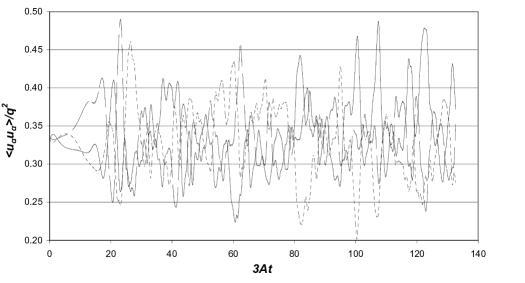
Figure 2: Time evolution of the diagonal components of the normalized Reynolds stresses, $\langle u_{\alpha}u_{\alpha}\rangle/q^{2}$(no sum), from the same run producing the time-series in fig. 1.

Contemplating the far more complicated motion of the correlators $\langle X\rangle$ compared to that of $X$, one quickly realizes that both kinds of correlators obey the same basic dynamical equations. Thus their difference lies somewhere else. The simplicity of the motion of $X$ follows from their independence from the initial conditions of the flow and the symmetries of the dynamical equations and of the domain. Correlators $\langle X\rangle$ are not a priori independent of the initial conditions of the flow and none of the arguments of section IV applies to them. Therefore there are many more and more complicated solutions $\langle X\rangle$ than $X$.

In particular, in section IV it was emphasized that the symmetries of the cube, combined with the symmetry (9), force a fair amount of isotropy on the solutions $X$. That will hold only on the average for the correlators $\langle X\rangle$. This is the actual result of numerical simulations, fig. 2.

We consider the fluctuations of measures of isotropy important for the following reason. The ‘fair amount of isotropy’ exhibited by $X$ is not so harmless itself: Reasonably, any anisotropy is inherited by the correlators $\langle X\rangle$ and it is enhanced in their description of turbulence. The origin of any enhancement of anisotropy is that in linear forcing there is no intrinsic large scale at which we feed the flow energy in some isotropic manner; the large scales are set by the domain itself and the scales comparable to its size are necessarily not isotropic. Subsequently, anisotropy is produced and maintained at those and smaller scales through forcing and cascade. Although the motion of the correlators $X$ suggests that the system cannot be kicked off balance, the produced anisotropy will cause relatively large fluctuations of all quantities $\langle X\rangle$ describing turbulence.

In the next section we will try to lend some quantitative support to this intuitive picture. If deviations from isotropy are related to the fluctuations of all quantities then any fluctuations should vanish in a perfectly isotropic setting. That may give us a sense of what happens when those fluctuations are continually generated. As we shall see the analysis is interesting in its own right as it reveals rather important dynamical properties of linearly forced turbulence.

VII Self-preserving turbulence and stability of stationarity

Studying the fluctuations around the stationary state is equivalent to studying the stability of that state as a fixed point of solutions, in the statistical sense. In fact, this is an alternative way to look at the main problem we have been concerned with, the stationary state as an attractor of solutions. Of course, such an analysis is a very difficult thing to do unless we resort to some suitable simplification.

According to the plan set at the end of the previous section, we shall assume that the flow is isotropic. Therefore all correlators involved, which can be thought of either as ensemble correlators $X$ or box-averages $\langle X\rangle$, are assumed to have the properties required by that condition. We may then investigate the fate of any deviations away from the stationary state if the flow evolves remaining isotropic.

The evolution laws derived in the previous sections can be alternatively derived in isotropic turbulence from models relating the kinetic energy $K$ and dissipation rate $\varepsilon$. These models can be deduced on dimensional grounds, or more systematically by self-similarity arguments, which are fairly equivalent to the scaling arguments given here. The latter date back to the work of von Karman and Howarth KH and Batchelor Batchelor48 , see also Townsend Batchelor-Book . One looks for self-similar solutions of the equations w.r.t. a single length scale $L(t)$, ‘self-preserving’ turbulent flows. Assuming that the larger scales of the flow are evolving in such a self-preserving manner, one chooses $L(t)$ to be the integral scale and one obtains a closed system of equations for the variables $K$ and $\varepsilon$. That simple model can also be regarded as describing self-preserving turbulence of all scales but for infinitely high Reynolds numbers, essentially for inviscid flow.

One can straightforwardly apply the same arguments in the linearly forced turbulence. The spectral energy balance equation (21) becomes

$$\partial_{t}E(k)=-\partial_{k}T(k)-2\nu k^{2}E(k)+2AE(k)\,.$$ (42)

The origin of the additional term should be clear. Then the self-preserving development of the larger scales of the flow implies, via standard steps which can be found e.g. in Townsend Batchelor-Book , the model equation

$$\frac{d\varepsilon}{dt}=-C^{A}_{\varepsilon}\frac{\varepsilon^{2}}{K}+c_{1}A\varepsilon\,,$$ (43)

where $c_{1}=3$ and $C^{A}_{\varepsilon}$ is a dimensionless constant. Apart from the value of $c_{1}$, this equation could also have been guessed on dimensional grounds upon requiring its r.h.s. to be built out of $\varepsilon$ and $K$ and $A$ and be linear in $A$.

Integrating (42) over all wave numbers we obtain again the exact equation (38), which we write down again for convenience,

$$\frac{dK}{dt}=-\varepsilon+2AK\,.$$ (44)

The system of equations (44) and (43) is consistent with a static solution only for $2C^{A}_{\varepsilon}=c_{1}$. The special case $C^{A}_{\varepsilon}=c_{1}/2=3/2$, predicted by large scale self-preservation, implies that $L_{\varepsilon}=\textrm{constant}$ at all times the model holds. This is consistent with the general idea about it. The large scale self-preservation model equation (43) and the value $C_{\varepsilon}^{A}=3/2$ will emerge again from a different perspective in section VIII. The model can be easily solved exactly and indeed predicts that the flow approaches stationarity exponentially fast for all $C^{A}_{\varepsilon}>1$ (the case $C^{A}_{\varepsilon}=1$ is trivially consistent with stationarity).

A more elaborate analysis of the evolution of isotropic turbulence has been presented in the past in the Refs. George-1987 George-1989 Speziale george-92:1492 . In those works the self-similarity hypothesis is applied at the viscous equations of the flow i.e. self-preservation is required to be true for all scales of turbulence for finite Reynolds. In the terminology of Ref. Speziale , self-preservation is complete. An implication of this requirement is that the self-similarity scale is the Taylor microscale $\lambda_{g}$.

From the point of view of the linearly forced turbulence all that sound very relevant and interesting for the following reasons. First, the linearly forced turbulence comes to the intelligible part of its course when its Reynolds number approaches the value (34) which need not be very high at all; second, energy is generated uniformly at all points in the domain and it feels that all scales play a role in approaching or maintaining stationarity; and third, in this problem there is a natural scale for the Taylor length $\lambda_{g}$. It is the scale at which energy production balances dissipation in spectral space, as can be seen by equation (42):

$$\lambda_{A}=\sqrt{\frac{\nu}{A}}\,.$$ (45)

This is designated as a Taylor microscale because the stationary state value of the Taylor microscale, $\lambda_{gs}$, is of that order:

$$\lambda_{gs}=\sqrt{5}\lambda_{A}\,.$$ (46)

This follows from the definition (20) of $\lambda_{g}$ and the stationary state total balance of energy production balances dissipation, $2AK=\varepsilon$. For these reasons the Taylor microscale may be regarded as playing a particularly significant role in the dynamical aspects of linear forcing, perhaps quite more significant than in the freely decaying case. [On the other hand, as everything turns out approaching constancy, eventually the integral scale might be used as a self-similarity scale, a choice associated with the model (43), providing a more crude and late-time description of the evolution of the system.] In any case this choice does provide a closed two-equation model with some interesting properties.

We may then proceed as follows. There is another exact equation which we may use along with (44). One way to derive it is to start from the Karman-Howarth equation for linearly forced isotropic turbulence

$$\frac{\partial}{\partial t}(q_{1}^{2}f)=\frac{1}{r^{4}}\frac{\partial}{\partial r}\Big{\{}r^{4}\Big{(}q_{1}^{3}\,h+2\nu\,q_{1}^{2}\,\frac{\partial f}{\partial r}\Big{)}\Big{\}}+2A\,q_{1}^{2}f\,,$$ (47)

applying the definitions (49) below. (The spectral energy balance equation (42) is a Fourier transform of (18).) Alternatively, and more instructively, we can do everything from scratch by differentiating $\varepsilon$ w.r.t. to time using its very definition as an ensemble or box-average correlator. Then, employing the Navier-Stokes equation (1) and applying the condition of isotropy on any arising correlator one arrives at

$$\frac{d\varepsilon}{dt}=\frac{7|S|}{3\sqrt{15\nu}}\,\varepsilon^{3/2}-\frac{7G}{15}\frac{\varepsilon^{2}}{K}+2A\varepsilon\,,$$ (48)

where $S$ (the velocity gradient distribution skewness) and $G$ are defined by

$$S=\lambda_{g}^{3}\left.\frac{\partial^{3}h}{\partial r^{3}}\right|_{r=0}\,,\qquad G=\lambda_{g}^{4}\left.\frac{\partial^{4}f}{\partial r^{4}}\right|_{r=0}\,,$$ (49)

where $f$ and $h$ are the two-point double and triple point correlations of the velocity defined in section V.1. Equation (48) can also be derived by multiplying (42) by $2\nu k^{2}$ and use formulas equivalent to (49) and (20) in wave number space.

The system of equations (44) and (48) is not closed, the dependence of $S$ and $G$ on $K$ and $\varepsilon$ is unknown. Assume now that at some moment $t_{0}$ the flow becomes self-similar with a (time-dependent) similarity scale $\lambda_{0}$. That means $f$ and $g$ are functions of the dimensionless coordinate $r/\lambda_{0}$ alone, modulo a possible dependence on the initial conditions at $t_{0}$. Now (20) tells us that $\lambda_{0}/\lambda_{g}$ must be a constant, depending only on the initial conditions at $t_{0}$. Thus the similarity scale is indeed the Taylor microscale. Then by (49) we have that $S$ and $G$ are constant and equal to the values they have at $t_{0}$: $S=S_{0}$ and $G=G_{0}$. Now the system (44) and (48) is closed and we may study it.

Let us denote the stationary state values of the dissipation rate and kinetic energy by $\varepsilon_{s}$ and $K_{s}$. Of course they are related by $\varepsilon_{s}=2AK_{s}$. We would like to study the stability properties of $\varepsilon=\varepsilon_{s}$ and $K=K_{s}$ as a complete self-preserving solution of the system of equations (44) and (48).

It will be convenient to define the quantity

$$g\equiv\frac{7G_{0}}{15}\,.$$ (50)

First of all, equation (48) implies that

$$\varepsilon_{s}^{1/2}=2A\frac{3\sqrt{15\nu}}{7|S_{0}|}\,(g-1)\,,$$ (51)

which implies that

$$g>1\,.$$

It is useful to relate the value of $g$ to the Taylor-scale Reynolds number $\textrm{Re}_{\lambda}=(\frac{20}{3}\textrm{Re}_{L})^{\frac{1}{2}}$. By (16) we find that its stationary value $\textrm{Re}_{\lambda s}$ reads

$$\textrm{Re}_{\lambda s}=\frac{30}{7|S_{0}|}\,(g-1)\,.$$ (52)

Define now small fluctuations $\xi$ and $\zeta$ of $\varepsilon$ and $K$ around their stationary values:

$$\varepsilon=\varepsilon_{s}\,(1+\xi)\,,\quad K=K_{s}\,(1+\zeta)\,.$$ (53)

Inserting these expressions into (44) and (48) and keeping only linear terms we obtain the following system of equations:

$$\frac{d\xi}{dt}=-A(1+g)\,\xi+2Ag\,\zeta\,,$$ (54)

$$\frac{d\zeta}{dt}=-2A\,\xi+2A\,\zeta\,.$$

Its eigenvalues $\Gamma$ read

$$\Gamma=\frac{1}{2}A\left(-(g-1)\pm\sqrt{(g-1)(g-9)}\right)\,.$$ (55)

By $g>1$ we see that the real part of both eigenvalues is always negative. Fluctuations around the stationary state die out exponentially fast. That is, modulo finite domain effects, the stationary state is stable as a complete self-preserving isotropic solution. We may also view this result as providing further evidence that the stationary state is the natural final state of the linearly forced turbulence. [Presumably, one may observe that exponentially fast approach to the stationary state is also the prediction of the simpler model (43).]

The previous analysis can be alternatively understood as follows. In order to derive the previous results we have assumed perfect isotropy. A reasonable assumption about the deviations from isotropy is that they originate from scales of order $l$. That means, according to our conclusions in the previous section, that the same can be said about the fluctuations around the stationary state. That is, one may attribute the generation of fluctuations to the interaction of the larger eddies with the periodicity i.e. the restriction to their size. Then, through both forcing and cascade, fluctuations are generated at all scales from $l$ down to a certain scale where isotropy becomes a good approximation. There things are different. We may define correlators as spatial averages $\langle X\rangle_{V}$ over volumes $V$ smaller than that maximum isotropic scale i.e. within these volumes turbulence is isotropic (meaning homogeneity as well) to a good approximation. Then $K$ and $\varepsilon$ understood as spatial averages $\langle X\rangle_{V}$ obey similar equations to those studied above. The entire previous analysis goes through. That finally means that at adequately small scales the fluctuations are strongly suppressed, but at all higher scales are maintained through forcing and cascade. The maximum isotropic scale should be (very) roughly related to the characteristic Taylor microscale of linear forcing $\lambda_{A}=(\nu/A)^{\frac{1}{2}}$, as below that scale dissipation becomes stronger to energy production.

We may investigate the linear system (54) a bit further. Though this system meant to serve us mainly for qualitative considerations, regarding the stability of the constant solution $K=K_{s}$ and $\varepsilon=\varepsilon_{s}$, there are some amusing remarks to be made about it solutions on the quantitative side. In the range $1<g<9$ the eigenvalues $\Gamma$ are complex numbers. If we take for definiteness $|S_{0}|=0.5$, that means that when $\textrm{Re}_{\lambda}<69$ the fluctuations are damped oscillations. [Presumably, this emergence of oscillations is a qualitative difference between the complete self-preservation model and the simpler model (43).] Inserting the solutions $\zeta=\zeta_{0}e^{\Gamma t}$and $\xi=\xi_{0}e^{\Gamma t}$, for positive frequency into any of the equations (54) we obtain the phase difference and the relative amplitude of $\varepsilon$ and $K$:

$$\xi_{0}=\sqrt{g}\,e^{-i\phi}\,\zeta_{0}\,,$$ (56)

where $\phi$ is given by

$$\tan\phi=\frac{\sqrt{(g-1)(9-g)}}{g+3}\,.$$ (57)

As expected the dissipation $\varepsilon$ evolves with a phase delay w.r.t. the kinetic energy $K$ and the energy production $2AK$. This corresponds to a time-delay $\phi/|\textrm{Im}\Gamma|$. The period of these damped oscillations is of course $2\pi/|\textrm{Im}\Gamma|$.

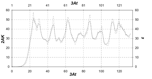
Figure 3: The time evolution of the dissipation rate $\varepsilon$ which is shown in fig. 1, is shifted in this figure by one unit of dimensionless time $3At$.

In fig. 1 we plotted the energy production $2AK$ and dissipation rate $\varepsilon$ against time in units of $(3A)^{-1}$. Now let us shift the evolution of dissipation by one unit of time to off-set its delay. The result is given in the fig. 3. One observes that after that shift the complicated oscillations appear in phase to a considerable degree of accuracy. Curiously, the time-delay $\phi/|\textrm{Im}\Gamma|$ in units of $(3A)^{-1}$ decreases from $1.5$ to $0.5$ in the range $1<g<9$. Also the period $2\pi/|\textrm{Im}\Gamma|$ is roughly an order of magnitude higher than $(3A)^{-1}$ for most values of $g$, which as a number is not in disagreement with the picture in fig. 3. Given that these numbers derive from a model which does not interact with the source of the fluctuations, it seems interesting that the oscillations it implies may encapsulate certain features of the actual fluctuation. There certainly is no identification between the actual fluctuations and those oscillations. For example, when $g\sim 9$ that is $\textrm{Re}_{\lambda s}\sim 70$ the damped oscillations are replaced by a purely decaying exponential, a qualitative change in the behavior which cannot be traced in the DNS results of the Refs. Rosales Akylas1 TurbulenceIII .

(a)

(b)

(c)

Figure 4: Time evolution of the kinetic energy (solid line) and dissipation (dashed line) normalized by their stationary state values from numerical solutions of the system (58). Figure (a): initial conditions $\hat{K}(0)=1.3$ and $\hat{\varepsilon}(0)=1.2$ for $g=2.2$ that is $\textrm{Re}_{\lambda s}\sim 10$. Figure (b): $\hat{K}(0)=0.01$ and $\hat{\varepsilon}(0)=0.01$ for the same value of $g$. Figure (c): $\hat{K}(0)=0.01$ and $\hat{\varepsilon}(0)=0.01$ for $g=9.9$ that is $\textrm{Re}_{\lambda s}\sim 85$.

The previous remarks derive from the quantitative characteristics of small fluctuations, and we may have over-extended the applicability of the related formulas. Arbitrary fluctuations are described by the solutions of the full non-linear model (44) and (48). This needs to be solved numerically. In terms of the dimensionless (hatted) kinetic energy, dissipation rate and time, defined respectively by $K=K_{s}\,\hat{K}$, $\varepsilon=\varepsilon_{s}\,\hat{\varepsilon}$ and $\hat{t}=2At$, the non-linear model reads

$$\frac{d\hat{K}}{d\hat{t}}=-\hat{\varepsilon}+\hat{K}\,,$$ (58)

$$\frac{d\hat{\varepsilon}}{d\hat{t}}=(g-1)\,\hat{\varepsilon}^{3/2}-g\frac{\hat{\varepsilon}^{2}}{\hat{K}}+\hat{\varepsilon}\,.$$

The parameter $g$ is related to $\textrm{Re}_{\lambda s}$ by (52) and we again take for definiteness $|S_{0}|=0.5$.

The system (58) is solved using the software Mathematica. We consider a few specific cases. First, the difference of the initial conditions from the stationary state values is such that to imitate the size of the observed fluctuations. This is shown in fig. 4a. Second, the kinetic energy $\hat{K}$ and dissipation rate $\hat{\varepsilon}$ start off from very close to zero, shown in fig. 4b. For those two cases we have chosen an adequately small Reynolds number so that oscillations to be visible. Finally we consider the effect of higher Reynolds numbers. An evolution of $\hat{K}$ and $\hat{\varepsilon}$ for $\textrm{Re}_{\lambda s}\sim 85$ is shown in fig. 4c.

The result is that the picture is not qualitatively different than the one obtained from the small fluctuations. In the figs. 4a and 4b, the time-delay of the dissipation relatively to the kinetic energy and the period of the damped appear essentially as predicted previously, and the oscillations of the dissipation are consistently larger as implied by equation (56). On the other hand fig. 4b shows a particular behavior of the non-linear solutions: if the initial condition is far away from the stationary state values the system undergoes large fluctuations before settling to those values. The fig. 4c shows that increasing the Reynolds number any wiggling of the curves due to oscillatory behavior diminishes to extinction, which is again what we expected.

VIII discussion

Direct numerical simulations of turbulence forced by the linear forcing scheme exhibit a not entirely expected stationary late-time state. The stationary phase is essentially quasi-stationary: all quantities have relatively large fluctuations, though their time-average can be predicted fairly well. In the present work we have attempted to understand how these phenomena are rooted in the properties of the system. This was done by using the symmetries of the dynamical equations of the problem, as well as the symmetries associated with the boundary conditions i.e. the size and the symmetries of the cubic domain; also, using special dynamical properties of the system derived under usually employed conditions such as exact isotropy or self-similarity. In this problem there are few and specific scales: the domain size $l$, the constant rate $A$ and the viscosity $\nu$. Out of them derive a Taylor microscale $\lambda_{A}$ and a Reynolds number $\textrm{Re}_{A}$. These quantities control the major (intelligible) features of linearly force turbulence evolution.

The importance of the finiteness of the domain and its effects cannot be over-emphasized in the linearly forced turbulence. In a limited bandwidth forcing scheme, deterministic or stochastic, the inverse wave numbers at which one forces the flow imitate, very roughly, the scale of a physical stirring of an incompressible fluid existing in slightly larger ’box’. In linear forcing there is no such intrinsic scale. This simplifies things in some sense because there is no interaction between the forcing and domain size scales. On the other hand it is left entirely to the domain to set the large scales, becoming an essential part of the forcing itself. Also the large scale is introduced geometrically as a matter of size and not dynamically as in the bandwidth schemes, and there is no actual control over the extent forcing is consistent with isotropy. Turbulence is expected to behave quite differently under linear forcing than under a bandwidth scheme. There some additional interesting properties of linear forcing we have not yet commented on. These properties can be associated with the effects of the finite domain size, and also show an at least formal affinity of the linear forcing to freely decaying turbulence, than to the bandwidth forcing schemes.

Denote by $\Delta u_{l}$ the longitudinal velocity difference. The second and third order structure functions are related to the correlation functions $f$ and $h$, introduced in section V, by $\overline{(\Delta u_{l})^{2}}=2q_{1}^{2}(1-f)$ and $\overline{(\Delta u_{l})^{3}}=6q_{1}^{3}h$. For adequately high Reynolds numbers there is a range of distances (the inertial range) where $\overline{(\Delta u_{l})^{2}}=C_{2}(\varepsilon r)^{2/3}$, where $C_{2}$ a constant. Consider first decaying turbulence. It evolves according to the power laws (27), the integral scale is proportional to $t^{\gamma}$. The law for $\varepsilon$ can be deduced. It is then straightforward to show that they satisfy the $K-\varepsilon$ model equation (43) for

$$C_{\varepsilon}=\frac{3-2\gamma}{2-2\gamma}\,,$$ (59)

and of course $A=0$. Using the Karman-Howarth equation (18) it then straightforward to show Lindborg lund-2 that for very high but finite Reynolds numbers, and within the inertial range (more specifically as long as $r/\lambda_{g}$ is a number of $O(1)$), the two-thirds law of the second order structure function implies specific finite Reynolds number corrections to the four-fifths law of the third order structure function, of $O(\textrm{Re}_{\lambda}^{-2/3}$). The result is Lindborg lund-2

$$\qquad\overline{(\Delta u_{l})^{3}}=-\frac{4}{5}\varepsilon r\times$$ (60)

$$\left(\!1-\frac{5\times 15^{\frac{2}{3}}}{17}C_{\varepsilon}C_{2}\textrm{Re}_{\lambda}^{-\frac{2}{3}}\Big{(}\!{\frac{r}{\lambda_{g}}}\!\Big{)}^{\frac{2}{3}}-\Big{(}\!\frac{25}{3}\!\Big{)}^{\frac{1}{3}}C_{2}\textrm{Re}_{\lambda}^{-\frac{2}{3}}\Big{(}\!\frac{r}{\lambda_{g}}\!\!\Big{)}^{-\frac{4}{3}}\right).$$

Consider the same question in the linearly forced turbulence. One may follow the same steps, starting from the Karman-Howarth equation with linear forcing, equation (47). One finds a result entirely similar to (60) upon replacing

$$C_{\varepsilon}\to-\frac{K}{\varepsilon^{2}}\frac{d\varepsilon}{dt}+\frac{3AK}{\varepsilon}\,.$$ (61)

Observe now that if we think of the r.h.s. of this substitution as a constant, then we re-discover the model equation (43); the constant is what we denoted there by $C_{\varepsilon}^{A}$. Equation (43) is derived assuming self-similarity (self-preservation) of the larger scales of turbulence with respect to the integral scale $L$ for high Reynolds numbers, in both the linearly forced ($A\neq 0$) and freely decaying case ($A=0$). In all, by self-preservation we obtain a similar result of the form (60) in both kinds of turbulence, differing only in the value of the constants $C^{A}_{\varepsilon}$ and $C_{\varepsilon}$. On the linearly forced side, self-preservation requires $C_{\varepsilon}^{A}=3/2$ and equation (43) and (44) require that $L=\textrm{constant}$. At first sight there is no such restriction on the freely decaying side. In all, there appears to be a correspondence between linearly forced and freely decaying turbulence, though this correspondence appears inexact.

Now if we require $C_{\varepsilon}^{A}=C_{\varepsilon}$ then by (59) we have that $\gamma=0$. In other words, if the decaying turbulence evolves according to $L\sim\textrm{constant}$ (and $K\sim t^{-2}$) then its structure function expression (60) is exactly similar to that of the linearly forced turbulence. That is, the correspondence between the two flows can be exact.

The $K\sim t^{-2}$ evolution is too fast compared to the usually observed decay laws, discussed in section V.2. Such power laws can be reproduced if choose the constant $C_{\varepsilon}$ to be different than 3/2, a fact regarded as an imperfection of the correspondence in the Ref. Lund , where it was first pointed out. On the other hand the origin and the nature of the correspondence seem to have been overlooked in Lund .

The key role is played again by the finiteness of the domain. As emphasized in section V.4 a container is a necessary thing when turbulence is linearly forced. Lacking an intrinsic length scale, linear forcing essentially requires a large scale to be provided by the boundary conditions. It is therefore not much of a surprise that similarities between linearly forced and freely decaying turbulence are more detailed when the decaying side evolves in a way consistent with the existence of a container: For adequately high Reynolds numbers that means $L\sim\textrm{constant}$ (and the rest of the (27)-(29) power laws for $\gamma=0$). Then the mathematics of self-similarity of turbulence with respect to the scale $L$ imply exactly the same formula (60) for both kinds of turbulence.

The next obvious question is, what kind of modifications does linear forcing need in order to reproduce aspects of a generic decaying turbulence, associated with (59) and an evolution law $L\sim t^{\gamma}$? Two immediate guesses are to consider a time-dependent rate $A=A(t)$ or, to consider a time-dependent box whose size $l$ evolves according to $l\sim t^{\gamma}$. The analysis of such possibilities is left for future work.

References

- (1) P. Moin and K. Mahesh, “Direct numerical simulations: A tool in turbulence research,” Annu. Rev. Fluid Mech. 30 (1990) 539–578.
- (2) T. Ishihara, T. Gotoh, and Y. Kaneda, “Study of high-Reynolds number isotropic turbulence by direct numerical simulation,” Annu. Rev. Fluid Mech. 41 (2009) 165–180.
- (3) E. D. Siggia and G. S. Patterson, “Intermittency Effects in a Numerical Simulation of Stationary Three-Dimensional Turbulence,” J. Fluid Mech. 86 (1978) 567.
- (4) Z.-S. She, E. Jackson, and S. A. Orszag, “Statistical aspects of vortex dynamics in turbulence,” in New Perspective in Turbulence, ed. L. Sirovich, Springer, Berlin, 1991.
- (5) J. R. Chasnov, “Simulation of the Kolmogorov inertial subrange using an improved subgrid model,” Phys. Fluids A 3 (1991) 188.
- (6) N. Sullivan, S. Mahalingam, and R. Kerr, “Deterministic forcing of homogeneous, isotropic turbulence,” Phys. Fluids 6 (1994) 1612.
- (7) R. M. Kerr, Theoretical investigation of a passive scalar such as temperature in isotropic turbulence. PhD thesis, Cornell University, 1981.
- (8) E. D. Siggia, “Numerical study of small-scale intemittency in three-dimensional turbulence,” J. Fluid Mech. 107 (1981) 375–406.
- (9) J. Jimenez, A. A. Wray, P. G. Saffman, and R. S. Rogallo, “The structure of intense vorticity in isotropic turbulence,” J. Fluid Mech. 255 (1993) 65–90.
- (10) M. R. Overholt and S. B. Pope, “A deterministic forcing scheme for direct numerical simulations of turbulence,” Comput. Fluids 27 (1998) 11–28.
- (11) V. Yahkot, S. A. Orszag, and R. Panda, “Computational test of the renormalization group of turbulence,” Journal of Scientific Computing 3(2) (1988) 139–147.
- (12) V. Eswaran and S. B. Pope, “An examination of forcing in direct numerical simulations of turbulence,” Comput. Fluids 16 (1988) 257–278.
- (13) K. Alvelius, “Random forcing of three-dimensional homogeneous turbulence,” Phys. Fluids 11 (1999) 1880–1889.
- (14) Z. Zeren and B. Bedat, “Spectral and physical forcing of turbulence,” in Springer Proceedings in Physics 131, Progress in Turbulence III, Proceedings of the iTi Conference in Turbulence 2008, pp. 9–12.
- (15) T. S. Lundgern, “Linearly forced isotropic turbulence,” in Annual Research Briefs of Center for Turbulence Research, Stanford, 2003, pp. 461–472.
- (16) C. Rosales and C. Meneveau, “Linear forcing in numerical simulations of isotropic turbulence: Physical space implementations and convergence properties,” Phys. Fluids 17 (2005) 095106.
- (17) E. Akylas, S. C. Kassinos, D. Rousson, and X. Xu, “Accelerating Stationarity in Linearly Forced Isotropic Turbulence,” in Proc. of the 6th International Symposium on Turbulence and Shear Flow Phenomena, South Corea, June 2009, pp. 22–24.
- (18) L. D. Landau and E. M. Lifshitz, Fluid Mechanics. Pergamon Press, 1987.
- (19) U. Frisch, Turbulence The Legacy of A. N. Kolmogorov. Cambridge University Press, 1995.
- (20) M. Oberlack, “On the decay exponent of isotropic turbulence,” Proc. Appl. Math. Mech. 1 (2002) 294–297.
- (21) M. Lesieur, Turbulence in Fluids. Kluwer Academic Publishers, 1997.
- (22) A. N. Kolmogorov, “On generation of isotropic turbulence in an incompressible viscous liquid,” Docl. Akad. Nauk SSSR A 31 (1941) 538–540.
- (23) G. K. Batchelor, “Energy decay and self-preserving correlation functions in isotropic turbulence,” Quart. Appl. Math. A 6 (1948) 97.
- (24) L. G. Loitsyansky, “Some basic laws of isotropic turbulent flow,” Trudy Tsentr. Aero.-Giedrodin Inst. 440 (1939) 3–23.
- (25) P. G. Saffman, “The large scale structure of homogeneous turbulence,” J. Fluid Mech. A 27 (1967) 581–593.
- (26) G. Birkhoff, “Fourier synthesis of homogeneous turbulence,” Comm. Pure Appl. Math. 7 (1954) 19–44.
- (27) G. Comte-Bellot and S. Corrsin, “The use of a contraction to improve the isotropy of a grid generated turbulence,” J. Fluid Mech. 25 (1966) 657–682.
- (28) F. Warhaft and J. L. Lumley, “An experimental study of temperature fluctuations in grid generated turbulence,” J. Fluid Mech. 88 (1978) 659–684.
- (29) C. G. Speziale and P. S. Bernard, “The energy decay in self-preserving isotropic turbulence revisited,” J. Fluid Mech. 241 (1992) 645–667.
- (30) W. K. George, “The decay of homogeneous isotropic turbulence,” Physics of Fluids A: Fluid Dynamics 4 (1992), no. 7, 1492–1509.
- (31) G. I. Barrenblatt, Scaling, self-similarity and intermediate asymptotics. Cambridge University Press, 1996.
- (32) C. C. Lin, “Note on the decay of isotropic turbulence,” Proc. Natl Acad. Sci. 34 (1948) 540–543.
- (33) J. L. Dryden, “A review of the statistical theory of turbulence,” Q Appl. Maths 1 (1943) 7–42.
- (34) T. von Karman and L. Howarth, “On the statistical theory of isotropic turbulence,” Proc. Roy. Soc. A 164 (1938) 192.
- (35) A. A. Townsend, The structure of turbulent shear flow. Cambridge University Press, 1976.
- (36) G. K. Batchelor, The theory of homogeneous turbulence. Cambridge University Press, 1953.
- (37) W. George, “A theory of the decay of homogeneous isotropic turbulence,” Technical Report No. 116 (1987), Turbulence Research Laboratory, SUNY at Buffalo.
- (38) W. George, “The Self Preservation of Turbulent Flows and its Relation to Initial Conditions and Coherent Structures,” in Recent Advances in Turbulence, G. Arndt and W. K. George, eds. Hemishpere (1989).
- (39) E. Lindborg, “Correction to the four-fifths law due to variations of the dissipation,” Phys. Fluids 11 (1999) 510–512.
- (40) T. S. Lundgren, “Kolmogorov two-thirds law by matched asymptotic conditions,” Phys. Fluids 18 (2002) 638–642.