Random many-particle systems: applications from biology, and propagation of chaos in abstract models.

Abstract.

The paper discusses a family of Markov processes that represent many particle systems, and their limiting behaviour when the number of particles go to infinity. The first part concerns model of biological systems: a model for sympatric speciation, i.e. the process in which a genetically homogeneous population is split in two or more different species sharing the same habitat, and models for swarming animals. The second part of the paper deals with abstract many particle systems, and methods for rigorously deriving mean field models.

These are notes from a series of lectures given at the 5${}^{\mbox{th}}$ Summer School on Methods and Models of Kinetic Theory, Porto Ercole, 2010. They are submitted for publication in "Rivista di Matematica della Università di Parma"

1. Introduction

As the title suggests, these lecture notes consist of two rather different parts, although there is one uniting theme: random, interacting many particle systems.

The first part, dealing with applications from biology, begins with a model for sympatric speciation; this is the process in which a population of animals or plants is split in two or more separate species, remaining in the same geographical area (hence the word sympatric). In this case, the particles are individuals, and the interaction is the mating procedure and the selection process. This part is based mostly on  [28]. A rather different class of models, more similar to the classical kinetic theory of gases, are models for swarms (that could be swarms of insects, flocking birds, schooling fish, or for that matter, crowds of people). The particles are then the individuals, and the interaction is usually the voluntary motion of the individuals, based on their visual perception of other individuals in the neighborhood. Such problems have attracted a lot of interest in the kinetic theory community recently, and although I will give some of the important references, these notes do not give a complete review of the current works, only to give another example of how ideas from kinetic theory can be applied to biological problems. To a large extent it is based on ongoing research with Eric Carlen and Pierre Degond [9].

The remaining part of the notes deal with propagation of chaos, which very vaguely means that if the particles initially are distributed independently of each other in phase space, then they remain independent along the evolution of the system. This never holds for interacting particle systems of the kind considered here, as long as the number of particles is finite, but for some models it can be proven to hold in the limit of infinitely many particles. It is one of the major challenges in kinetic theory to prove that propagation of chaos holds for real particle systems, a topic that is discussed in detail in Pulvirenti’s notes in this issue [39]. Here we discuss a much easier case, where the microscopic model is already random, a family of Markov jump processes in state spaces $\mathbb{E}^{n}$ that represent $n$-particle configurations, and the corresponding master equations. The propagation of chaos can then be expressed in terms of the marginals of the $n$-particle distributions. This approach to the propagation of chaos goes back to Mark Kac ([32]), and the key ideas in that paper will be presented. A different approach was taken by Grünbaum ([26]), closely related to de Finetti’s theorem on the conditional independence of exchangeable observations. This approach has been taken a step further in [38], from which much of the material in these notes is taken. And [38] was inspired in part by the lectures of P.L.Lions on mean field games ([34]). A small section of these notes is essentially taken from one of the first lectures in his series.

What unites these rather disperse topics is that they all deal with Markov processes in a state space $\mathbb{E}^{n}$, i.e. an $n$-fold product of an Euclidean space $\mathbb{E}$, or some submanifold of $\mathbb{E}^{n}$ representing e.g. the conservation of energy. In the state $\mathbf{v}=(v_{1},...,v_{n})\in\mathbb{E}^{n}$, each component $v_{k}$ represents the state of one particle. In Kac’s original model, and other models that represent real gases, the jumps only change two components, $v_{i}$ and $v_{j}$, say, simultaneously, although the rate at which a particular couple of particles interact may be determined as a function of the full state. No deep knowledge of Markov processes is needed to read these notes, only a basic understanding of the definitions is assumed. A comprehensive book on the topic is [22], and a standard reference with applications in physics and chemistry is [47].

2. Applications from biology: a model for sympatric speciation

There are several mathematical models for speciation that are related to the models from the kinetic theory of gases. The one that is presented here comes from [28], but there are many other examples, and I will very briefly mention a couple. But first we need to reflect over the concept of species. Although most of us have a vague idea of what a species is, it is by no means an easy task to make a proper definition. Until at least the 18th century, the flora and fauna were thought of as being rather stationary, and a species was characterized by producing an offspring of (essentially) the same kind. Notably Linnaeus created a taxonomic system for classifying and naming the species, a system that is still used today. But it does not really define the concept of a species, rather it gives a hierarchical structure, with similar plants, or animals, grouped together. Compte de Buffon, contemporary with Linnaeus (both of them were born in 1707), classified two individuals as belonging to the same species if they can produce fertile offspring. This definition is problematic for several reasons, one being that it is not a transitive relation: One could have three candidates for a species, A, B, and C, such that A and B can produce fertile offspring, B and C too, but not C and A. It may also happen that the result depends on whether A or B is female. The discovery of DNA and techniques to analyze the genetic code has provided new means for classifying species, but there is no general definition of “species” that is useful in all situations.

With Darwin’s On the origin of species [16], a mechanism for evolution was described: due to phenotypic variation within a population, some individuals will reproduce less efficiently, and there will be a selection against this phenotypic character. But this mechanism is not enough to explain how a species can evolve into two different species. A nice discussion on this topic can be found in the introduction to van Doorn’s thesis Sexual selection and sympatric speciation [46].

Allopatric speciation may happen if a homogeneous population is split into two geographically separated regions, such as two islands. By selection the two sub-populations will then evolve to adapt to the local environment, but also phenotypic characters that are not selected against will also change, and eventually the two sub-populations may be so different that they have become two different species. It is much more difficult to understand sympatric speciation, where the two sub-population share the same geographical area. van Doorn lists a number of obstacles for speciation to take place, and exemplifies this with birds feeding on different size grains: small, medium and large. The fitness of a bird is quantified in terms of the feeding rate. Speciation would now mean, for example, that one sub-population specializes in feeding on small seeds and another one on large seeds, but for this to happen, the population must reach a state known as “disruptive selection”, i.e. a situation where the feeding rate could improve by changing a phenotypic character (such as the beak length) either in one direction or the other. A first step towards speciation is taken if two sub-populations evolve in different directions, leading to a phenotypic “polymorphism”, but unless the ecological landscape gives an advantage to the smaller sub-population, only the larger one will remain, and hence the polymorphism is eventually lost, and no speciation can take place.

The next step towards speciation is the evolution of a “reproductive isolation”, a mechanism that prevents the formation of hybrids. A key concept is that of “assortative mating”, meaning that reproduction takes place essentially within sub-populations: individuals choose mating partners according to specific criteria. Finally, some kind of dependence should develop between the genes that are responsible for the fitness to the landscape (beak length, in our example), and the genes responsible for the assortative mating.

All this is far from completely understood, and the literature on the subject is vast. The model for sympatric speciation presented here is one example that addresses the question.

2.1. Adaptive dynamics

One approach to evolution and speciation is adaptive dynamics. A recent book treating this is [17], which states that adaptive dynamics is “the long term evolutionary dynamics of quantitative characters driven by the processes of mutation and selection”, and is a theory that has been developed for example by Geritz et al. [24]. A short introduction is given in [6].

In the easiest case, adaptive dynamics is concerned with the evolution of a scalar trait in a monomorphic population. A scalar trait could be for example the length of a bird’s beak, $x>0$, say, and that the population is monomorphic means that all individuals have exactly the same beak length. Adaptive dynamics takes place on a time scale much longer than the typical time scale of a population, and hence it is assumed that the resident population with beak length $x$ is stationary. The main issue of adaptive dynamics is to understand what happens to a small group of individuals that (by mutation) has a different trait value, $y$, say. The initial growth rate of the rare mutant population, denoted $S_{x}(y)$, is sometimes called the invasion exponent. Because the resident population is assumed to be stationary, $S_{x}(x)=0$. If $S_{x}(y)>0$, then the mutant is more fit, and will eventually take over, whereas if $S_{x}(y)<0$, the mutant will not invade. The selection gradient determines the direction of evolution of the trait: if $S_{x}^{\prime}(x)>0$, then an invading mutant with trait $y>x$ has a better fitness, and will replace the resident population. The new resident population will have trait value $y$. Similarly, if $S_{x}^{\prime}(x)<0$, then the resident population will be replaced by a population with smaller trait value. Values of $x$ such that $S_{x}^{\prime}(x)=0$ are known as evolutionarily singular states, and if it corresponds to a local fitness maximum, it is called an evolutionary stable strategy. A resident population at an ESS cannot be invaded by a nearby mutant, because all nearby strategies are less fit to the environment. Disruptive selection can occur when an evolutionary singular state is at a local fitness minimum. The a nearby mutation at either side of $x$ has a better fitness, and this is what is needed for speciation to take place.

Another concept is a convergence stable strategy, which is a strategy such that monomorphic populations with $y$ close to $x$ can be invaded by mutants which are even closer to $x$. When this is the case, the trait value of the resident population will approach $x$.

The mutations arrive in a population randomly, and it is not necessarily true that the mutants have trait values close to that of the resident population, but if the mutants are small, and the frequency of mutations is scaled properly, it is possible to derive an ODE which describes the rate of change of the trait of the resident population, the canonical equation of adaptive dynamics.

An approach based on the Hamilton - Jacobi equations can be found in [21].

2.2. Examples of mathematical models of speciation

There are several examples of mathematical models for the competition within a population structured according to some phenotypic trait. Desvillettes et al. [19] consider the following model of logistic type:

$$\frac{\partial f}{\partial t}=\left(a(y)-\int_{Y}b(y,y^{\prime})f(y^{\prime})dy^{\prime}\right)f\,.$$

Here $f(y)$ is a density describing the distribution of the population according to the trait $y\in\mathcal{Y}$, where $\mathcal{Y}$ is compact. The birth rate of individuals with trait $y$ is $a(y)$, and death rate is

$$\int_{\mathcal{Y}}b(y,y^{\prime})f(y^{\prime})dy^{\prime}\,.$$

The death rate can be seen as a model for competition within the population, the function $b(y,y^{\prime})$ giving death rate of an individual of trait $y$ due to the interaction with an individual of trait $y^{\prime}$.

The authors prove global in time existence and uniqueness in $L^{1}(\mathcal{Y})$ for this equation, assuming sufficient regularity of the functions $a(y)$ and $b(y,y^{\prime})$. They also present the results of numerical simulations that show how an initially unimodal trait distribution evolves into a bimodal, and then multimodal distribution. In fact, they even show that a limiting solution must consist of a sum of Dirac masses.

A different model is provided by Méléard and Tran [36], where an age structured population is studied (this paper is an extension of earlier works by Méléard and co-authors, see the reference list of [36]). In their model the population is described by a random measure,

$$Z_{t}(dx,da)=\sum_{i=1}^{\langle Z_{t},1\rangle}\delta_{(x_{i}(t),a_{i}(t))}\,.$$

The size of the population is $\langle Z_{t},1\rangle$, and each individual is characterized by its trait value $x\in\mathcal{X}$ and its age $a\in{\mathbb{R}}^{+}$. Each individual produces offspring with rate $b(x,a)$ depending on the trait $x$ and age $a$, and the offspring is born with age $a=0$ and a trait $x=x_{par}+h$, i.e. the parent’s trait plus a mutation difference $h$ which is random and distributed with law $k(x,h)dh$. Just like in [19] the death rate has a component due to competition between all individuals in the population:

$$d_{tot}=d(x,a)+\int_{{\mathbb{R}}^{+}\times\mathcal{X}}U((x,a),(y,\alpha))Z(dy,d\alpha)$$

In simulations, using birth and death rates

$$b(x,a) = x(4-x)e^{-a}\qquad\mbox{and}$$

$$d_{tot}(x,a) = \frac{1}{4}+a\int_{\tilde{\mathcal{X}}}C\left(1-\frac{1}{1+\nu\exp(-k(x-y))}\right)Z(dy,d\alpha)\,,$$

they find that an initially monomorphic population may evolve into a population with a bi-modal trait distribution. However, one of the main objectives of their paper is to study the “large population – rare mutation”-scaling. Setting

$$Z^{n}_{t}=\frac{1}{n}\sum_{i=1}^{n\langle Z^{n}_{t},1\rangle}\delta_{(x_{i}(t),a_{i}(t))}\,,$$

they prove that $Z^{n}_{t}\rightarrow\xi_{t}\in\mathcal{M}_{F}$, where $\mathcal{M}_{F}$ is the set of finite measures on ${\mathbb{R}}^{+}\times\mathcal{X}$. Actually, $\xi\in\mathcal{C}({\mathbb{R}}_{+},\mathcal{M}_{F})$ and, for all $t>0,f\in\mathcal{C}^{0,1}_{b}(\tilde{\mathcal{X}},{\mathbb{R}})$

$$\langle\xi_{t},f\rangle=\langle\xi_{0},f\rangle+$$

$$\int_{0}^{t}\int_{\tilde{\mathcal{X}}}\left[\partial_{a}f(x,a)+f(x,0)b(x,a)-f(x,a)(d(x,a)+\xi_{s}U(x,a))\right]\xi_{s}(dx,da)\,.$$

A model that in many ways is similar to the one that is presented in the next section can be found in a paper by Dieckmann and Doebeli [20]. Actually they discuss two different models, of which one is an individual based simulation model, the other a model in the framework of adaptive dynamics. The resident population, having phenotype $x$, is assumed to satisfy the following logistic equation:

$$\frac{dN(x,t)}{dt}=rN(x,t)\left[1-\frac{N(x,t)}{K(x)}\right]\,,$$

where $N(x,t)$ is the size of the population at time $t$, and $K(x)$ is the carrying capacity for a monomorph population with trait $x$. In [20] $K(x)$ is a Gaussian with mean $x_{0}$ and variance $\sigma_{K}^{2}$. Due to competition with the resident population, a rare mutant with trait $y$ will grow with rate $\displaystyle r\left[1-\frac{C(x-y)K(x)}{K(y)}\right]$; here $C(x-y)$, which describes the strength of the competition between a phenotype $x$ and a phenotype $y$, is a Gaussian with variance $\sigma_{C}^{2}$. The mathematical analysis in [20] shows that evolutionary branching can take place only if $\sigma_{C}<\sigma_{K}$.

2.3. A model of sympatric speciation through reinforcement

As explained in the introduction, even if evolution brings the resident population to a state of disruptive selection, it is often more natural for the population to evolve in one direction rather than to split in two viable sub-population evolving in different directions. If the latter is to happen there must be some mechanism to favor the smaller of the sub-populations. Competition of resources, and specialization to particular parts of the available resources may be one such mechanism. For the sub-populations to evolve into two different species, some kind of reproductive isolation is needed to prevent the formation of hybrids. In [28] we have developed a model to study some aspects of this.

We recall that sympatric speciation means that a population develops into two species sharing the same geographical habitat (but usually not sharing the same resources). By reinforcement we mean a process by which natural selection strengthens the separation of the sub-populations. In this model, reinforcement is implemented via a characteristic trait $y$ describing the appearance of an individual (e.g. the color of the tail feathers, the pitch of the song …), and another trait $y^{*}$ describing what characteristic traits in a potential mating partner the individual is attracted to. We assume that the traits $y$ and $y^{*}$ are only related to the choice of partner, and not directly to the fitness. Fitness, on the other hand, is determined by a trait $x$, which is related to the distribution of food resources in the local environment. We show, by simulation, that in this model reinforcement is needed for speciation to take place, and that the expected time before the speciation event is shorter if the characteristic trait $y$ has more than one dimension.

Here is the model:

The population lives in an environment, where food (or other essential resources) is characterized by a parameter $x\in\mathcal{X}$, and that the food is distributed in space according to a density $f(x)$. The trait of an individual in the population has several parts:

• $x\in X$ is related to the fitness, its competitivity in collecting the essential resource;

• $y\in\mathcal{Y}$ is a recognizable, characteristic trait, and $y^{*}\in\mathcal{Y}$ is the individual’s preference of trait value in potential mating partners. These two traits combined yield the probability that a given couple of individuals will mate.

The size of the population is denoted $N$, and letting $z_{k}=(x_{k},y_{k},y^{*}_{k})\in\mathcal{Z}=\mathcal{X}\times\mathcal{Y}\times\mathcal{Y}$ be the phenotype of individual $i$, the whole phenotype distribution in the population is

$$Z^{N}=(z_{1},...,z_{N})\in\mathcal{Z}^{N}\,.$$

The dynamics is time-discrete, and we assume that only the offspring survives from one generation to the next. The process can be described as follows:

1. Each individual collects food according to its relative fitness,

2. It then chooses a mating partner, at random but with a high probability to select a partner with a characteristic trait corresponding to the preference.

3. The size of the offspring is Poisson distributed with a parameter proportional to the couple’s joint access to the food resource.

4. The phenotype of the offspring is the average of that of the parents’, but mutations are included by adding a (Gaussian) random variable.

The procedure is described in Figure 1.

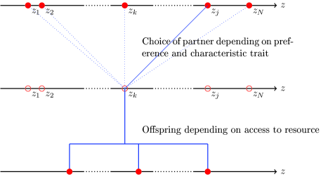
Figure 1. A pictorial description of the replicator dynamics of the population

More precisely

1. An individual $k$ has access to a fraction $\ c_{k}$ of the available resource:

   $$\ c_{k}=\int_{\mathcal{X}}\frac{e^{-(x_{k}-x)^{2}/2\sigma_{x}^{2}}}{\sum_{j=1}^{N_{t}}\int_{\mathcal{X}}e^{-(x_{j}-x)^{2}/2\sigma_{x}^{2}}}\,.\frac{df(x)}{\|f\|}$$

   This represents the competition among the individuals.

2. Each individual $k$ is given the opportunity to choose a mating partner, and chooses $j$ with probabilily

   $$\mbox{Prob}(j_{k}=j) = \left\{\begin{array}[]{ll}\frac{e^{-|y^{*}_{k}-y_{j}|^{2}/2\sigma^{2}}}{\sum_{i\neq k}e^{-|y^{*}_{k}-y_{i}|^{2}/2\sigma^{2}}}&\qquad(j\neq k)\,,\\ \\ 0&\qquad(k=j)\,.\end{array}\right.$$

   This is the reinforcement in the model, because it helps forming sub-populations such that mating takes place within the group. The parameter $\sigma$, which we have taken to be the same for all individuals in the population, determines the choosiness in selection of partners for mating.

3. The couple $(k,j_{k})$ then produces a Poisson distributed number $n_{\kappa}$ of children, with rate $\frac{c_{k}+c_{j_{k}}}{2}\|f\|$, i.e. proportional to the amount the the resource that has been collected by the couple. This means that the size of the population at time $t+1$ will be a Poisson distributed variable, $N_{t+1}=\sum_{k=1}n_{k}$ with a random parameter

   $$\lambda=\|f\|\left(1+\sum_{k=1}^{{}_{t}}c_{j_{k}}\right).$$

   It is random because of the random choice of partner, $j_{k}$, and the law depends on the whole population at time $t$.

4. Each child has a trait $z=z_{k,i}$, $i=1...n_{k}$

   $$z_{k,i} = \frac{z_{k}+z_{j_{k}}}{2}+(\xi_{i},\eta_{i},\eta^{*}_{i})\,.$$

   where $(\xi_{i},\eta_{i},\eta^{*}_{i})$ are Gaussian random variables.

Some simulation results are shown in Figure 2, 3 and 4. For the simulations in Figure 2, the food resource is concentrated at two points, $x=\pm 1$, and the population is initially monomorph with phenotype $x=0$. Without reinforcement, as in (a), the population remains concentrated around $x=0$ although the small mutations are seen as noise in the distribution. With reinforcement, as in (b), (c), and (d), the population immediately splits in two sub-populations, each one exploiting one of the food resources. The graph in (d) shows the distribution of the appearance trait $y$. It does also separate in two parts, but there is no reason for the parts to stay at any particular position, and therefore these will carry out a random walk in the $\mathcal{Y}$-space. Eventually the two branches could meet, which would lead to the appearance of hybrid phenotypes. The graph in (d) shows the evolution of the “food distribution entropy”,

$$W_{c}(t)=\sum_{k=1}^{N_{t}}c_{k}\log(N_{t}c_{k})\,,$$

which is zero if and only if $c_{k}=1/N_{t}$ for all $k$. The simulations show that the population approaches a situation where all individuals attract the same quantity of the food resource.

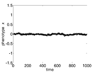
(a)

(b)

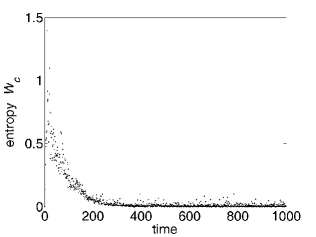
(c)

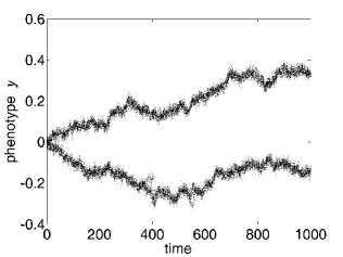
(d)

Figure 2. (a) and (b) $x$-trait without and with reinforcement.
(c) $c$-entropy, $W_{c}$, (d): appearance trait $y$

Figure 3 shows the results of a simulation where the food resources are equally distributed at the points $x=-1,0,1$, and as expected, with reinforcement, the population will then split in three sub-populations, but it may happen in different ways: The figures (a), (b), and (c), (d) show the results of two simulations with exactly the same initial conditions.

And then Figure 4, shows the result in which the food distribution is Gaussian in $x$, with mean zero, and the $x$-phenotype is initially concentrated at $x=2$. We can see in (a) how the whole population evolves to $x$-values close to zero, before the splitting into sub-populations take place. The graph in (c) shows the food distribution entropy, and the graph in (d) the size of the population, $N_{t}$.

(a)

(b)

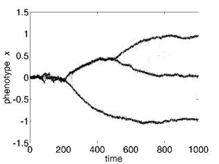
(c)

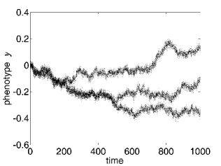
(d)

Figure 3. Two simulations with identical parameters.
(a) and (c): trait $x$ in the population, and (b) and (d): trait $y$.

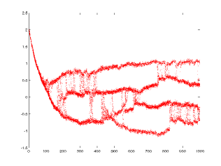
(a)

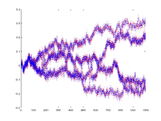
(b)

(c)

(d)

Figure 4. 100 individuals, Gaussian food distribution

The model can be reformulated into a more mathematically tractable form by identifying the population $Z_{t}$ by a point measure in $\mathcal{Z}$:

$$Z_{t}\leftrightarrow\sum_{j=1}^{\langle Z_{t},1\rangle}\delta_{z_{j}}\in\mathcal{M}_{P}(\mathcal{Z})\qquad(N_{t}=\langle Z_{t},1\rangle)\,.$$

To find an expression for $Z_{t+1}$, we write the offspring from an individual $z_{j}$ as

$$\Gamma\left(\cdot,z_{j}\right)=\sum_{i=1}^{\langle\Gamma\left(\cdot,z_{j}\right),1\rangle}\delta_{z_{i}}\qquad(\mbox{offspring from }z_{j})\,.$$

Then the next generation is

$$Z_{t+1}=\sum_{j=1}^{\langle Z_{t},1\rangle}\Gamma\left(\cdot,z_{j}\right)=\int_{\mathcal{Z}}\Gamma(\cdot,z)Z_{t}(dz)\,.$$

Here $\Gamma(\cdot,z)$ is a random point measure in $\mathcal{Z}$, whose law can be computed from the description above. The details are given in [28]. From this we wish to write a master equation for the process, to find a formula for

$$\mathbb{E}\left[\int_{\mathcal{Z}}\phi(z)Z_{t+1}(dz)\,\Bigg{|}\,Z_{t}\right]=\int_{\mathcal{Z}}{\mathbb{E}\left[\int_{\mathcal{Z}}\phi(z)\Gamma(dz,z^{\prime})\,\Bigg{|}\,Z_{t}\right]}Z_{t}(dz^{\prime})\,.$$

To continue, we first write $\Gamma$ by conditioning on the mating partner,

(2) $$\mathbb{E}\left[\int_{\mathcal{Z}}\phi(z)\Gamma(dz,z^{\prime})\,\Bigg{|}\,Z_{t}\right]=\int_{\mathcal{Z}}{\mathbb{E}\left[\int_{\mathcal{Z}}\phi(z)\Gamma(dz,z^{\prime})\,\Bigg{|}\,Z_{t},z^{\prime\prime}\right]}{P(z^{\prime},z^{\prime\prime})Z_{t}(dz^{\prime\prime})}\,,$$

where the choice of mating partner, $\mbox{Prob}(j_{k}=j)$, is encoded in

$$P(z^{\prime},z)=\frac{e^{-|y-y^{*}{}^{\prime}|^{2}/2\sigma^{2}}1\!\!1_{z\neq z^{\prime}}}{\int_{\mathcal{Z}}e^{-|y^{\prime\prime}-y^{*}{}^{\prime}|^{2}/2\sigma^{2}}1\!\!1_{z^{\prime\prime}\neq z^{\prime}}Z_{t}(dz^{\prime\prime})}\,.$$

The size of the offspring then depends on the resource distribution in the population,

$$c(z)=\int_{\mathcal{X}}\frac{e^{-(x-x^{\prime})^{2}/2\sigma_{x}^{2}}}{\int_{\mathcal{Z}}e^{-(x^{\prime\prime}-x^{\prime})^{2}/2\sigma_{x}^{2}}Z_{t}(dz^{\prime\prime})}\frac{f(dx^{\prime})}{\|f\|}\,.$$

The expectation value in the integral in the right-hand side of equation (2) can then be computed as as

$$\mathbb{E}\left[\int_{\mathcal{Z}}\phi(z)\Gamma(dz,z^{\prime})\,\Bigg{|}\,Z_{t},z^{\prime\prime}\right]=$$

$$= \sum_{k=0}^{\infty}{\mbox{Prob}[\langle\Gamma(dz,z^{\prime}),1\rangle=k\,|\,Z_{t},z^{\prime\prime}]}\times$$

$$\qquad\sum_{i=1}^{k}\int_{\mathcal{Z}}\phi\left(\frac{z^{\prime}+z^{\prime\prime}}{2}+\zeta_{i}\right)M(\zeta_{i})\,d\zeta_{i}.$$

The last sum gives the contribution from each child of parents with phenotype $z^{\prime}$ and $z^{\prime\prime}$; the phenotype of the child is the average of the parents’ phenotypes plus a random mutation $\zeta$ which is distributed with law $M(\zeta)d\zeta$. The number of offspring $k$ is Poisson distributed:

$$\mbox{Prob}[\langle\Gamma(dz,z^{\prime}),1\rangle=k\,|\,Z_{t},z^{\prime\prime}]=\frac{{\kappa(z^{\prime},z^{\prime\prime})}^{k}}{k!}e^{-{\kappa(z^{\prime},z^{\prime\prime})}}\,,$$

with

$$\kappa(z^{\prime},z^{\prime\prime})=\frac{c(z^{\prime})+c(z^{\prime\prime})}{2}\int_{\mathcal{X}}f(dx)\,.$$

In this form, the equations are still not very explicit, but one may formally take the limit of infinitely many individuals as in the paper by Méléard and Tran, as described above: we let $\mathcal{Z}_{t}^{n}=\frac{1}{n}\sum_{i=1}^{n\langle Z_{t}^{n},1\rangle}\delta_{(x_{i}(t),a_{i}(t))}$, and we assume that this has a limit as $n\rightarrow\infty$, and even that the limit is given by a density: $Z_{t}^{n}\rightarrow u_{t}(z)$ with $u_{t}=u_{t}(z)=u_{t}(x,y,y^{*})\in L^{1}(\mathcal{X}\times\mathcal{Y}\times\mathcal{Y}*)=L^{1}(\mathcal{Z})$,  $u\geq 0$, $t\in\mathbb{N}$.

It is then possible to identify the limiting expressions for the food distribution, the probability of choosing a particular mating partner, et.c.:

$$c_{k} \mapsto c(z;u)=\int_{\mathcal{X}}\frac{\displaystyle e^{-(x-x^{\prime})^{2}/2\sigma_{x}^{2}}}{\displaystyle\int_{\mathcal{Z}}e^{-(x^{\prime\prime}-x^{\prime})^{2}/2\sigma_{x}^{2}}u(z^{\prime\prime})\,dz^{\prime\prime}}df(x^{\prime})\,,$$

$$\mbox{Prob}(j_{k}=j) \mapsto \pi(z,z^{\prime};u)=\frac{e^{-|y^{*}-y^{\prime}|^{2}/2\sigma^{2}}}{\int_{\mathcal{Z}}e^{-|y^{*}-y^{\prime\prime}|^{2}/2\sigma^{2}}u(z^{\prime\prime})\,dz^{\prime\prime}}\,,$$

$$\kappa_{k} \mapsto \kappa(z,z^{\prime};u)=\frac{c(z;u)+c(z^{\prime};u)}{2}\int_{\mathcal{X}}df(x^{\prime})\,.$$

Finally we may write the master equation for the limiting densities $u_{n}$,

(3) $$\int_{\mathcal{Z}}\phi(z)u_{t+1}(z)\,dz=$$

$$= \int_{\mathcal{Z}}\int_{\mathcal{Z}}\int_{\mathcal{Z}}u_{t}(z^{\prime})u_{t}(z^{\prime\prime})\lambda(z^{\prime},z^{\prime\prime};u)P_{z^{\prime}}(z^{\prime\prime};u)M(z)\phi\left(\frac{z^{\prime}+z^{\prime\prime}}{2}+z\right)\,dz^{\prime}dz^{\prime\prime}dz$$

$$= \int_{\mathcal{Z}}\bigg{[}\int_{\mathcal{Z}}\int_{\mathcal{Z}}u_{t}(z^{\prime})u_{t}(z^{\prime\prime})\lambda(z^{\prime},z^{\prime\prime};u)\times$$

$$\hskip 100.00015ptP_{z^{\prime}}(z^{\prime\prime};u)M\left(z-\frac{z^{\prime}+z^{\prime\prime}}{2}\right)\,dwdz^{\prime\prime}\bigg{]}\phi(z)\,dz\,.$$

In the change of variables used to obtain the last line, it is assumed that $\mathcal{Z}={\mathbb{R}}^{d}$. To conclude, $u_{t+1}$ can be expressed in terms of $u_{t}$ using the expression in brackets in the last member of equation (3). However, I want to stress that this is only a very formal derivation, and also that there are no mathematical results concerning e.g. the long time behavior of the model.

2.4. An averaging process

If we neglect the rather complicated process of choosing the mating partner, the way in which the food resource is distributed, and how this affects the number of offspring of a given couple, the process is a simple one: according to some probability distribution, choose a random couple of individuals, and replace this couple by an offspring whose phenotype is the average of the parents’ but randomly displaced due to mutations. An extremely simplified version of this is the following:

Consider $N$ individuals with a scalar phenotype $x\in{\mathbb{R}}$. The population is therefore described by $(x_{1},...,x_{N})$. The phenotype distribution is then updated as follows:

• choose a couple $(x_{j},x_{k})$ uniformly at random

• replace those two individuals with a new couple, as

  $$(x_{j},x_{k})\mapsto\left(\frac{x_{j}+x_{k}}{2}+X_{1},\frac{x_{j}+x_{k}}{2}+X_{2}\right)\,,$$

  where $X_{1}$ and $X_{2}$ are i.i.d. with probability density $g(x)\in L^{1}({\mathbb{R}})$.

We now assume that in some limit all the $x_{i}$ are distributed with a law $f(x)dx$. If $x_{0}$ is drawn from this distribution, it should be the result of a replacement, i.e.

$$x_{0}=\frac{x_{1,1}+x_{1,2}}{2}+X_{0},$$

where also $x_{1,1}$ and $x_{1,2}$ are distributed with law $f(x)$, and where $X_{0}$ is a random variable with distribution $g(x)$. The same argument can be repeated for $x_{1,1}$ and $x_{1,2}$, which then gives (the notation should be clear)

$$x_{0} = \frac{1}{2}\left(\frac{x_{2,1}+x_{2,2}}{2}+X_{1,1}+\frac{x_{2,3}+x_{2,4}}{2}+X_{1,2}\right)+X_{0}$$

$$= \frac{1}{4}\left(x_{2,1}+x_{2,2}+x_{2,3}+x_{2,4}+x_{2,1}+x_{2,2}\right)+\frac{1}{2}\left(X_{1,1}+X_{1,2}\right)+X_{0}\,.$$

The procedure can be repeated, and after $n$ iterations we have

$$x_{0} = \frac{1}{2^{n}}\sum_{j=1}^{2^{n}}x_{n,j}$$

$$+\;\frac{1}{2^{n-1}}\sum_{j=1}^{2^{n-1}}X_{n-1,j}\;+\;...\;+$$

$$+\;\frac{1}{4}\sum_{j=1}^{4}X_{2,j}\;+\;\frac{1}{2}\left(X_{1,1}+X_{1,2}\right)\;+\;X_{0}\,.$$

By the law of large numbers, the first term converges to $\int_{{\mathbb{R}}}xf(x)\,dx$ when $n\rightarrow\infty$, and the other terms can be expressed exactly in terms of the distribution $g$: The law of $\frac{1}{2^{n-1}}\sum_{j=1}^{2^{n-1}}X_{n-1,j}$ is $2^{n-1}g^{*2^{n-1}}(2^{n-1}\cdot)$, for example. This gives a relation between the densities $f$ and $g$, which is most easily expressed in terms of their Fourier transforms:

$$\hat{f}(\xi) = \left(\frac{1}{2^{n}}\hat{f}\left(\frac{\xi}{2^{n}}\right)^{2^{n}}\right)\times$$

$$\left(\frac{1}{2^{n-1}}\hat{g}\left(\frac{\xi}{2^{n-1}}\right)^{2^{n-1}}\right)\cdots\left(\frac{1}{4}\hat{g}\left(\frac{\xi}{4}\right)^{4}\right)\left(\frac{1}{2}\hat{g}\left(\frac{\xi}{2}\right)^{2}\right)\hat{g}(\xi)\,.$$

If $f$ has bounded second moments, the first factor converges to 1 when $n\rightarrow\infty$ (this is obviously sufficient to guarantee that the law of large numbers holds), and we have then an explicit expression of $f$ in terms of the the distribution $g$. One example where this can be computed explicitly is when $g$ is a Gaussian function with variance $\sigma$; then $f$ will also be Gaussian, but with variance $2\sigma$.

We end this section by writing a master equation for the process, and computing expressions for the evolution of marginals. While this doesn’t have much to do with the model for speciation, it gives an introduction to much of what will follow. For a system of $N$ particles, the configuration space is ${\mathbb{R}}^{N}$ (there is no hardcore condition or similar restriction to the particle configuration). Let $f_{N}(x_{1},.....,x_{N})$ be a density in ${\mathbb{R}}^{N}$. One replacement according to description above, replacing a randomly chosen pair of particles by new particles whose position is the average of the parents’s position plus independent displacements, transforms the density as

(4) $$f_{N}(x_{1},.....,x_{N}) \mapsto \;f_{N}^{\prime}(x_{1},.....,x_{N})=$$

$$\quad\frac{2}{N(N-1)}\sum_{j<k}\int_{{\mathbb{R}}}\int_{{\mathbb{R}}}f_{N}(x_{1},...,x_{j}^{\prime},...,x_{k}^{\prime},...,x_{N})\times$$

$$\qquad\qquad g(x_{j}-\frac{x_{j}^{\prime}+x_{k}^{\prime}}{2})g(x_{k}-\frac{x_{j}^{\prime}+x_{k}^{\prime}}{2})\,dx_{j}^{\prime}dx_{k}^{\prime}$$

As is commonly done, we assume that the densities are symmetric with respect to permutation of the variables, and it is easy to see that if this holds for $f_{N}$, then it also holds for $f_{N}^{\prime}$: symmetry is preserved by the dynamics. The $k$-particle marginals are defined as

$$f_{N,k}(x_{1},...,x_{k})=\int_{{\mathbb{R}}^{N-k}}f_{N}(x_{1},...,x_{k},x_{k+1},...,x_{N})\,dx_{k+1}\cdots dx_{N}\,.$$

Because of the permutation symmetry, the same result would be obtained by leaving any set of $k$ variables untouched, integrating over the remaining $N-k$ variables. Integrating both sides of equation (4) over $k_{k+1},...,k_{N}$, we find an expression for how the $k$-particle marginals are transformed by the replacement process. For $k=1$ and $k=2$ the result is

$$f_{N,1}^{\prime}(x_{1})=\left(1-\frac{1}{N}\right)\left(1-\frac{1}{N-1}\right)f_{N,1}(x_{1})+$$

$$\qquad\qquad\frac{2}{N}\int_{{\mathbb{R}}}\int_{{\mathbb{R}}}f_{N,2}(x_{1}^{\prime},x_{2}^{\prime})g(x_{1}-\frac{x_{1}^{\prime}+x_{2}^{\prime}}{2})\,dx_{1}^{\prime}dx_{2}^{\prime}\,,$$

and

$$f_{N,2}^{\prime}(x_{1},x_{2})=\left(1-\frac{2}{N}\right)\left(1-\frac{2}{N-1}\right)f_{N,k}(x_{1},x_{2})+$$

$$\qquad\qquad\frac{2(N-2)}{N(N-1)}\int_{{\mathbb{R}}}\int_{{\mathbb{R}}}f_{N,3}(x_{1},x_{2}^{\prime},x_{3}^{\prime})g(x_{2}-\frac{x_{2}^{\prime}+x_{3}^{\prime}}{2})\,dx_{2}^{\prime}dx_{3}^{\prime}+$$

$$\qquad\qquad\frac{2(N-2)}{N(N-1)}\int_{{\mathbb{R}}}\int_{{\mathbb{R}}}f_{N,3}(x_{1}^{\prime},x_{2},x_{3}^{\prime})g(x_{1}-\frac{x_{1}^{\prime}+x_{3}^{\prime}}{2})\,dx_{1}^{\prime}dx_{3}^{\prime}+$$

$$\qquad\qquad\frac{2}{N(N-1)}\int_{{\mathbb{R}}}\int_{{\mathbb{R}}}f_{N,2}(x_{1}^{\prime},x_{2}^{\prime})g(x_{1}-\frac{x_{1}^{\prime}+x_{2}^{\prime}}{2})g(x_{2}-\frac{x_{1}^{\prime}+x_{2}^{\prime}}{2})\,dx_{1}^{\prime}dx_{2}^{\prime}\,.$$

respectively. Here, and in all higher order terms, we find that the expression for $f_{k}^{\prime}$ involves terms with $f_{k+1}$, so if $k<N$, the system will never be closed.

The next step is to let $N\rightarrow\infty$. For this to make sense, we write $f_{N,k}^{j}(v_{1},...,v_{k})$ the distribution obtained after $j$ replacements, and write

(5) $$\frac{f_{N,1}^{j+1}(x_{1})-f_{N,1}^{j}}{2/N}=\int_{{\mathbb{R}}}\int_{{\mathbb{R}}}f_{N,2}^{j}(x_{1}^{\prime},x_{2}^{\prime})g(x_{1}-\frac{x_{1}^{\prime}+x_{2}^{\prime}}{2})\,dx_{1}^{\prime}dx_{2}^{\prime}-f_{N,1}^{j}(x_{1})\,.$$

Now, if one thinks of $f_{N,k}^{j}$ as being the values of a time dependent function evaluated at discrete points, $f_{N,k}^{j}(v_{1},...,v_{k})=f_{N,k}(v_{1},...,v_{k},\Delta_{t}j)$ with $\Delta_{t}=2/N$, the left-hand side of equation (5) is a finite difference approximation of $\displaystyle\frac{\partial}{\partial t}f_{N,k}(v_{1},...,v_{k},\Delta_{t}j)$. Passing to the limit as $N\rightarrow\infty$ gives

$$\frac{\partial}{\partial t}f_{1}(x_{1},t)=\int_{{\mathbb{R}}}\int_{{\mathbb{R}}}f_{2}(x_{1}^{\prime},x_{2}^{\prime},t)g(x_{1}-\frac{x_{1}^{\prime}+x_{2}^{\prime}}{2})\,dx_{1}^{\prime}dx_{2}^{\prime}-f_{1}(x_{1},t)$$

If in addition we assume that propagation of chaos holds, that is, $f_{2}(x_{1}^{\prime},x_{2}^{\prime},t)=f_{1}(x_{1}^{\prime},t)f_{1}(x_{2}^{\prime},t)$ (this will be discussed at length in the following sections), then a closed equation for the one-particle marginal is obtained:

(6) $$\frac{\partial}{\partial t}f_{1}(x_{1},t)=\int_{{\mathbb{R}}}\int_{{\mathbb{R}}}f_{1}(x_{1}^{\prime},t)f_{1}(x_{2}^{\prime},t)g(x_{1}-\frac{x_{1}^{\prime}+x_{2}^{\prime}}{2})\,dx_{1}^{\prime}dx_{2}^{\prime}-f(x_{1},t)\,.$$

Similar equations can be obtained for all marginals, but if the proportion of chaos is assumed to hold, then all information is already present in equation (6).

3. Applications from biology: models of flocking animals

It is fascinating to watch the huge bird flocks flying over big cities, or schools of fish that are forming close to bridges, sometimes, and recently there have been many attempts to make mathematical models to describe the observed phenomena. What is intriguing is that these complex structures can be formed without any obvious leader, all individuals in the flock should have the same status. How can the presumably rather simple rules controlling the behavior of individual birds result in this complex collective behavior?

In the first section I will present a couple of well known mathematical models related to swarming animals (without any claim to give a comprehensive list), and then discuss a model which has been analyzed in [9] in some more detail.

3.1. The Boids and Cucker-Smale models

The boids model [40] is a system of ODEs describing the evolution of $N$ particles:

$$\mathbf{\ddot{r}}_{i} = \sum_{j}\Big{[}f(r_{i,j})\mathbf{\hat{r}}_{ij}+\alpha_{1}\langle\mathbf{v}_{j}-\mathbf{v}_{i}|r_{ij}<r_{c}\rangle$$

$$\quad+\alpha_{2}\langle\mathbf{r}_{j}-\mathbf{r}_{i}|r_{ij}<r_{c}\rangle\Big{]}-\gamma\mathbf{v}_{i}+\beta\mathbf{\zeta}_{i}\,.$$

Here $\mathbf{r}_{i}$ is the position of “boid” $j$. The different terms describe the boid’s desire to move towards the average position of swarm, to approach the average velocity of the boids within a smaller neighborhood, and to avoid crowding.

There are other models that are discrete in time, and the Cucker-Smale model [14] is a particular example for which much progress on the mathematical theory has been made recently [27]. Here the velocities $v_{i}(t)$, $i=1,...,N$, $t=1,2,3,...$ evolve according to

$$v_{i}(n+1)-v_{i}(n) = \frac{\gamma}{N}\sum_{j=1}^{N}a_{ij}\,,\left(v_{j}(n)-v_{i}(n)\right)$$

$$a_{i,j} = \frac{1}{(1+\|x_{i}-x_{j}\|^{2})^{\beta}}\,.$$

The main mechanism here is alignment, the particles strive to align with the surrounding particles, and the strength of interaction depends on the distance between the particles through the function $a_{i,j}$.

A Boltzmann equation inspired by the model of Cucker and Smale has been derived by Carillo et al. [12]. They consider a density of individuals, $f(x,v,t)$, interacting pairwise by exchanging velocities according to

$$v^{*} = (1-\gamma a(x-y))v+\gamma a(x-y)w$$

$$w^{*} = \gamma a(x-y)v+(1-\gamma a(x-y))w\,,$$

and this leads to a Boltzmann equation

$$\left(\frac{\partial}{\partial t}+v\cdot\nabla_{x}\right)f(x,v,t) = Q(f,f)(x,v,t)\,.$$

where the collision operator (the binary interactions) is

$$Q(f,f)(x,v) = \int_{\mathbb{R}^{3}}\int_{\mathbb{R}^{3}}\left(\frac{1}{J}f(x,v^{*})f(y,w^{*})-f(x,v)f(y,w)\right)\,dw\,dy$$

3.2. The Vicsec model and a related Boltzmann equation

A discrete time model somewhat similar to that of Cucker and Smale was derived by Vicsec [48, 15], and has since been used in a large number of publications. In this model, all velocities have the same magnitude, $v_{0}$, and the direction is updated in one of the following ways [13]:

(7) $$v_{i}(t+\Delta t)=v_{0}\theta\left[\sum_{j\in S_{i}}v_{j}(t)+\eta\mathcal{N}_{i}\xi\right]\,,$$

or

(8) $$v_{i}(t+\Delta t)=v_{0}\left(\mathcal{R}_{\eta}\circ\theta\right)\left[\sum_{j\in S_{i}}v_{j}(t)\right]\,.$$

In both these models, $S_{i}$ is the set of neighbors to the particle $i$, defined as all other particles in side a ball of given radius around $x_{i}$, the position of particle $i$. This means that particle $i$ only interacts with other particles inside this ball. The function $\theta[\cdot]$ normalizes a vector: $\theta(v)=v/|v|$. In (7) the new velocity of particle $i$ is computed by first taking the average velocity of the particles inside the radius of interaction, adding a random vector scaled by the number $N_{i}$ of particles inside the ball of interaction, and finally normalizing the magnitude. In (8) the new velocity is computed by first finding the average velocity of the particles in the ball (as in (7), normalizing and finally carrying out a random rotation $\mathcal{R}_{\eta}$. The two models have been analyzed carefully with respect to e.g. phase transitions in [13].

A Boltzmann equation related to the Vicsec model has been derived in [5]:

Figure 5. The velocity jumps in the model of Bertin et al.

$$\frac{\partial f}{\partial t}(r,\theta,t)+e(\theta)\cdot\nabla f(x,\theta,t)=-\lambda f(r,\theta,t)+\lambda\int_{-\pi}^{\pi}d\theta^{\prime}\int_{-\infty}^{\infty}d\eta p_{0}(\eta)\times$$

$$\hskip 142.26378pt\sum_{m=-\infty}^{\infty}\delta(\theta^{\prime}+\eta-\theta+2\pi m)f(r,\theta^{\prime},t)$$

$$-f(r,\theta,t)\int_{-\pi}^{\pi}d\theta^{\prime}|e(\theta^{\prime})-e(\theta)|f(r,\theta,t)$$

$$+\int_{-\pi}^{\pi}d\theta_{1}\int_{-\pi}^{\pi}d\theta_{2}\int_{-\infty}^{\infty}d\eta p(\eta)|e(\theta_{2})-e(\theta_{1})|f(r,\theta_{1},t)f(r,\theta_{2},t)$$

$$\hskip 142.26378pt\times\sum_{m=-\infty}^{\infty}\delta(\bar{\theta}+\eta-\theta+2\pi m)\,.$$

3.3. A simple kinetic equation on the circle

In order to derive fluid equations by the Hilbert or Chapman - Enskog methods, one needs to know the equilibrium distributions, and in order to approach this we will now study a simpler, spatially homogeneous model in the plane [9], which can be derived from a master equation very similar to the one in Section 2.4,

(9) $$\partial_{t}f(t,\theta) = \int_{-\pi}^{\pi}\int_{-\pi}^{\pi}\bigg{(}f(t,\theta^{\prime})f(t,\theta^{\prime}+\theta_{*})g(\theta-\theta^{\prime}-\frac{\theta_{*}}{2})$$

$$\quad\qquad-f(t,\theta)f(t,\theta+\theta_{*})\bigg{)}\beta(|\sin(\theta_{*}/2)|)\frac{d\theta^{\prime}}{2\pi}\frac{d\theta_{*}}{2\pi}\,,$$

which corresponds to a jump process as depicted in the rightmost part of figure 5: two particles with velocities $\theta_{1}$ and $\theta_{2}$ (so the velocities are represented by angles) get new velocities $\theta_{j}^{\prime}=\bar{\theta_{1,2}}+\theta_{j}^{\prime\prime}$, $j=1,2$. In this expression, $\theta_{1}^{\prime\prime}$ and $\theta_{2}^{\prime\prime}$ are two independent angles distributed with law $g(\theta)$. Note the similarity with the averaging process described in the previous section. The model is also very similar to the model of rod alignment in [4]. It is easy to see that, for all distributions $g$, the uniform distribution $f(\theta)=1/(2\pi)$ is a stationary solution, but it it may not be the only one. Equation (9) may be written in terms of the Fourier series of $f(t,\theta)$. With $f(t,\theta)=\sum_{k=-\infty}^{\infty}a_{k}(t)e^{ik\theta}$,

$$\frac{da_{k}}{dt} = \sum_{n}a_{k-n}a_{n}\left(\gamma_{k}\Gamma(n-k/2)-\Gamma(k)\right)\,,$$

where

$$\gamma_{k}=\int_{-\pi}^{\pi}g(\theta)\frac{d\theta}{2\pi}\qquad\quad\Gamma(z)=\frac{\sin(\pi z)}{\pi z}\,.$$

($\Gamma$ actually depends on the function $\beta$ in (9), as written here it corresponds to $\beta\equiv 1$). To study the linear stability of the uniform distribution, we write $f(t,\theta)=1+\varepsilon\sum_{k=-\infty}^{\infty}b_{k}(t)e^{ik\theta}$, and then

$$\frac{d}{dt}b_{k}(t)=b_{k}(t)\underbrace{\bigg{(}2\gamma_{k}\Gamma(k/2)-\Gamma(0)-\Gamma(k)\bigg{)}}_{\lambda_{k}}+\mathcal{O}(\varepsilon)\,.$$

We then see that up to order $\varepsilon$, the Fourier modes are decoupled, and hence the linear stability can established by checking the sign of $\lambda_{k}$. By a direct calculation it follows that $\lambda_{k}<0$ if $k\geq 2$, and therefore the stability depends on $\lambda_{1}$, which is negative if and only if $\gamma_{1}<\pi/4$. This in turn depends on $g(\theta)$. As an example we take any density $\rho(x)\in L^{1}({\mathbb{R}})$, and let.

$$g_{\tau}(y)=2\pi\sum_{j=-\infty}^{\infty}\frac{1}{\tau}\rho(\frac{y-2\pi j}{\tau})\quad\Rightarrow\quad\gamma_{k}=\hat{\rho}(\tau k)\,.$$

The parameter $\tau$ determines how concentrated $g$ is around $\theta=0$. Clearly, when $\tau\rightarrow 0$, $\gamma_{1}\rightarrow 1>\pi/4$, and therefore the first Fourier mode is unstable for sufficiently small $\tau$. A similar result can be found in [4].

4. Propagation of chaos

Boltzmann’s and Maxwell’s kinetic theory was derived from a physical point of view, and it would take a very long time before a mathematically satisfactory derivation was carried out by Lanford [33] for a hard ball gas. And up to date, a derivation valid over macroscopic intervals of time is essentially missing (see the notes by Pulvirenti for details about this [39].

Mark Kac [31] invented a Markov process that mimics an $N$-particle system, proposed a mathematically rigorous definition of propagation of chaos, and showed that his model satisfies this property. In the following sections, we will present Kac’s model, and his proof, and then follow through the steps of e.g. Grünbaum [26] towards an abstract theorem stating not only that a large class of Markov processes do propagate chaos according to the definition of Kac, but also give precise error bounds in terms of the number of particles, and a detailed information about the limiting equation. The results are proven in [38] and [37]. An important ingredient in the abstract formulation is the de Finetti (or Hewitt Savage) theorem, which is also presented in these notes, following the lectures by P.L. Lions [34].

4.1. Kac’s approach to the propagation of chaos

Kac’s model of an $N$-particle system is a jump process on the sphere in ${\mathbb{R}}^{N}$,

$$S^{N-1}(\sqrt{N}))=\left\{(v_{1},...,v_{N})\;\Bigg{|}\;\frac{1}{2}\left(v_{1}^{2}+...+v_{N}^{2}\right)=N\right\}\,.$$

Each coordinate represents the (one dimensional) velocity of a particle, and the radius is chosen so that the expected energy of a particle (with unit mass) is one. The particles suffer binary collisions, which are modeled as jumps involving two coordinates at a time: At exponentially distributed time intervals, two coordinates, say $v_{i}$ and $v_{j}$ are chosen uniformly, randomly, and they are given new velocities $v_{i}^{\prime}$ and $v_{j}^{\prime}$:

$$(v_{1},...,v_{i},...,v_{j},...v_{N})\mapsto(v_{1},...,v_{i}^{\prime},...,v_{j}^{\prime},...v_{N})\,.$$

The new velocities are obtained as a random rotation in ${\mathbb{R}}^{2}$: $\theta$ is chosen at random according to a law $\mu$, and then

$$(v_{i}^{\prime},v_{j}^{\prime})=(v_{i}\cos(\theta)-v_{j}\sin(\theta),v_{i}\sin(\theta)+v_{j}\cos(\theta))\,.$$

We will use the notation $V\mapsto V^{\prime}=R_{i,j}(\theta)V$. Clearly

$${v_{i}^{\prime}}^{2}+{v_{j}^{\prime}}^{2}=v_{i}^{2}+v_{j}^{2}\,,$$

and therefore this process preserves energy exactly. On the other hand, there is no conservation of momentum

$${v_{i}^{\prime}}+{v_{j}^{\prime}}\neq v_{i}+v_{j}\,.$$

With only one dimensional velocities only trivial collisions can satisfy both energy and momentum conservation.

The Markov process just described can equivalently be defined by a master equation, which describes the evolution of phase space density. Writing $V=(v_{1},...,v_{N})$, and $\psi(V,t)=\psi(v_{1},...,v_{N},t)$, we assume that the random, initial point of the Markov jump process is distributed with density $\psi_{0}(V)$. To have a concrete example, we assume that the law for the random rotations in a collision is $\mu(d\theta)=(2\pi)^{-1}d\theta$ (any bounded measure can be treated in the same way, but for singular measures, as in e.g. [41], one needs to be a little more careful). The density at time $t$, $\psi(V,t)$ then satisfies

(10) $$\partial_{t}\psi_{N}(V,t)=\frac{2}{N-1}\sum_{1\leq i<j\leq N}\frac{1}{2\pi}\int_{-\pi}^{\pi}\left(\psi_{N}\big{(}R_{ij}(\theta)V,t\big{)}-\psi_{N}(V,t)\right)\,d\theta\,.$$

The factor in front of the sum in the right hand side implies that the system jumps on average $N$ times per unit time, and because the coordinates are drawn independently, this means that each coordinate is changed approximately twice per unit time. This corresponds to the Boltzmann Grad scaling of a real particle system, because each particle should then on average suffer the same (finite) number of collisions per unit time, independently of the number $N$ of particles.

Because all particles in a gas are assumed to be identical, the probability distribution of initial values should not depend on in which order we write them, and this is expressed by saying that the initial distribution should be symmetric with respect to permutations:

Definition 4.1.

The density $\psi_{0}(v_{1},...,v_{N})$ is symmetric if for any pair of variables, $v_{i},v_{j}$,

$$P[(v_{1},...,{v_{i}},...,{v_{j}},...,v_{N})\in A]=P[(v_{1},...,{v_{j}},...,{v_{i}},...,v_{N})\in A]\,.$$

The space of configurations obtained by identifying all points $V=(v_{1},...,v_{N})$ that can be obtained from each other by a permutation of the indices,

$$(v_{1},...,{v_{i}},...,{v_{j}},...,v_{N})\sim(v_{1},...,{v_{j}},...,{v_{i}},...,v_{N})\,,$$

is denoted $S^{N-1}(\sqrt{N}))/\mathfrak{S}_{N}$.

Note that the Kac jump process preserves permutation symmetry.

In the same way as the Kac master equation corresponds to the Liouville equation for a real $N$ particle system, there is a Boltzmann equation for the velocity distribution of one particle, that can formally be obtained in the limit of infinitely many particles. This is Kac’s caricature of the Boltzmann equation , the Kac equation:

(11) $$\partial_{t}f(v,t)=\int_{-\infty}^{\infty}\int_{-\pi}^{\pi}\left(f(v^{\prime},t)f(t,w^{\prime})-f(v,t)f(w,t)\right)\frac{d\theta}{2\pi}dw\,,$$

where just as in the definition of the jump process,

$$(v^{\prime},w^{\prime})=(v\cos(\theta)-w\sin(\theta),v\sin(\theta)+w\cos(\theta))\,.$$

In spite of its relative simplicity, its structure is very similar to that of the Boltzmann equation, and the two equations share many characteristics. There are numerous studies that consider the trend to equilibrium, tne regularity of solutions, its behavior in the presence of external force terms, … , with the hope that it will give insight into the behavior of the the full equation. Some relevant references are [18, 23, 3, 10].

Mass and energy conservation are among the most important properties of the solutions of the Kac equation:

$$\int_{{\mathbb{R}}}f(v,t)\,dv = const\,,$$

$$\int_{{\mathbb{R}}}f(v,t)v^{2}\,dv = const,$$

and also entropy $\int f\log fdv$ is non-increasing, just as for the real Boltzmann equation. On the other hand, the momentum is not a conserved quantity.

The master equation and the Kac equation are connected through the marginal distributions. We define, for $k=1\cdots N-1$,

$$f^{N}_{k}(v_{1},v_{2},...,v_{k},t)=\int_{\Omega_{k}}\psi_{N}(v_{1},...,v_{k},v_{k+1},...,v_{N},t)d\sigma_{k}\,,$$

where $\Omega_{k}=S^{N-1-k}\left(\sqrt{N-v_{1}^{2}-...-v_{k}^{2}}\right)$, and $\sigma_{k}$ is the uniform normalized measure on $\Omega_{k}$. The marginals $f^{N}_{k}$, the “k-particle distributions” give the distribution of one of the first $k$ coordinates, and because of the permutation symmetry, the distribution of any collection of $k$ different coordinates is the same, and correspond to the joint distribution of $k$ randomly chosen particles in a real gas. Because $\psi_{N}$ is assumed to be symmetric, the marginal distributions are too.

The evolution equations for the $k$-particle marginal can be obtained simply by integrating the master equation over $v_{k+1}\ldots v_{N}$. For example,

(12) $$\partial_{t}f^{N}_{1}(v_{1},t)=\int_{-\sqrt{N-v_{1}^{2}}}^{\sqrt{N-v_{1}^{2}}}\int_{-\pi}^{\pi}\left(f_{2}^{N}(v_{1}^{\prime},v_{2}^{\prime},t)-f_{2}^{N}(v_{1},v_{2},t)\right)\frac{d\theta}{2\pi}\,dv_{2}\,,$$

and similar equations can be obtained for all $f^{N}_{k}$. If we assume that for each $k$, $f^{N}_{k}\rightarrow f_{k}$ for some function $f_{k}(v_{1},...,v_{k},t)$, which for each $t$ is a density in ${\mathbb{R}}^{k}$, then it is possible, at least formally, to pass to the limit in (12) to get

(13) $$\partial_{t}f_{1}(v_{1},t)=\int_{-\infty}^{\infty}\int_{-\pi}^{\pi}\left(f_{2}(v_{1}^{\prime},v_{2}^{\prime},t)-f_{2}(v_{1},v_{2},t)\right)\frac{d\theta}{2\pi}\,dv_{2}\,.$$

The situation is similar for all $f_{k}$: because the right-hand side involves $f_{k+1}$, one does not obtain a closed system of equations. The whole discussion about propagation of chaos aims at proving that if certain hypotheses are satisfied, then $f_{k}(v_{1},...,v_{k},t)=f_{1}(v_{1},t)\cdot\ldots\cdot f_{1}(v_{k},t)$. The interpretation of this is that drawing a $k$-tuple of velocities is the same as drawing $k$ velocities independently, the particle velocities are independent. This cannot be true for any finite $N$, but can sometimes be proven to be correct in the limit as $N\rightarrow\infty$.

4.2. Propagation of chaos in Kac’s model

Kac defined propagation of chaos as follows:

Definition 4.2.

A sequence of probability measures $\psi_{N}(v_{1},...,v_{N})$, $N=1,...,\infty$ is said to have the Boltzmann property, or to be $chaotic$ if for each $k$,

$$\lim_{n\rightarrow\infty}f_{k}^{N}(v_{1},...,v_{k})\rightarrow\prod_{j=1}^{k}\lim_{n\rightarrow\infty}f_{1}^{N}(v_{j},t)\,.$$

Assume that the evolution of a sequence of probability measures $\psi_{N}(v_{1},...,v_{N},t)$ is governed by a family of Markov processes, and that the sequence is chaotic for each $t\geq 0$. Then the propagation of chaos is said to hold for these Markov processes.

One of the main achievements in [31] was Kac’s proof that propagation of chaos holds for his model, and hence that the Kac equation can be derived rigorously as the limit of a many particle system.

Theorem 4.3 (M. Kac).

Propagation of chaos holds for the master equation (10).

Very briefly, the main steps of the proof are as follows: Seen as an operator in $L^{2}(S^{N-1}(\sqrt{N}))$.

$$Q\psi_{N}(V)=\frac{2}{N-1}\sum_{1\leq i<j\leq N}\frac{1}{2\pi}\int_{-\pi}^{\pi}\left(\psi_{N}\big{(}R_{ij}(\theta)V\big{)}-\psi_{N}(V)\right)\,d\theta$$

is self adjoint and bounded,and hence $\psi_{N}(V,t)=\exp(tQ)\psi_{N}(V,0)$, where

(14) $$\psi_{N}(V,t)=\sum_{k=0}^{\infty}\frac{t^{k}}{k!}Q^{k}\psi_{N}(V,0)\,.$$

We then need to compute powers of $Q$. Consider first a bounded function $g_{1}(V)=g(v_{1})$, i.e. a function depending on only the first component of $V$, and let

(15) $$g_{2}(V)=g_{2}(v_{1},v_{2})=\int_{-\pi}^{\pi}(g_{1}(v_{1}\cos(\theta)+v_{2}\sin(\theta))-g_{1}(v_{1}))\frac{d\theta}{2\pi}\,.$$

By recursion, let

(16) $$g_{k+1}(v_{1},...,v_{k},v_{k+1})=$$

$$\sum_{j=1}^{k}\int_{-\pi}^{\pi}(g_{k}(v_{1},...,v_{j}\cos(\theta)+v_{k+1}\sin(\theta),...,v_{k})-g_{k}(v_{1},...,v_{k}))\frac{d\theta}{2\pi}\,.$$

The reason for introducing the $g_{k}$ in this way is that computing $\int_{S^{N-1}(\sqrt{N})}\psi_{N}(V)g_{1}(V)$ for all bounded $g_{1}(V)$ is enough to identify the one particle marginal $f^{N}_{1}(v_{1})$, and that because $Q$ is self adjoint, $\langle Q\Psi,g_{1}\rangle=\langle\Psi,Qg_{1}\rangle$. The formulae (15,16) then appear in the calculation of $\langle\Psi,Q^{k}g_{1}\rangle$.

Next we assume that the initial data are chaotic, so that $\psi_{N}(v_{1},...,v_{N},0)=f_{0,k}^{N}(v_{1},...,v_{N})$, and that there are functions $f_{0,k}$ such that $f_{0,k}(v_{1},...,v_{k})=$
$\lim_{N\rightarrow\infty}f_{0,k}^{N}(v_{1},...,v_{k})$, and moreover

$$\int_{-\infty}^{\infty}...\int_{-\infty}^{\infty}f_{k+1}(v_{1},...,v_{k+1})g_{k+1}(v_{1},...,v_{k+1})dv_{1}...dv_{k+1}$$

$$= \int_{-\infty}^{\infty}...\int_{-\infty}^{\infty}f_{1}(v_{1})\cdots f_{1}(v_{k+1})g_{k+1}(v_{1},...,v_{k+1})dv_{1}...dv_{k+1}\,.$$

Multiplying all terms in (14) with $g_{1}(v_{1})$, integrating and letting $N\rightarrow\infty$, we get

(17) $$\int_{-\infty}^{\infty}f_{1}(v_{1},t)g(v_{1})\,dv_{1}=$$

$$\sum_{k=0}^{\infty}\frac{t^{k}}{k!}\int_{-\infty}^{\infty}...\int_{-\infty}^{\infty}f_{0}(v_{1})\cdots f_{0}(v_{k+1})g_{k+1}(v_{1},...,v_{k+1})dv_{1},...,dv_{k+1}$$

for $0\leq t<2$. Similarly for the two-particle marginals

(18) $$\int_{-\infty}^{\infty}\int_{-\infty}^{\infty}f_{2}(v_{1},v_{2},t)g(v_{1})h_{(}v_{2})\,dv_{1}dv_{2}=$$

$$\sum_{k=0}^{\infty}\frac{t^{k}}{k!}\int_{-\infty}^{\infty}...\int_{-\infty}^{\infty}f_{0}(v_{1})\cdots f_{0}(v_{k+2})\gamma_{k+2}(v_{1},...,v_{k+2})dv_{1},...,dv_{k+2}\,.$$

Here the $\gamma_{k}$ are obtained by iteration:

$$\gamma_{2}(v_{2},v_{2}) = g(v_{1})h(v_{2})$$

$$\gamma_{k+1} = \sum_{j=1}^{k}\int_{-\pi}^{\pi}(\gamma_{k}(v_{1},...,v_{j}\cos(\theta)+v_{k+1}\sin(\theta),...,v_{k})-\gamma_{k}(v_{1},...,v_{j},...,v_{k}))d\theta\,.$$

We then need to prove that

$$\int_{-\infty}^{\infty}\int_{-\infty}^{\infty}f_{2}(v_{1},v_{2}t)g(v_{1})h_{(}v_{2})\,dv_{1}dv_{2}=\int_{-\infty}^{\infty}f_{0}(v_{1},t)g(v_{1})\,dv_{1}\int_{-\infty}^{\infty}f_{0}(v_{2},t)h(v_{2})\,dv_{2}\,.$$

This is done by proving that the series (17) and (18) are convergent, and by comparing the terms. This involves expressions like

$$\gamma_{3}(v_{1},v_{2},v_{3}) = g_{2}(v_{1},v_{3})h_{1}(v_{2})+g_{1}(v_{1})h_{2}(v_{2},v_{3})$$

$$\gamma_{4}(v_{1},v_{2},v_{3},v_{4}) = g_{2}(v_{1},v_{3})h_{2}(v_{2},v_{4})+g_{3}(v_{1},v_{3},v_{4})h_{1}(v_{2})$$

$$+g_{2}(v_{1},v_{4})h_{2}(v_{2},v_{3})+g_{1}(v_{1})h_{3}(v_{2},v_{3},v_{4})\,.$$

As for the convergence of the series, this turns out to hold of a bounded time interval, but this interval can be uniformly estimated, and hence one can prove that propagation of chaos holds for any bounded time interval.

4.3. Existence of chaotic states

Kac proved that there is a large class of functions distributions defined as

$$\psi_{N}(v_{1},...,v_{N}) = \frac{\prod_{j=1}^{N}c(v_{j})}{{\displaystyle\int\limits_{S^{N-1}(\sqrt{N})}}\;\prod_{j=1}^{N}c(w_{j})\;d\sigma_{N}(w_{1},...,w_{N})}\,.$$

The easiest examples are the uniform distributions, which are also the equilibria for the Kac master equations. If $\psi_{N}(V,t)$ is the solution to equation (10), then

$$\lim_{t\rightarrow\infty}\psi_{N}(V,t)=\frac{1}{|S^{N-1}(\sqrt{N})|}\,.$$

In this case one can carry out explicit calculations rather easily: To compute the limit of a one-particle marginal, let

$$P(v_{N}>w)=\left\{\begin{array}[]{ll}0&\mbox{ if }w>\sqrt{N}\\ \\ {\displaystyle\int_{v_{N}>w}}d\sigma_{N}(v_{1},...,v_{N})&\mbox{ if }-\sqrt{N}<w<\sqrt{N}\\ \\ 1&\mbox{ if }w<-\sqrt{N}\end{array}\right.$$

Then write the spherical cap as

$$Y_{\sqrt{N},w} = \left\{(v_{1},v_{2},...,v_{N});v_{1}^{2}+v_{2}^{2}+...+v_{N}^{2}=\sqrt{N}^{2},v_{N}\geq w\right\}\,,$$

whose area is

$$\mu(Y_{\sqrt{N},w}) = \mu(S^{N-1}(1))N^{(N-1)/2}\int_{0}^{\arccos(w/\sqrt{N})}(1-\cos^{2}(\theta))^{(N-3)/2}\sin{\theta}\,d\theta$$

$$= \mu(S^{N-1}(1))N^{(N-1)/2}\int_{w/\sqrt{N}}^{1}(1-x^{2})^{(N-3)/2}\,dx\,.$$

Finally, because

$$\sqrt{(N-3)/2}\int_{w/\sqrt{N}}^{1}(1-x^{2})^{(N-3)/2}\,dx \rightarrow \int_{w/\sqrt{2}}e^{-x^{2}}\,dx$$

we may deduce that the one-particle distribution converges to a Maxwellian, and a similar calculation can be carried out for the two-particle distribution, and so on.

5. Empirical distributions

One difficulty with the approach of Kac is that each $N$-particle system has its own state space, while the questions of convergence would be more easily stated if one could embed all the $N$-particle systems in the same space. One approach to this was suggested by Grünbaum [26], who proposed method for proving a propagation of chaos result for the spatially homogeneous Boltzmann equation for hard spheres. We begin by discussing this in abstract terms.

The phase space, or configuration space, for the $N$-particles is then $E^{N}$, an $N$-fold product of a Euclidean space $E$, or more precisly, in order that the way in which the particles are numbered is not important, $E^{N}/\mathfrak{S}_{N}$, the quotient group of $E^{N}$ with the symmetric group of $N$ elements. That means that

$$X=(x_{1},...,x_{N})\in E^{N}\mbox{ and }\tilde{X}=(\tilde{x}_{1},...,\tilde{x}_{N})\in E^{N}$$

are identified if $\tilde{X}$ can be obtained by a permutation of the coordinates of $X$. We then define the empirical measure associated with $X$ as

$$\hat{\mu}_{X}=\frac{1}{N}\sum\limits_{j=1}^{N}\delta_{x_{j}}\in{\mathcal{P}}_{N}(E)\subset{\mathcal{P}}(E)\,.$$

Here we have introduced the notation ${\mathcal{P}}(E)$ for the set of probability measures on $E$, and ${\mathcal{P}}_{N}(E)$ for the probability measures consisting of $N$ Dirac measures of equal mass. This is slightly at variance with the usual definition of empirical measure in probability theory, where the $x_{j}$ are assumed to be i.i.d. random variables with some distribution $\mu\in{\mathcal{P}}(E)$.

One important property of ${\mathcal{P}}(E)$ is that it is metrizable. Metrics can be introduced in several different ways, two of the most commonly used metrics being Lévy-Prokhorov metric, and Wasserstein distance. The first of these is defined as follows: Let $(E,d)$ be a metric space, and let ${\mathcal{P}}(E)$ the collection of probability measures on $E$. For $\mu,\nu\in{\mathcal{P}}(E)$,

$${\mathrm{d}_{LP}}(\mu,\nu)=\inf\left\{\varepsilon>0\,|\,\mu(A)<\nu(A^{\varepsilon})+\varepsilon\mbox{ and }\nu(A)<\mu(A^{\varepsilon})+\varepsilon\mbox{ for all }A\in{\mathcal{B}}(E)\right\}\,,$$

where $A^{\varepsilon}=\{x\in E\,\mbox{ such that }\inf_{y\in A}d(x,y)\leq\varepsilon\}$.

This definition depends, of course, on the metric $d$ on $E$. Given a distance on $E$, there is a natural way of introducing a distance on $E^{N}/\mathfrak{S}_{N}$. Let $X=(x_{1},...,x_{N})$, $Y=(y_{1},...,y_{N})\in E^{N}/\mathfrak{S}_{N}$. Then

$${\mathrm{d}_{LP}}(X,Y)=\inf_{\sigma\in\mathfrak{S}_{N},\varepsilon>0}\left\{\frac{\sharp\left\{i\;|\;|x_{i}-y_{\sigma_{i}}|>\varepsilon\right\}}{N}<\varepsilon\right\}\,.$$

And with this metric, we may then define the Levy-Prokhorov distance on ${\mathcal{M}}(E^{N}/\mathfrak{S}_{N})$. Note that this metric scales well with $N$. For example, if $X=(x,x,x,....,x)$ (i.e. $N$ copies of the same $x\in E$) and $Y=(0,....,0)$, then ${\mathrm{d}_{LP}}(X,Y)=|x|$, independently of $N$. On the other hand, if $X=(x_{1},0,...,0)$, then we always have ${\mathrm{d}_{LP}}(X,Y)\leq 1/N$.

As for the Wasserstein distance, it is defined as follows: Let $\Gamma(\mu,\nu)$ be the collection of $\gamma\in{\mathcal{P}}(E\times E)$ such that $\mu=\int_{E}\gamma(\cdot,dy)$ and $\nu=\int_{E}\gamma(dx,\cdot)$. Hence the $\gamma$s are are joint probability measures with $\mu$ and $\mu$ as marginal distributions, and the Wasserstein distance is defined as

$$W_{p}(\mu,\nu)^{p}=\inf\limits_{\gamma\in\Gamma(\mu,\nu)}\int_{E\times E}d(x,y)^{p}\,d\gamma(x,y)=\inf{\mathrm{E}}\left[|X-Y|^{p}\right]\,.$$

5.1. The Hewitt-Savage theorem

Hewitt-Savage theorem (which is an extension of de Finetti’s theorem) that is the topic of this section, is relevant for the discussion of propagation of chaos, but it is included here also to serve as an introduction to the rather abstract notation that will be used later. The material is essentially taken from [34].

Let $\mu^{N}\in{\mathcal{P}}(E^{N}/\mathfrak{S}_{N})$. The marginals $\mu_{k}^{N}\in{\mathcal{P}}(E^{k}/\mathfrak{S}_{N})$ are defined by

$$\int_{E^{k}}\phi(x_{1},...,x_{k})\mu_{k}^{N}(dx_{1},...,dx_{k})=\int_{E^{N}}\phi(x_{1},...,x_{k})\mu^{N}(dx_{1},...,dx_{k},...dx_{N})\,,$$

which should hold for every symmetric $\phi\in{\mathcal{C}}(E^{k})$. In the following we assume that $E$ is a compact metric space, but for example $E={\mathbb{R}}^{n}$ could be treated in a similar manner, although with some extra technical complication.

We then identify $X\in E^{N}/\mathfrak{S}_{N}$ with an empirical measure as above,

$$\hat{\mu}_{X}=\frac{1}{N}\sum_{k=1}^{N}\delta_{x_{k}}\in{\mathcal{P}}_{N}(E)\subset{\mathcal{P}}(E)\,,$$

this then yields a natural identification of functions $u:E^{N}/\mathfrak{S}_{N}\rightarrow{\mathbb{R}}$ with functions $\ {\mathcal{P}}_{N}(E)\rightarrow{\mathbb{R}}$:

$$u(X)\leftrightarrow u\left(\frac{1}{N}\sum_{j=1}^{N}\delta_{x_{j}}\right)\,.$$

Note that if this identification does not automatically preserve properties like continuity, unless som care is taken in chosing the metric on ${\mathcal{P}}(E^{k}/\mathfrak{S}_{N})$. The Levy-Prokhorov example given above has this property.

Next we consider a sequence of functions $\left\{u_{N}:E^{N}/\mathfrak{S}_{N}\rightarrow{\mathbb{R}}\right\}_{N=1}^{\infty}$. These are all defined on different spaces, and hence there is no immediate way of comparing the functions, and talking about convergence, et.c.. But the identification with measures in ${\mathcal{P}}(E)$ provides a mean of doing so: one can say that the sequence $u_{N}$ converges if the corresponding sequence of measures converges.

We have the follwing compactness result:

Consider a bounded sequence $\left\{u_{N}:E^{N}/\mathfrak{S}_{N}\rightarrow{\mathbb{R}}\right\}$ , with $|u_{N}|\leq C$, and let $\omega:{\mathbb{R}}^{+}\rightarrow{\mathbb{R}}^{+}$ be a strictly decreasing function with $\omega(r)\xrightarrow[r\rightarrow 0]{}0$. Assume that

$$\left|u_{N}(X)-u_{N}(Y)\right|\leq\omega({\mathrm{d}_{LP}}(X,Y))\,.$$

What this says is that the sequence is bounded and uniformly continuous with modulus of continuity $\omega$. Then there is a subsequence $u_{N^{\prime}}$ and $U\in{\mathcal{C}}({\mathcal{P}}(E))$ such that

$$\left\|u_{N^{\prime}}(x_{1},...,x_{N^{\prime}})-U\left(\frac{1}{N^{\prime}}\sum_{j=1}^{N^{\prime}}\delta_{x_{j}}\right)\right\|\rightarrow 0\,.$$

Of course, in most cases the limiting measure cannot be identified with any function $u_{N}:E^{N}/\mathfrak{S}_{N}\rightarrow{\mathbb{R}}$ for a finite value of $N$, but would are in all cases good examples of symmetric functions of infinitely many variables $x_{i}\in E$.

Next consider the following calculation: with $E$ compact, let $\mu^{N}\in{\mathcal{P}}(E^{N}/\mathfrak{S}_{N})$, $N=1,2,3....$, and consider the marginal distributions $\mu^{N}_{k}=\int\mu^{N}(\cdot,...,dx_{k+1},...,dx_{N})\in{\mathcal{P}}(E^{k}/\mathfrak{S}_{k})$, for $1\leq k<N$. Because $E$ is compact, ${\mathcal{P}}(E^{k}/\mathfrak{S}_{k})$ is also compact, and for every $k$ there is a subsequence $(N^{\prime})$ such that

$$\mu^{N^{\prime}}_{k}\rightarrow\mu_{k}\in{\mathcal{P}}(E^{k}/\mathfrak{S}_{k})\,.$$

By the usual diagonal procedure, it is then possible to extract a subsequence $N^{\prime\prime}$ such that

$$\mu^{N^{\prime\prime}}_{k}\rightarrow\mu_{k}\in{\mathcal{P}}(E^{k}/\mathfrak{S}_{k})\;\;\mbox{\color[rgb]{0,0,0} for all }\;\;k\,.$$

By construction, the $(\mu_{k})_{k=1}^{\infty}$ satisfy

(20) $$\mu_{k}=\int_{E}\mu_{k+1}(\cdot,dx_{k+1})\,.$$

The Hewitt-Savage theorem [29], which is a generalization of a theorem by de Finetti, concerns sequences of measures with exactly this property. It is common to express this as exchangability: a sequence of random variables, $X_{1},X_{2},....$ is said to be exchangeable if for any $n\geq 1$ and any $\sigma=(\sigma_{1},...,\sigma_{n})\in\mathfrak{S}_{n}$, the $n$-tuples $X_{1},...,X_{n}$ and $X_{\sigma_{1}},...,X_{\sigma_{n}}$ have the same distribution.

Theorem 5.1.

Assume that a sequence of measures $\mu_{k}\in{\mathcal{P}}(E^{k}/\mathfrak{S}_{N}),\;\;k=1,2...$ satisfies (20). There is $\pi\in{\mathcal{P}}({\mathcal{P}}(E))$ such that for all $k\geq 1$,

$$\mu_{k}(dx_{1},...,dx_{k})={\int}\prod_{i=1}^{k}m(dx_{i})\,\pi(dm)\,.$$

The easiest conceivable example, $\pi=\delta_{\bar{m}},\quad\bar{m}\in{\mathcal{P}}(E)$. Then $\pi$ is a measure on ${\mathcal{P}}({\mathcal{P}}(E))$ that is concentrated on $\bar{m}\in{\mathcal{P}}(E)$, and

$$\mu_{k}(dx_{1},...,dx_{k})={\int}\prod_{i=1}^{k}m(dx_{i})\,\delta_{\bar{m}}(dm)=\bar{m}(dx_{1})\cdots\bar{m}(dx_{k})\,.$$

That is: if $\pi$ is concentrated in one point $\bar{m}$, the measures derived from $\pi$ factorize.

Proof of theorem 5.1 (P.L. Lions) [34]: With $E$ compact, ${\mathcal{P}}(E)$ is a compact metric space, and we have constructed functions $U\in C({\mathcal{P}}(E))$. One can also define polynomials on ${\mathcal{P}}(E)$, and these obviously also belong to $C({\mathcal{P}}(E))$. The constants, polynomials of degree zero, are in $C({\mathcal{P}}(E))$, and to define polynomials of degree 1, take $\phi\in{\mathcal{C}}(E)$, and let

$$m\mapsto\int_{E}\phi(x)m(dx)\equiv P_{1}(m)\,.$$

If $m_{1}\neq m_{2}$, one can find $\phi$ such that $\int_{E}\phi(x)m_{1}(dx)\neq\int_{E}\phi(x)m_{2}(dx)$, and hence these linear functions separate points in ${\mathcal{P}}(E)$. Then the monomials $P_{j}(m)$ of degree $j$ are defined as follows. Take $\phi_{j}\in{\mathcal{C}}(E^{j}/\mathfrak{S}_{N})$ and then let

$$P_{j}(m)=\int_{E^{j}}\phi_{j}(x_{1},...,x_{j})m(dx_{1})\cdots m(dx_{j})\,.$$

From these definitions one may then define polynomials of all orders, and the Stone-Weierstrass theorem states that the set of polynomials is dense in $C({\mathcal{P}}(E))$. Evaluating these polynomials on empirical measures $m=\frac{1}{k}\sum_{j=1}^{k}\delta_{x_{j}}$, we find

$$P_{j}(m) = \int_{E^{j}}\phi_{j}(y_{1},...,y_{j})\left(\frac{1}{k}\sum_{i=1}^{k}\delta_{dx_{i}}(dy_{1})\right)\cdots\left(\frac{1}{k}\sum_{i=1}^{k}\delta_{dx_{i}}(dy_{j})\right)$$

$$= \frac{1}{k^{j}}\sum_{i_{1}=1}^{k}\cdots\sum_{i_{j}=1}^{k}\phi_{j}(x_{i_{1}},...,x_{i_{j}})+..$$

For example,

$$P_{2}\left(\frac{1}{3}(\delta_{x_{1}}+\delta_{x_{2}}+\delta_{x_{3}})\right)=\frac{1}{9}\sum_{i,j=1}^{3}\phi(x_{i},x_{j})\,.$$

In these second degree polynomials there are some terms like $\frac{1}{9}\phi(x_{1},x_{1})$, and the same will happen for polynomials of higher degree. However, when $k$ is much larger than the degree $j$ of the polynomial, a vast majority of the terms will be of the form $\phi(x_{i_{1}},...,x_{i_{j}})$ where all the arguments are different.

Now let $\{\mu_{k}\}_{k=1}^{\infty}$ be the measures given in the statement of the theorem, and consider

$$\int P_{j}\left(\frac{1}{k}\sum_{j=1}^{k}\delta_{x_{j}}\right)\mu_{k}(dx_{1},...,dx_{k})\approx\int\phi(x_{1},...,x_{j})\mu_{k}(dx_{1},...,dx_{j},...dx_{k})\,.$$

The difference between the left and right terms is due to the presence of terms with two or more of the arguments of $\phi$ are taken to be the same $x_{i}$, and so vanishes when $k$ is large compared to $j$. The error can be estimated by a simple combinatorial argument. And

$$\int\phi(x_{1},...,x_{j})\mu_{k}(dx_{1},...,dx_{j},...dx_{k})=\int\phi(x_{1},...,x_{j})\mu_{j}(dx_{1},...,dx_{j})$$

because of the relation (20).

Next we define a linear functional on the set of polynomials $P\in{\mathcal{C}}({\mathcal{P}}(E))$ by setting

$$\ell(P)=\lim_{k\rightarrow\infty}\int_{E^{k}}P\left(\sum_{j=1}^{k}\delta_{x_{j}}\right)\mu_{k}(dx_{1},...,dx_{k})$$

Then $P\mapsto\ell(P)$ is positive and $\ell(1)=1$, so $\ell$ is a positive, bounded functional defined on a dense subset of ${\mathcal{C}}({\mathcal{P}}(E))$, and can be extended to all of ${\mathcal{C}}({\mathcal{P}}(E))$. Then Riesz’s theorem states that there is a measure $\pi\in{\mathcal{P}}({\mathcal{P}}(E))$ such that

$$\ell(U)=\int_{{\mathcal{P}}(E)}U(m)\;\pi(dm)\,.$$

This measure, $\pi$ is the the desired measure. We only need to check that the measures $\mu_{k}$ can be obtained from $\pi$ as stated in the theorem. To this end, consider

$$\int_{{\mathcal{P}}(E)}\prod_{i=1}^{k}m(dx_{i})\,\pi(dm)\in{\mathcal{P}}(E^{k}/\mathfrak{S}_{N})\,.$$

Integrating a function $\phi(x_{1},...,x_{k})\in{\mathcal{C}}(E^{k}/\mathfrak{S}_{N})$ with respect to this measure gives

$$\int_{E^{k}}\phi(x_{1},...,x_{k})\int_{{\mathcal{P}}(E)}\prod_{i=1}^{k}m(dx_{i})\,\pi(dm) = \int_{{\mathcal{P}}(E)}{P_{k}(m)}\,\pi(dm)=\ell(P_{k})$$

$$= \int_{E^{k}}\phi(x_{1},...,x_{k})\mu_{k}(dx_{1},...,dx_{k})\,.$$

and this completes the proof. ∎

By a short calculation we can now establish that if $\pi$ gives rise to measures that factorize, then $\pi$ is a Dirac measure:

Proposition 5.2.

Assume that $\pi\in{\mathcal{P}}({\mathcal{P}}(E))$, and that

$$\int_{{\mathcal{P}}(E)}m(dx_{1})m(dx_{2})\pi(dm)=\left(\int_{{\mathcal{P}}(E)}m(dx_{1})\pi(dm)\right)\left(\int_{{\mathcal{P}}(E)}m(dx_{2})\pi(dm)\right)\,.$$

Then there is $\bar{m}\in{\mathcal{P}}(E)$ such that $\pi=\delta_{\bar{m}}$

Proof:(Lions) [34]. Multiply by $\phi(x_{1})\phi(x_{2})$, $\phi\in{\mathcal{C}}(E)$, and integrate. Then the lefthand side is

$$\int_{{\mathcal{P}}(E)}\left(\int_{E}\phi(x_{1})m(dx_{1})\right)\left(\int_{E}\phi(x_{2})m(dx_{2})\right)\pi(dm)=\int_{{\mathcal{P}}(E)}\left(\int_{E}\phi(x)m(dx)\right)^{2}\pi(dm)\,.$$

and the right hand side

$$\left(\int_{{\mathcal{P}}(E)}\left(\int_{E}\phi(x)m(dx)\right)\pi(dm)\right)^{2}\,.$$

But Jensen’s inequality states that

$$\left(\int_{{\mathcal{P}}(E)}\left(\int_{E}\phi(x)m(dx)\right)\pi(dm)\right)^{2}\leq\int_{{\mathcal{P}}(E)}\left(\int_{E}\phi(x)m(dx)\right)^{2}\pi(dm)\,,$$

with equality only if $\int_{E}\phi(x)m(dx)=c(\phi)$, i.e. independent of $m$ on the support of $\pi(dm)$. It follows that $\pi=\delta_{\bar{m}}$. ∎

6. Estimates on the propagation of chaos for $N$-particle systems

Kac’s approach to the propagation of chaos concerns a very simplified model, and it is not a trivial matter to extend it to more realistic models. For example, his model is essentially Maxwellian, which means that the collision rate of two particles does not depend on their relative velocity. Grünbaum [26] circumvented some of these problems by a more abstract approach based on identifying an $N$-particle configuration $(v_{1},...,v_{N})\in{\mathbb{R}}^{3N}$ with an empirical measure $\frac{1}{N}\sum_{j=1}^{N}\delta_{v_{j}}$, very much like in the discussion about the Hewitt-Savage theorem. Some other works in the same direction are the results on statistical solutions to the Boltzmann equation that can be found e.g. in [2].

In Grünbaum’s terminology, the set ${\mathcal{P}}(E^{N}/\mathfrak{S}_{N})$ is convex, and its extreme points are exactly the symmetric Dirac measures, $\frac{1}{|\mathfrak{S}_{N}|}\sum\delta_{(v_{\sigma_{1}},...,v_{\sigma_{N}})}$. Any point $\beta\in{\mathcal{P}}(E^{N}/\mathfrak{S}_{N})$ can be expressed as the barycenter of the extreme points: there is a measure $\Omega_{\beta}$ such that $\beta=\int_{E^{N}/\mathfrak{S}_{N}}X\Omega_{\beta}(dX)$, and his work is based on an analysis of the evolution of $\Omega_{\beta}$ under the collision process.

The remaining part of this paper is a summary of the results in [38] and in [37], where the method of Grünbaum is rephrased, and new quantitative results on the rate at which the propagation of chaos is achieved with an increasing number of particles.

6.1. The abstract setting

To formulate the main results in [38] and in [37], we need to introduce a number of spaces, operators on the spaces and maps bestween the spaces, as shown in Figure 6

Figure 6. A summary of spaces and their relations. Semigroups are in most cases given together with their generators, as in $S^{N}_{t}\big{|}A$.

We consider a family of Markov jump processes, $N=1,2,3,....$, on the spaces $E^{N}/\mathfrak{S}_{N}$. The space $E$ is a locally compact, separable metric space. For every $N$ there is a process $X_{t}=(x_{1,t},...,x_{N,t})$ and a propagator so that

$$X_{t}=P_{t}^{N}X_{0}\,,$$

and because we want to be able to identify $X_{t}$ and $\tilde{X}_{t}$ if the components of $\tilde{X}_{t}$ can be obtained as a permutation of the components of $X$, we ask that $P_{t}^{N}$ commutes with permutations of the components. This is the microscopic description, each componenent $(x_{i})_{t}\in E$ representing the position of one particle in the $N$-particle system.

Two most elementary examples are the Kac model, and Grünbaum’s model of the three dimensional Boltzmann equation. The techniques developed here works also in many other cases, and some more examples are given later in this paper. In the diagram in Figure 6, the phase space, and the propagator $P_{t}^{N}$ are shown in the upper left corner of the diagram.

The Markov processes can be descibed by the master equation (or Kolmogorov equation): Let $p^{N}_{t}={\mathcal{L}}(X_{t})$, i.e.,

$$P[X_{t}\in A\subset E]=\int_{A}p^{N}_{t}(dx)\,.$$

There is a semigroup $S^{N}_{t}:{\mathcal{P}}_{\mbox{sym}}(E^{N})\rightarrow{\mathcal{P}}_{\mbox{sym}}(E^{N})$ such that $p^{N}_{t}=S^{N}_{t}p^{N}_{0}$. This semigroup has a generator $A$, so that $p_{t}$ satisfies

$$\partial_{t}p^{N}_{t}=Ap^{N}_{t}\,.$$

This is represented in the middle, upper part of the diagram. There is also a dual semigroup $T^{N}_{t}:{\mathcal{C}}(E^{N}/\mathfrak{S}_{N})\rightarrow{\mathcal{C}}(E^{N}/\mathfrak{S}_{N})$ with a corresponding generator $G^{N}$, shown in the upper right part. The two semigroups are related as follows: For all $p^{N}\in{\mathcal{P}}(E^{N})$, $\phi\in{\mathcal{C}}(E^{N})$,

$$\langle p^{N},T^{N}_{t}(\phi)\rangle=\langle S^{N}_{t}(p^{N}),\phi\rangle\,,$$

and, with $\phi_{t}=T^{M}_{t}\phi$,

$$\partial_{t}\phi_{t}=G^{N}\phi_{t},\quad\phi_{0}=\phi\,.$$

Thus the upper part of the diagram represent the $N$-particle system in three different ways, essentially equivalent. In kinetic theory we are intersted in rigorously deriving the Boltzmann equation as a limit of an $N$-particle system, and in Kac’s work [31], this corresponds to derving the nonlinear Kac equation from his $N$-particle model. In this abstract setting we assume that there is a formal mean field description, and equation that governs the evolution of a one-particle distribution, $p_{t}\in{\mathcal{P}}(E)$:

(21) $$\partial_{t}p_{t}=Q(p_{t})\,,$$

and typically this is a nonlinear equation. For the purpose of this paper, we require that the initial value problem to equation (21) has a unique solution for initial data $p_{0}\in{\mathcal{P}}(E)$ or some subset of ${\mathcal{P}}(E)$. The solution is represented by a semigroup, $p_{t}=S^{\infty}_{t}p_{0}$. We see this in the lower left of the diagram. The lower part of the diagram thus concerns the limit as $N\rightarrow\infty$ in the $N$-particle system, and it also provides the arena for comparing the solutions to the $N$-particle system and the Boltzmann equation that is the formal limit. And the objective, is to prove that, given that certain conditions are satisfied, the one-particle marginals converge to the solution of equation (21):

$$p^{N}_{1,t}=\int_{E^{N-1}}p^{N}_{t}(\cdot,dx_{2},...,dx_{N})\xrightarrow[N\rightarrow\infty]{}p_{t}.$$

In order to proceed with this, we first need to represent an $N$-particle configuration $X_{t}=(x_{1,t},....,x_{N,t}$ in ${\mathcal{P}}(E)$ in the lower part of the diagram. This representation is provided by the map $\hat{\mu}_{\cdot}^{N}$, which takes a point $X$ as an argument, and returns a point measure:

$$X\mapsto\hat{\mu}_{X}^{N}=\sum_{j=1}^{N}\delta_{x_{j}}\in{\mathcal{P}}(E)_{N}\subset{\mathcal{P}}(E)\,.$$

If $X$ is random, distributed according to a law $\mathcal{L}(X)=p_{t}^{N}\in{\mathcal{P}}_{\mbox{sym}}(E^{N})$, the resulting measure $\hat{\mu}_{X}^{N}$ is random with a distribution which, in the diagram, is denoted $\hat{\mu}_{p}^{N}\in{\mathcal{P}}({\mathcal{P}}(E))$, as indicated in the middle column.

In the same way that ${\mathcal{P}}_{\mbox{sym}}(E\^{E})$ is related by duality to the set of continuous, symmetric functions, here denoted $C(E^{N})$, there is a duality relation between ${\mathcal{P}}({\mathcal{P}}(E))$ and $C({\mathcal{P}}(E))$. Clearly the exact properties of this duality depends strongly on the topology on ${\mathcal{P}}(E)$.

The maps $\pi^{N}$ and $R$ between $C(E^{N})$ and $C({\mathcal{P}}(E))$ are defined through $\hat{\mu}_{X}^{N}$ as follows: For $\Psi\in C({\mathcal{P}}(E))$,

$$\pi^{N}:\Psi\mapsto\psi(x_{1},...,x_{N})=\Psi(\hat{\mu}_{x_{1},...,x_{N}}^{N})\,.$$

That is, given $X=(x_{1},...,x_{N})$, the argument of $\psi$, we get a measure $\hat{\mu}_{x_{1},...,x_{N}}^{N}\in{\mathcal{P}}_{N}(E)$, and this measure is then taken as an argument when evaluating $\Psi$.

Conversely, given $\phi\in C(E^{N})$, the function $\Psi=R\phi\in C({\mathcal{P}}(E))$ is defined as

$${\mathcal{P}}(E)\ni\mu\mapsto\int_{E^{N}}\phi(x_{1},.,,,.x_{N})\mu(dx_{1})\mu(dx_{2})\cdot\ldots\cdot\mu(dx_{N})\,.$$

In the terminology of Section 5, $R\phi$ is a monomial of degree $N$.

The last objects in the diagram are $T^{\infty}_{t}$ and $G^{\infty}$. The former is the push forward of $S^{\infty}_{t}$. For $\Psi\in C({\mathcal{P}}(E))$, $T^{\infty}_{t}\Psi$ is defined by ${\mathcal{P}}(E)\ni\mu\mapsto\Psi(S^{\infty}_{t}\mu)$, and $G^{\infty}$ is its generator. Note that here $T^{\infty}_{t}$ is a linear semigroup.

The relation between the non-linear semigroup $S^{\infty}_{t}$ and the linear semigroup $T^{\infty}_{t}$ is simular to the relation between a $Hamiltonian$, finite dimensional dynamical system, and the corresponding Liouville eqation. Consider a (deterministic) system of ODEs in ${\mathbb{R}}^{n}$, (e.g. Hamiltonian):

(24) $$\left\{\begin{array}[]{l}\dot{x}=F(x)\\ x(0)=x_{0}\end{array}\right.\,,$$

with solution $x(t)=S^{t}x(0)$. The Liouville equation states how a phase space density $\Phi_{t}(x)$ is transported by the flow $F$:

$$\Phi_{t}(x)=\Phi_{0}(S^{-t}x):={T^{\prime}}^{t}\Psi_{0}(x)\,.$$

Here $\Phi_{t}(x)$ is given explicitly in terms of $\Phi_{0}$, but the expression involves $S^{-t}$, and hence is not valid if equation (24) cannot be solved backwards. The remedy is to study the dual problem: Take $\varphi\in C(R^{n})$, multiply and integrate:

$$\int_{{\mathbb{R}}^{n}}\Phi_{0}(\underbrace{S^{-t}x}_{y})\varphi(x)\,dx=\int_{{\mathbb{R}}^{n}}\Phi_{0}(y)\varphi(S^{t}y)\,dy=\int_{{\mathbb{R}}^{n}}\Phi_{0}(y)T^{t}\varphi(y)\,dy\,.$$

The linear semigroup $T^{t}$ is here defined through the forward evolution of $x$. In Figure 6, the Boltzmann equation is the deterministic dynamical system, but in the phase space ${\mathcal{P}}(E)$. A phase space density in ${\mathcal{P}}({\mathcal{P}}(E))$ is transported by the flow via $S^{\infty}_{-t}$, but in general $S^{\infty}_{t}$ is not reversible, and therefore it may be only the dual representation that makes sense.

Solutions to the equation

$$\partial_{t}\Psi=G^{\infty}\Psi$$

in $C({\mathcal{P}}(E))$ are known as statistical solutions to the Boltzmann equation, and have been studied for example in [2].

6.2. The main result, and important hypotheses on spaces and operators

Like in Section 4.2, the $N$-particle system is represented by a family of master equations, one for each $N$. That means that for each $N$ we consider

$$p_{t}^{N}=S^{N}_{t}p^{N}_{0}\,,$$

where $p_{0}^{N}\in{\mathcal{P}}(E^{N}/\mathfrak{S}_{N})$. The formal limit as $N\rightarrow\infty$ is given by the Boltzmann equation, whose solution is

$$p_{t}=S^{\infty}_{t}p_{0}\,,$$

where $p_{0}\in{\mathcal{P}}(E)$.

Theorem 6.1.

(Very informally) There is a constant $C(k,\ell)>0$ only depending on $k$ and $\ell$ such that for any $\varphi=\varphi_{1}\otimes\varphi_{2}\otimes\dots\otimes\,\varphi_{\ell}$with $N\geq 2\ell$:

(25) $$\sup_{[0,T]}\left|\left\langle\left(S^{N}_{t}(p_{0}^{N})-\left(S^{\infty}_{t}(p_{0})\right)^{\otimes N}\right),\varphi\right\rangle\right|\leq C(k,\ell,N)\rightarrow 0\;\mbox{\color[rgb]{0,0,0}when}\;N\rightarrow\infty$$

What this says is that if we compare the solution to the $N$-particle master equation with an $N$-fold tensor product of the solution to the limiting Boltzmann equation, only through the distribution of the first $\ell$ particles, the difference decreases as $N\rightarrow\infty$, and we can compute the rate explicitly.

Obviously the statement cannot be true in this generality. To begin with, we must of course make very precise the statement that the Boltzmann equation is the formal limit of the $N$-particle system, both in terms of the equations and in terms of the initial data. The proof can be seen as perturbation result, where the $N$-particle systems are treated as perturbations of the limiting equation, and because of that, the nonlinear semigroup $S^{\infty}_{t}$ must satisfy a rather strong regularity condition.

In addition to this, because the actual estimates are carried out in the framework indicated by the Figure 6, and for everything to work, we must be very precise when defining the spaces. In particular, the test-functions $\varphi$ in equation (25) must be taken from $\in({\mathcal{F}}_{1}\cap{\mathcal{F}}_{2}\cap{\mathcal{F}}_{3})^{\otimes\ell}$, where the ${\mathcal{F}}_{j}$ are subspaces of $C(E)$ which are defined below.

So here are then the four main hypotheses on the abstract semigroups and the spaces they are acting on. While seemingly complicated, they can be readily verified in some relevant cases, and and example of this will be given later.

• Convergence of the generators:There exists some integer $k\geq 1$, $\theta\in(0,1]$ and a space ${\mathcal{F}}_{1}\subset C(E)$ such that

  $$\forall\,\Phi\in C^{k,\theta}({\mathcal{F}}^{\prime}_{1}),\quad\left\|\left(G^{N}\,\pi^{N}-\pi^{N}\,G^{\infty}\right)\,\Phi\right\|_{L^{\infty}(E^{N})}\leq\epsilon(N)\,\|\Phi\|_{C^{k,\theta}({\mathcal{F}}_{1}^{\prime})}$$

  for some function $\epsilon(N)$ going to $0$ as $N$ goes to infinity. Here ${\mathcal{F}}_{1}^{\prime}$ is the dual of ${\mathcal{F}}_{1}$, and ${\mathcal{P}}(E)\subset{\mathcal{F}}_{1}^{\prime}$, and $C^{k,\theta}({\mathcal{F}}_{1}^{\prime})\subset C({\mathcal{P}}(E),{\mathcal{F}}_{1}^{\prime})$ denotes the set of Hölder differentiable functions on ${\mathcal{P}}(E)$. This must be defined, of course. ${\mathcal{C}}({\mathcal{P}}(E),{\mathcal{F}}_{1}^{\prime})$ is the set of contiuous functions on ${\mathcal{P}}(E)$ defined with the topology given by ${\mathcal{F}}_{1}^{\prime}$.

• Differential stability of the limit semigroup: We assume that for some affine space ${\mathcal{F}}_{2}\subset{\mathcal{F}}_{1}$ such that ${\mathcal{F}}^{\prime}_{2}$ is a Banach space, the flow $S_{t}^{\infty}$ on $P(E)$ is $C^{k,\theta}({\mathcal{F}}^{\prime}_{1},{\mathcal{F}}^{\prime}_{2})$ uniformly on $[0,T]$, for some integer $k>0$ and $\theta\in(0,1)$: there exists $C_{T}^{\infty}>0$ such that

  $$\sup_{[0,T]}\|S^{\infty}_{t}\|_{C^{k,\theta}({\mathcal{F}}^{\prime}_{1},{\mathcal{F}}^{\prime}_{2})}\leq C_{T}^{\infty}.$$

  This implies, for example, that the associated pushforward semigroup $T^{\infty}_{t}$ maps $C^{k,\theta}({\mathcal{F}}_{2}^{\prime})$ into $C^{k,\theta}({\mathcal{F}}_{1}^{\prime})$. Also this hypothesis relies on a stringent defintion of Hölder differentialbility in these spaces.

• Weak stability of the limit semigroup: There is a space ${\mathcal{F}}_{3}\subset C(E)$, such that

  $$\forall\,\mu,\nu\in P(E)\qquad\sup_{[0,T]}\mbox{dist}_{{\mathcal{F}}^{\prime}_{3}}\left(S^{\infty}_{t}(\mu),S^{\infty}_{t}(\nu)\right)\leq C_{T}^{\infty,w}\,\mbox{dist}_{{\mathcal{F}}^{\prime}_{3}}(\mu,\nu).$$

  In other words, $T_{t}^{\infty}$ propagates the $C^{0,1}({\mathcal{F}}^{\prime}_{3})$ norm.

• Compatibility of the projection: We assume that the dual of ${\mathcal{F}}_{3}$, ${\mathcal{F}}_{3}^{\prime}$ satisfies:

  $$\left\|\pi^{N}(\Phi)\right\|_{{\mathcal{F}}_{3}^{N}}=\left\|\Phi\circ\hat{\mu}^{N}_{X}\right\|_{{\mathcal{F}}_{3}^{N}}\leq C_{\pi}\,\left\|\Phi\right\|_{C^{0,1}({\mathcal{F}}_{3}^{\prime})}.$$

  Hence the space ${\mathcal{F}}_{3}$ and its dual are defined so as to give the maps between $C(E^{N})$ and $C({\mathcal{P}}(E))$ as shown to the right in Figure 6 good properties, and this is also why (H3) is needed in addition to (H2).

With the definitions implicitly given in these hypotheses, it is possible to express the constant in Equation (25) in more detail:

$$C(k,\ell,N)=C(k,\ell)\,\Bigg{[}\frac{\|\varphi\|_{L^{\infty}(E^{\ell})}}{N}+T\,C_{T}^{\infty}\,\epsilon(N)\,\|\varphi\|_{{\mathcal{F}}_{2}^{k}\otimes(L^{\infty})^{\ell-k}}\\ +C_{\pi}\,C_{T}^{\infty,w}\,\mbox{{\em dist}}_{{\mathcal{F}}^{\prime}_{3}}\left(p_{0}^{N},p_{0}^{\otimes N}\right)\,\|\varphi\|_{{\mathcal{F}}_{3}\otimes(L^{\infty})^{\ell-1}}+C_{T}^{\infty,w}\,\Omega_{N}^{{\mathcal{F}}^{\prime}_{3}}(p_{0})\,\,\|\varphi\|_{{\mathcal{F}}_{3}\otimes(L^{\infty})^{\ell-1}}\Bigg{]}\,,$$

where

$$\Omega_{N}^{{\mathcal{F}}^{\prime}_{3}}(p_{0}):=\int_{E^{N}}\mbox{{\em dist}}_{{\mathcal{F}}^{\prime}_{3}}\left(\hat{\mu}^{N}_{X},p_{0}\right)\,p_{0}^{\otimes N}(dX)\,.$$

The first term is related to the converegence of the generators (as in (H1), the second term to (H2). The third term simply says that the initial data to the $N$-particle system must be close to a tensor product, and the last term, finally, that the initial data $p_{0}$ must be well approximated by an empirical distribution.

This means that if $\mbox{{\em dist}}_{{\mathcal{F}}^{\prime}_{3}}\left(p_{0}^{N},p_{0}^{\otimes N}\right)\xrightarrow[N\to\infty]{}0$ and $\Omega_{N}^{{\mathcal{F}}^{\prime}_{3}}(p_{0})\xrightarrow[N\to\infty]{}0$ propagation of chaos holds, with an explicitly computable rate depending on $\epsilon(N)$, $\mbox{{\em dist}}_{{\mathcal{F}}^{\prime}_{3}}\left(p_{0}^{N},p_{0}^{\otimes N}\right)$ and $\Omega_{N}^{{\mathcal{F}}^{\prime}_{3}}(p_{0})$.

6.3. Differential calculus on ${\mathcal{P}}(E)$.

The requirements of the semigroups, as given in (H1) and (H2) above are expressed in terms of differentiability of functions functions $\Phi:{\mathcal{P}}(E)\rightarrow{\mathbb{R}}$ and semigrioups $S_{t}^{\infty}:{\mathcal{P}}(E)\rightarrow{\mathcal{P}}(E)$. The exact definitions are given in this section, together with a couple of examples.

Definition 6.2.

Let ${\mathcal{G}}_{1}$ be an affine metric space and ${\mathcal{G}}_{2}$ Banach space, and let ${\mathcal{M}}^{j}({\mathcal{G}}_{1},{\mathcal{G}}_{2})$ be the set of bounded $j$-multilinear maps from ${\mathcal{G}}_{1}$ to ${\mathcal{G}}_{2}$. We say that $\psi:{\mathcal{G}}_{1}\rightarrow{\mathcal{G}}_{2}$ belongs to $C^{k,\theta}({\mathcal{G}}_{1},{\mathcal{G}}_{2})$, the space of functions $k$ times differentiable with $\theta$ Hölder regularity from ${\mathcal{G}}_{1}$ to ${\mathcal{G}}_{2}$, if there exist $D^{j}\psi:{\mathcal{G}}_{1}\rightarrow{\mathcal{M}}^{j}({\mathcal{G}}_{1},{\mathcal{G}}_{2})$ such that

$$\forall\,\mu,\,\nu\in{\mathcal{G}}_{1}\qquad\left\|\psi(\nu)-\ \sum_{j=0}^{k}\left\langle D^{j}\psi(\mu),(\nu-\mu)^{\otimes j}\right\rangle\right\|_{{\mathcal{G}}_{2}}\leq C\,\mbox{{\em dist}}_{{\mathcal{G}}_{1}}(\mu,\nu)^{k+\theta}.$$

The norm is

$$\|\psi\|_{C^{k,\theta}({\mathcal{G}}_{1},{\mathcal{G}}_{2})} =\qquad\sum_{j=1}^{k}\left\|D^{j}\psi\right\|_{C({\mathcal{G}}_{1},{\mathcal{M}}^{j}({\mathcal{G}}_{1},{\mathcal{G}}_{2}))}$$

$$\qquad+\sup_{\mu,\nu\in{\mathcal{G}}_{1}}\frac{\Big{\|}\psi(\nu)-\sum_{j=0}^{k}\langle D^{j}\psi(\mu),(\nu-\mu)^{\otimes j}\rangle\Big{\|}_{{\mathcal{G}}_{2}}}{\mbox{{\em dist}}_{{\mathcal{G}}_{1}}(\mu,\nu)^{k+\theta}}\,.$$

In this paper, ${\mathcal{G}}_{2}$ is either ${\mathbb{R}}$ or a subset of ${\mathcal{C}}({\mathcal{P}}(E))$. Note that for $\theta=0$, continuity is not required: $C^{0,0}=L^{\infty}$.

As a first example we show that polynomials are differentiable. Take ${\mathcal{F}}=\mbox{Lip}(E)$, and ${\mathcal{F}}^{\prime}=({\mathcal{P}}(E),d_{Lip})$, where the Lipschitz distance is given by $d_{Lip}(\mu,\nu)=\sup_{\phi\in\mbox{Lip}(E)}\left\{\int_{E}\phi(x)(\mu(dx)-\nu(dx))\;:\;\|\phi\|_{\mbox{Lip}}=1\right\}$. A monomial of degree $k$ in ${\mathcal{C}}({\mathcal{P}}(E))$ is defined by

$$\mu\mapsto P_{k}(\mu)=\int_{E^{k}}\psi(x_{1},...,x_{k})\mu(dx_{1})\cdots\mu(dx_{k})\,,$$

where $\psi\in Lip(\mathbb{E}^{k})$. We first compute $P_{k}(\nu)=P_{k}(\mu+(\nu-\mu))$:

$$P_{k}(\nu) = \int_{E^{k}}\psi(x_{1},...,x_{k})\underbrace{(\mu_{1}+(\nu_{1}-\mu_{1}))\cdots(\mu_{k}+(\nu_{k}-\mu_{k}))}_{\mu_{j}:=\mu(dx_{j})}$$

$$= P_{k}(\mu)$$

$$+{\underbrace{\sum_{j=1}^{k}\int_{E^{k}}\psi(x_{1},...,x_{k})\mu_{1}\cdots\mu_{j-1}\mu_{j+1}\cdots\mu_{k}(\nu_{j}-\mu_{j})}_{T_{1}}}$$

$$+{\underbrace{\sum_{i<j}\int_{E^{k}}\psi(x_{1},...,x_{k})[\mu_{1}\cdots\mu_{k}]_{i,j}(\nu_{i}-\mu_{i})(\nu_{j}-\mu_{j})}_{T_{2}}}$$

$$+\cdots$$

Here $[\mu_{1}\cdots\mu_{k}]_{i,j}=\mu_{1}\cdots\mu_{i-1}\mu_{i+1}\cdots\mu_{j-1}\mu_{j+1}\cdots\mu_{k}$, and $T_{1}$ represents the first term in a Taylor expansion, $T_{2}$ the second etc. The first term, $T_{1}$ can be rewritten

$$\sum_{j=1}^{k} \int_{E^{k}}\psi(x_{1},...,x_{k})\mu_{1}\cdots\mu_{j-1}\mu_{j+1}\cdots\mu_{k}(\nu_{j}-\mu_{j})=$$

$$\int_{E}\underbrace{\sum_{j=1}^{k}\int_{E^{k-1}}\psi(x_{1},...,\underbrace{y}_{\mbox{pos}j},...,x_{k-1})\mu_{1}\cdots\mu_{k-1}}_{P_{k-1}(\mu;\cdot)}(\nu(dy)-\mu(dy))\,,$$

where $P_{k-1}(\mu,y)$ is a polynomial in $\mu$, of degree $k-1$, parameterized by $y$, and $P_{k-1}(\mu;\cdot)\in\mbox{Lip}(E)$. As a function of $y\in E$ it is Lipschitz continuous and $P_{k-1}(\mu;\cdot)\in{\mathcal{M}}^{1}({\mathcal{P}}(E),{\mathbb{R}})$ by duality. Finally

$$|P_{k}(\nu)-P_{k}(\mu)|\leq\|P_{k-1}(\mu;\cdot)\|_{\mbox{Lip}}\;\;d_{\mbox{Lip}}(\mu,\nu)\,.$$

Therefore these polynomials are once differentiable, but as with polynomials in ${\mathbb{R}}^{n}$, the calculations yield polynomials of a lower degree, and therefore it is possible to differentiate again.

The second example is directly related to the propagation of chaos estimates, and shows that $T^{\infty}_{t}$ is differentiable in $t$. Take $\Phi\in{\mathcal{C}}^{1,\theta}({\mathcal{F}}^{\prime})$ and $p_{0}\in{\mathcal{F}}^{\prime}$. Then, by definition

$$\left(G^{\infty}\Phi\right)(p_{0}) := {d\over dt}(T^{\infty}_{t}\Phi)(p_{0})|_{t=0}\,,$$

and, from the diagram, $(T^{\infty}_{t}\Phi)(p_{0})=\Phi(S^{\infty}_{t}p_{0})=\Phi(p_{t})$. Therefore

$$\left(G^{\infty}\Phi\right)(p_{0}) = {d\over dt}\Phi(p_{t})|_{t=0}=\lim_{t\to 0}{\Phi(p_{t})-\Phi(p_{0})\over t}$$

$$= \lim_{t\to 0}\left\{\left\langle D\Phi[p_{0}],{p_{t}-p_{0}\over t}\right\rangle+{\mathcal{O}}\left({\mbox{dist}_{{\mathcal{F}}^{\prime}}(p_{t},p_{0})^{1+\theta}\over t}\right)\right\}$$

$$= \left\langle D\Phi[p_{0}],{dp_{t}\over dt}|_{t=0}\right\rangle={\left\langle D\Phi[p_{0}],Q(p_{0})\right\rangle}.$$

Here we have used the definition of differentiability for $\Psi$, and the arrive at a formula for $G^{\infty}$ in terms of $Q$ the generator of the nonlinear semigroup $S^{\infty}$.

6.4. Proof of the abstract theorem

The purpose of this section is to prove the estimate (25), but many of the details are left out, as they can be found in [38] and in [37].

Take $\varphi\in({\mathcal{F}}_{1}\cap{\mathcal{F}}_{2}\cap{\mathcal{F}}_{3})^{\otimes\ell}$. Then (25) can be split in several terms as

$$\left|\left\langle\left(S^{N}_{t}(p_{0}^{\otimes N})-\left(S_{t}^{\infty}(p_{0})\right)^{\otimes N}\right),\varphi\otimes{\bf 1}^{\otimes N-\ell}\right\rangle\right|\leq$$

$$\leq\left|\left\langle S^{N}_{t}(p_{0}^{N}),\varphi\otimes{\bf 1}^{\otimes N-\ell}\right\rangle-\left\langle S^{N}_{t}(p_{0}^{N}),R[\varphi]\circ\hat{\mu}^{N}_{X}\right\rangle\right|$$

$$+\left|\left\langle p_{0}^{N},T^{N}_{t}(R[\varphi]\circ\hat{\mu}^{N}_{X})\right\rangle-\left\langle p_{0}^{N},(T_{t}^{\infty}R[\varphi])\circ\hat{\mu}^{N}_{X})\right\rangle\right|$$

$$+\left|\left\langle p_{0}^{N},(T_{t}^{\infty}R[\varphi])\circ\hat{\mu}^{N}_{X})\right\rangle-\left\langle p_{0}^{\otimes N},(T_{t}^{\infty}R[\varphi])\circ\hat{\mu}^{N}_{X})\right\rangle\right|$$

$$+\left|\left\langle p_{0}^{\otimes N},(T_{t}^{\infty}R[\varphi])\circ\hat{\mu}^{N}_{X})\right\rangle-\left\langle(S_{t}^{\infty}(p_{0}))^{\otimes\ell},\varphi\right\rangle\right|=:{{\mathcal{T}}_{1}+{\mathcal{T}}_{2}+{\mathcal{T}}_{3}+{\mathcal{T}}_{4}}.$$

Of these terms, ${\mathcal{T}}_{1}$ is controlled by purely combinatorial arguments, but the other terms depend on the hypotheses stated above. Thus the the consistency estimate (H1) on the generators plus the fine stability assumption (H2) on the limit semigroup gives an estimate of ${\mathcal{T}}_{2}$, and the ${\mathcal{T}}_{3}$, involving the chaoticity of the initial data depends on measure stability assumption (H3) on the limit semigroup, and the compatibility condition (H4) on $\pi^{N}$. Finally, ${\mathcal{T}}_{4}$ is controlled in terms of the function $\Omega_{N}^{{\mathcal{F}}_{3}^{\prime}}(p_{0})$ (measuring how well $p_{0}$ can be approximated in weak ${\mathcal{F}}_{3}^{\prime}$ distance by empirical measures), and also this estimate relies on the weak measure stability assumption (H3).

Estimate of ${\mathcal{T}}_{1}$: For this term,

$${\mathcal{T}}_{1}:=\left|\left\langle S^{N}_{t}(p_{0}^{N}),\varphi\otimes{\bf 1}^{\otimes N-\ell}\right\rangle-\left\langle S^{N}_{t}(p_{0}^{N}),R[\varphi]\circ\hat{\mu}^{N}_{X}\right\rangle\right|\,.$$

Here $\varphi\otimes{\bf 1}^{\otimes N-\ell}$ is the function $(x_{1},...,x_{N})\mapsto\phi(x_{1},...,.x_{\ell}$, and because of the symmetry of $S^{N}_{t}(p_{0}^{N})$ it can be replaced by the symmetrized version $\left(\varphi\otimes{\bf 1}^{\otimes N-\ell}\right)_{sym}$, which is obtaind as a normalized sum over all permuations of the variables $x_{1},...,x_{N}$. Also,

$$R[\varphi]\circ\hat{\mu}^{N}_{X}=\pi^{N}R[\phi]=\int_{E^{\ell}}\phi(y_{1},...,y_{\ell})\hat{\mu}_{X}(y_{1})\cdots\hat{\mu}_{X}(y_{\ell})\,,$$

and therfore, by estimating the number of terms with $\ell$ different coordinates $x_{i}$ in $\phi$, we find

$$\forall\,N\geq 2\ell,\qquad\left|\left(\varphi\otimes{\bf 1}^{\otimes N-\ell}\right)_{sym}-\pi^{N}R[\varphi]\right|\leq 2\,\frac{\ell^{2}\,\|\varphi\|_{L^{\infty}(E^{\ell})}}{N}\,,$$

for any $\varphi\in C_{b}(E^{\ell})$. It is essentially the same calculation as in the proof of the Hewitt-Savage theorem in Section 5.

Estimate of ${\mathcal{T}}_{2}$: Here we wish to prove that, for any $t\geq 0$ and any $N\geq 2\ell$

$$\quad{\mathcal{T}}_{2}:=\left|\left\langle p_{0}^{N},T^{N}_{t}(R[\varphi]\circ\hat{\mu}^{N}_{X})\right\rangle-\left\langle p_{0}^{N},\left(T_{t}^{\infty}R[\varphi])\circ\hat{\mu}^{N}_{X}\right)\right\rangle\right|\\ \leq C(k,\ell)\,C_{T}^{\infty}\,\epsilon(N)\,\|\varphi\|_{{\mathcal{F}}_{1}^{k}\otimes(L^{\infty})^{\ell-k}}\,,$$

where $C(k,\ell)$ is a constant depending only on $k$ and $\ell$. The proof is based on the following calculation, in which the role of the generators of the semigroups is made visible:

$$T^{N}_{t}\pi^{N}-\pi^{N}T^{\infty}_{t}=-\int_{0}^{t}\frac{d}{ds}\left(T^{N}_{t-s}\,\pi^{N}\,T^{\infty}_{s}\right)\,ds=\int_{0}^{t}T^{N}_{t-s}\,\left[G^{N}\pi^{N}-\pi^{N}G^{\infty}\right]\,T^{\infty}_{s}\,ds.$$

From the hypothesis (H1) it follows that, for any $t\in[0,T]$

$$\left\|(T^{N}_{t}\pi^{N}R[\varphi]-\pi^{N}T^{\infty}_{t}R[\varphi])\right\|_{L^{\infty}(E^{N})}$$

$$\qquad\leq T\,\epsilon(N)\,\sup_{s\in[0,T]}\left\|T^{\infty}_{s}R[\varphi]\right\|_{C^{k,\theta}({\mathcal{F}}_{1}^{\prime})}.$$

The next step is to estimate $T^{\infty}_{t}(R[\varphi])=R[\varphi](S^{\infty}_{t}\cdot)\in C^{k,\theta}({\mathcal{F}}^{\prime}_{1})$, and that computation is carried out using the differential calculus developed above, and the fact the chain rule applies also here. The details can be found in [38].

Estimate of ${\mathcal{T}}_{3}$ Take $t\geq 0$ and $N\geq 2\ell$. The desired estimate here is

$${\mathcal{T}}_{3}= \left|\left\langle\left(p_{0}^{N}-p_{0}^{\otimes N}\right),\left(T_{t}^{\infty}R[\varphi]\right)\circ\hat{\mu}^{N}_{X}\right\rangle\right|$$

$$\qquad\qquad\leq\mbox{dist}_{{\mathcal{F}}^{\prime}_{3}}\left(p_{0}^{N},p_{0}^{\otimes N}\right)\,\left\|\left(T_{t}^{\infty}R[\varphi]\right)\circ\hat{\mu}^{N}_{X}\right\|_{{\mathcal{F}}_{3}^{N}}\,.$$

But using first (H4) and then (H3) gives

$$\left\|\left(T_{t}^{\infty}R[\varphi]\right)\circ\hat{\mu}^{N}_{X}\right\|_{{\mathcal{F}}_{3}^{\otimes N}} = \left\|\pi^{N}\left(T_{t}^{\infty}R[\varphi]\right)\right\|_{{\mathcal{F}}_{3}^{\otimes N}}$$

$$\leq C_{\pi}\,C_{T}^{\infty,w}\,\left\|R[\varphi]\right\|_{C^{0,1}({\mathcal{F}}^{\prime}_{3})}\,.$$

and the calculation is completed with $\varphi=\varphi_{1}\otimes\cdots\otimes\varphi_{\ell}\in{\mathcal{F}}^{\otimes\ell}$, $k\in\mathbb{N}$, $\theta\in(0,1]$. Estimate of ${\mathcal{T}}_{4}$: Here we need to estimate

$${\mathcal{T}}_{4}:=\left|\left\langle p_{0}^{\otimes N},\left(T_{t}^{\infty}R[\varphi]\right)\circ\hat{\mu}^{N}_{X}\right\rangle-\left\langle\left(S_{t}^{\infty}(p_{0})\right)^{\otimes\ell},\varphi\right\rangle\right|\equiv\bigg{|}{\mathcal{T}}_{4,1}-{\mathcal{T}}_{4,2}\bigg{|}\,.$$

for $t\geq 0$ and $N\geq 2\ell$. The first term can be written

$${\mathcal{T}}_{4,1} = \int_{E^{N}}\left(\prod_{i=1}^{\ell}a_{i}(X)\right)\,p_{0}(dX_{1})\,\dots\,p_{0}(dX_{N}),$$

with

$$a_{i}=a_{i}(X):=\int_{E}\varphi_{i}(w)\,S^{\infty}_{t}(\hat{\mu}^{N}_{X})(dw),\qquad i=1,\dots,\ell\,,$$

and similarly

$${\mathcal{T}}_{4,2} = \left\langle\left(S^{\infty}_{t}(p_{0})\right)^{\otimes\ell},\varphi\right\rangle=\int_{E^{N}}\left(\prod_{i=1}^{\ell}b_{i}\right)\,p_{0}(dX_{1})\,\dots\,p_{0}(dX_{N}),$$

with

$$b_{i}:=\int_{E}\varphi_{i}(w)\,S^{\infty}_{t}(p_{0})(dw),\qquad i=1,\dots,\ell.$$

A small calculation gives

$${\mathcal{T}}_{4}\leq\sum_{i=1}^{\ell}\left(\prod_{j\neq i}\|\varphi_{j}\|_{L^{\infty}(E)}\right)\,\int_{E^{N}}\left|a_{i}(X)-b_{i}\right|\,p_{0}(dX_{1})\,\dots\,p_{0}(dX_{N})\,,$$

and finally, using (H2), for any $1\leq i\leq\ell$

$$\left|a_{i}(X)-b_{i}\right| := \left|\int_{E}\varphi_{i}(w)\,\left(S^{\infty}_{t}(p_{0})(dw)-S^{\infty}_{t}(\hat{\mu}^{N}_{X})(dw)\right)\right|$$

$$\leq C_{T}^{\infty,w}\,\|\varphi_{i}\|_{{\mathcal{F}}_{3}}\,\mbox{dist}_{{\mathcal{F}}_{3}^{\prime}}\left(p_{0},\hat{\mu}^{N}_{X}\right)\,,$$

which completes the proof of ${\mathcal{T}}_{4}$, and also the proof of Theorem 6.1 under the four hypotheses on the involved semigroups.

6.5. Applications of the abstract theorem: the Boltzmann equation

In this section shall se how the abstract theorem can be applied to the Boltzmann equation with bounded collision rates. In that case, the result of Grünbaum [26] can be applied, and so the only new result that can be deduced from the abstract theorem are the explicit error bounds.

Some other examples are treated in [38] and in [37], for example

• The McKean-Vlasov equation

• The Boltzmann equation with certain classes of force fields.

• The Boltzmann equation for (e.g.) hard spheres

The last example, which is treated in [37], actually requires some rather technical modifications of the abstract theorem to handle weighted spaces. All details of this are given in [37].

The objectiv is then to derive the Boltzmann equation,

$$\left\{\begin{array}[]{l}\partial_{t}p_{t}=Q(p_{t},p_{t})\\ p_{t=0}=p_{0}\,,\end{array}\right.$$

in this case with with $p_{t}\in{\mathcal{P}}({\mathbb{R}}^{3})$, and with the right hand side defined by

$$\langle Q(p,p),\varphi\rangle:=\int_{E^{2}\times S^{2}}\underbrace{\gamma(|w_{1}-w_{2}|)\,b(\theta)}_{B(w_{1}-w_{2},\theta)}\,(\phi(w^{*}_{2})-\phi(w_{2}))\,d\sigma\,p(dw_{1})\,p(dw_{2})\,.$$

which should hold for any $\varphi\in C_{0}({\mathbb{R}}^{d})$, for any $p\in P({\mathbb{R}}^{d})$, with

$$w_{1}^{*}={w_{1}+w_{2}\over 2}+{|w_{2}-w_{1}|\over 2}\,\sigma,\qquad w_{2}^{*}={w_{1}+w_{2}\over 2}-{|w_{2}-w_{1}|\over 2}\,\sigma.$$

And in order that the collision rate be bounded, we require $B(w_{1}-w_{2},\theta)$ to be bounded.

The Markov processes on $({\mathbb{R}}^{3})^{N}$ are constructed as in the paper by Grünbaum:

• For all pairs of indices $i^{\prime}\neq j^{\prime}$ draw $T_{i^{\prime},j^{\prime}}$ from an exponential distribution with parameter $\gamma(|v_{i^{\prime}}-v_{j^{\prime}}|)$

  i.e. $\mathbb{P}(T_{i^{\prime},j^{\prime}}>t)=\exp(-\gamma t)$

• Let $T_{1}=\min(T_{i^{\prime},j^{\prime}})$ and $(i,j)=(i^{\prime},j^{\prime})$

• Draw $\sigma\in S^{2}$ according to law $b(\theta_{i,j})$ where $\cos\theta_{i,j}=\sigma\cdot\frac{v_{i}-v_{j}}{|v_{i}^{\prime}v_{j}|}$

• The new state after collision at time $T_{1}$ becomes

  $$V^{*}=V^{*}_{ij}=R_{ij,\sigma}V=(v_{1},...,v^{*}_{i},....,v^{*}_{j},...,v_{N}),$$

  with

  $$v^{*}_{i}={v_{i}+v_{j}\over 2}+\sigma\,{|v_{i}-v_{j}|\over 2},\quad v^{*}_{j}={v_{i}+v_{j}\over 2}-\sigma\,{|v_{i}-v_{j}|\over 2}$$

The Markov process ${\mathcal{V}}_{t}$ is constructed by repeating the steps above but with time rescaled with $N$ so that each coordinate jumps one time per unit time, on averge. The law of ${\mathcal{V}}_{t}$ is denoted $p^{N}_{t}$, and the corresponding semigroup $S_{t}^{N}$, the dual semigroup $T_{t}^{N}$ and its generator $G^{N}$.

The master equation on the law $p^{N}_{t}$ is given in dual form by

$$\partial_{t}\langle p^{N}_{t},\varphi\rangle=\langle p^{N}_{t},G^{N}\varphi\rangle\,,$$

with

$$(G^{N}\varphi)(V)={1\over N}\sum_{i,j=1}^{N}\gamma(|v_{i}-v_{j}|)\int_{\mathbb{S}^{d-1}}b(\theta_{ij})\,\left[\varphi^{*}_{ij}-\varphi\right]\,d\sigma\,,$$

where $\varphi=\varphi(V)$, $\varphi^{*}_{ij}=\varphi(V^{*}_{ij})$.

Theorem 6.3.

Assume that $p_{0}\in{\mathcal{P}}({\mathbb{R}}^{d})\cap M^{1}({\mathbb{R}}^{d};\langle v\rangle^{d+5})$, $p_{0}^{N}=\underbrace{p_{0}\otimes\cdots\otimes p_{0}}_{N\;\mbox{times}}$. Let $p_{t}^{N}=S_{t}^{N}(p_{0}^{N})$ be the solution of the $N$-particle master equation and $p_{t}=S^{\infty}_{t}(p_{0})$ the solution of the Boltzmann equation. Then there is a constant $C(k,\ell)$, depending only on $k$ and $\ell$ and $a>0$ such that for $N>2\ell$, $0\leq t\leq T$, and all

$$\varphi=\varphi_{1}\otimes\varphi_{2}\otimes\dots\otimes\,\varphi_{\ell}\in(C({\mathbb{R}}^{d})\cap\mbox{{\em Lip}}({\mathbb{R}}^{d}))^{\otimes\ell},$$

we have

$$\sup_{[0,T]} \left|\left\langle\left(S^{N}_{t}(p_{0}^{N})-\left(S^{\infty}_{t}(p_{0})\right)^{\otimes N}\right),\varphi\right\rangle\right|$$

$$\leq C(k,\ell)\,\Bigg{[}\frac{\|\varphi\|_{L^{\infty}}\,\|p_{0}\|_{M^{1}}}{N}+e^{aT}\,\frac{\|\varphi\|_{\mbox{{\scriptsize{\em Lip}}}(R^{d\ell})}}{N}+\frac{\|\varphi\|_{\mbox{{\scriptsize{\em Lip}}}(R^{d\ell})}\,\|p_{0}\|_{M^{1}_{d+5}}}{N^{1/(d+4)}}\Bigg{]}.$$

Proof: The statement of the theorem is a reformulation of Theorem 6.1, and the proof is carried out by choosing the spaces ${\mathcal{F}}_{1},{\mathcal{F}}_{2},{\mathcal{F}}_{3}$ and verifying that the hypotheses (H1) … (H14) hold. And this can be done with ${\mathcal{F}}_{1}={\mathcal{F}}_{2}=C_{0}({\mathbb{R}}^{d})$ and ${\mathcal{F}}_{3}=\mbox{{\em Lip}}({\mathbb{R}}^{d})$.

It follows that propagation of chaos holds, at least for this kind of initial data.

Proof of (H1). We want to show that there exists $C_{1}>0$ such that

$$\forall\,\Phi\in C^{1,1}(M^{1}),\quad\left\|\left(G^{N}\,\pi^{N}-\pi^{N}\,G^{\infty}\right)\,\Phi\right\|_{L^{\infty}(E^{N})}\leq{C_{1}\over N}\|\Phi\|_{C^{1,1}(M^{1})}.$$

For $\Phi\in C^{1,1}(M^{1})$, set $\phi=D\Phi[\hat{\mu}^{N}_{V}]$ and compute

$$G^{N} (\Phi\circ\hat{\mu}^{N}_{V})={1\over 2N}\sum_{i,j=1}^{N}\gamma(|v_{i}-v_{j}|)\int_{\mathbb{S}^{d-1}}b(\theta_{ij})\left[\Phi(\hat{\mu}^{N}_{V^{*}_{ij}})-\Phi(\hat{\mu}^{N}_{V})\right]\,d\sigma$$

$$={1\over 2N}\sum_{i,j=1}^{N}\gamma(|v_{i}-v_{j}|)\int_{\mathbb{S}^{d-1}}b(\theta_{ij})\,\langle\hat{\mu}^{N}_{V^{*}_{ij}}-\hat{\mu}^{N}_{V},\phi\rangle\,d\sigma\qquad\quad(=I_{1}(V))$$

$$+{1\over 2N}\sum_{i,j=1}^{N}\gamma(|v_{i}-v_{j}|)\int_{\mathbb{S}^{d-1}}{\mathcal{O}}\left(\|\Phi\|_{C^{1,1}}\,\left\|\hat{\mu}^{N}_{V^{*}_{ij}}-\hat{\mu}^{N}_{V}\right\|_{M^{1}}^{2}\right)\,d\sigma\quad(=I_{2}(V)).$$

The first term, $I_{1}$ is estimated with (recall that $\hat{\mu}_{V}=\frac{1}{N}\sum_{j=1}^{N}\delta_{v_{j}}$)

$$I_{1}= {1\over 2N^{2}}\sum_{i,j=1}^{N}\gamma(|v_{i}-v_{j}|)\int_{\mathbb{S}^{d-1}}b(\theta_{ij})\,\left[\phi(v^{*}_{i})+\phi(v^{*}_{j})-\right.$$

$$\hskip 216.81pt\left.\phi(v_{i})-\phi(v_{j})\right]\,d\sigma$$

$$={1\over 2}\int_{{\mathbb{R}}^{d}}\int_{{\mathbb{R}}^{d}}\int_{\mathbb{S}^{d-1}}\gamma(|v-w|)\,b(\theta)\,\left[\phi(v^{*})+\phi(w^{*})-\phi(v)-\phi(w)\right]\,\hat{\mu}^{N}_{V}(dv)\,\hat{\mu}^{N}_{V}(dw)\,d\sigma$$

$$=\left\langle Q(\hat{\mu}^{N}_{V},\hat{\mu}^{N}_{V}),\phi\right\rangle=\left(G^{\infty}\Phi\right)(\hat{\mu}^{N}_{V})\,,$$

and the second, $I_{2}(V)$ as

$$I_{2}(V)= {1\over 2N}\sum_{i,j=1}^{N}\gamma(|v_{i}-v_{j}|)\int_{\mathbb{S}^{d-1}}{\mathcal{O}}\left(\|\Phi\|_{C^{1,1}}\,\left({4\over N}\right)^{2}\right)\,d\sigma$$

$$\leq C\,\|\gamma\|_{\infty}\,{\|\Phi\|_{C^{1,1}}\over N}\,\left(\sum_{i,j=1}^{N}{1\over N^{2}}\right)\leq C\,{\|\Phi\|_{C^{1,1}}\over N}.$$

And together these yield the desired estimate.

Proof of (H2). Set $k=\theta=1$. We will show that for all $\mu,\,\mu^{\prime}\in P({\mathbb{R}}^{d})$ and for any $T>0$, there exists $C_{T}>0$ such that

(27) $$\sup_{t\in[0,T]}\Big{\|}S^{\infty}_{t}(\mu^{\prime})-S^{\infty}_{t}(\mu)-{\mathcal{L}S}_{t}^{\infty}[\mu](\mu^{\prime}-\mu)\Big{\|}_{M^{1}}\leq C_{T}\,\|\mu^{\prime}-\mu\|_{M^{1}}^{2},$$

where ${\mathcal{L}S}^{\infty}_{t}[\mu]$ is the linear semigroup associated the solution $S^{\infty}_{t}\mu$. Hence (H2) holds with ${\mathcal{F}}_{2}={\mathcal{F}}_{1}=C_{0}({\mathbb{R}}^{d})$, ${\mathcal{F}}_{2}^{\prime}=M^{1}({\mathbb{R}}^{d})$ when $k=\theta=1$. To prove (27) consider

$$\partial_{t}f_{t} = Q(f_{t},f_{t}),\qquad f_{0}=\mu,\vspace{0.3cm}$$

$$\displaystyle\partial_{t}g_{t} = Q(g_{t},g_{t}),\qquad g_{0}=\mu^{\prime},\vspace{0.3cm}$$

$$\displaystyle\partial_{t}h_{t} = \tilde{Q}(f_{t},h_{t}):=Q(f_{t},h_{t})+Q(h_{t},f_{t}),\qquad h_{0}=g_{0}-f_{0}=\mu^{\prime}-\mu.$$

The solutions to these equations, $f$, $g$, and $h$, and $\phi\equiv f-g-h$ is the remainder term in (27), and this can be estimated by a Gronwall argument to give the estimate, with $C_{T}\sim e^{CT}$.

Proof of H3: Take${\mathcal{F}}_{3}=\mbox{Lip}({\mathbb{R}}^{d})$. The Wasserstein (or Tanaka) distance between two measures is defined as

$$W_{1}(\mu,\nu)=\inf\limits_{\gamma\in\Gamma(\mu,\nu)}\int_{E\times E}|x-y|\,d\gamma(x,y)=\inf{\mathrm{E}}\left[|X-Y|\right]\,.$$

Here $\Gamma(\mu,\nu)$ is the collection of $\gamma\in{\mathcal{P}}(E\times E)$ such that $\mu=\int_{E}\gamma(\cdot,dy)$ and $\nu=\int_{E}\gamma(dx,\cdot)$. An equivalent definition is

$$W_{1}(\mu,\nu)=\sup\left\{\left|\int\phi(x)(\mu(dx)-\nu(dx))\right|\;:\;\|\phi\|_{\mbox{\em Lip}}\leq 1\right\}\,.$$

Tanaka [45, 44] proved that if $p_{t}^{1},p_{t}^{2}$ are the solution so of the Boltzmann equation with initial data $p_{0}^{1},\,p_{0}^{2}\in P({\mathbb{R}}^{d})$, then

$$\sup_{[0,T]}W_{1}(p^{1}_{t},p^{2}_{t})\leq W_{1}(p^{1}_{0},p^{2}_{0}),\,.$$

Now (H3)

$$\forall\,\mu,\nu\in P(E)\qquad\sup_{[0,T]}\mbox{dist}_{{\mathcal{F}}^{\prime}_{3}}\left(S^{\infty}_{t}(\mu),S^{\infty}_{t}(\nu)\right)\leq C_{T}^{\infty,w}\,\mbox{dist}_{{\mathcal{F}}^{\prime}_{3}}(\mu,\nu)\,,$$

with ${\mathcal{F}}_{3}=\mbox{Lip}({\mathbb{R}}^{d})$, follows immediatley from Tanaka’s result.

Proof of H4: Here we need to check that the dual of ${\mathcal{F}}_{3}=\mbox{Lip}({\mathbb{R}}^{d})$, ${\mathcal{F}}_{3}^{\prime}$ satisfies

$$\left\|\pi^{N}(\Phi)\right\|_{{\mathcal{F}}_{3}^{N}}=\left\|\Phi\circ\hat{\mu}^{N}_{X}\right\|_{{\mathcal{F}}_{3}^{N}}\leq C_{\pi}\,\left\|\Phi\right\|_{C^{0,1}({\mathcal{F}}_{3}^{\prime})}.$$

For any $\Phi\in C^{0,1}({\mathcal{F}}_{3}^{\prime})$,

$$\left\|\pi^{N}\Phi\right\|_{\mbox{Lip}(({\mathbb{R}}^{d})^{N})} \leq \sup_{X\neq Y\in({\mathbb{R}}^{d})^{N}}\frac{\left|\Phi(\hat{\mu}^{N}_{X})-\Phi(\hat{\mu}^{N}_{Y})\right|}{|X-Y|}$$

$$\leq \|\Phi\|_{C^{0,1}({\mathcal{F}}_{3}^{\prime})}\,\frac{W_{1}(\hat{\mu}^{N}_{X},\hat{\mu}^{N}_{Y})}{|X-Y|}\leq C\,\|\Phi\|_{C^{0,1}({\mathcal{F}}_{3}^{\prime})}.$$

This implies that (H4), and hence all four hypotheses are satisfied, and Theorem 6.3 is a consequence of Theorem 6.1.

6.6. Other examples and comments

Another model that is covered by Theorem 6.1 is the McKean-Vlasov system [35]. Here the $N$-particle system is defined as

$$dx^{i}_{t}=\sigma_{i}\,dB^{i}_{t}+F^{N}(x_{i},\hat{\mu}^{N-1}_{\hat{X}^{i}})\,dt\,,\qquad 1\leq i\leq N\,,$$

with $\hat{X}^{i}:=(x^{1},...,x^{i-1},x^{i+1},...,x^{N})$ and $F^{N}:{\mathbb{R}}^{d}\times P({\mathbb{R}}^{d})\to{\mathbb{R}}^{d}$. The nonlinear McKean-Vlasov equation on $P({\mathbb{R}}^{d})$ defined by

$${\partial p\over\partial t}=Q(p_{t}),\quad p(0)=p_{0}\quad\hbox{in}\quad P({\mathbb{R}}^{d}),$$

with

$$Q(\rho)={1\over 2}\sum_{\alpha,\beta=1}^{d}\partial^{2}_{\alpha\beta}(\Sigma_{\alpha\beta}\,\rho)-\sum_{\alpha=1}^{d}\partial_{\alpha}(F_{\alpha}(x,\rho)\,\rho).$$

In this case, the hypotheses (H1) to (H4) can be verified with ${\mathcal{F}}_{1}=H^{2},{\mathcal{F}}_{2}=H^{s+2},{\mathcal{F}}_{3}=Lip({\mathbb{R}}^{d})$

But the abstract theorem presented here does not cover e.g the Boltzmann equation for hard spheres, i.e. the case that Grünbaum attempted to solve. A more detailed analysis, involving weighted spaces, is required for that. A proof is given in [37].

Another important result in [37] is that in some cases all estimates can be carried out uniformly in time (contrary to the estimate above, which involves constants that grow exponentially with the time interval). It is not at all obvious that such a result could be true, considering the calculations carried out in Section 4.2. For large times the exponential $e^{tL}$ will be dominated by large powers of $L$, and for any fixed $N$, the same variables must be reused many times, potentially creating correlations that remain also when $N$ increases. For the Boltzmann equation and the related $N$-particle systems, the stationary measures to the $N$-particle systems are themselves chaotic, and this may help getting the uniform estimates.

However, the model of flocking described in Section 3.3 does not have this property. It is a “pair interaction driven master equation” which are defined in [9], where it is also proven that propagation of chaos holds for all times, but that the stationary states for the $N$-particle systems are not chaotic. Another model studied in [9] is called a “choose the leader model”. In that model a pair interacts in such a way that one of the two particles (randomly chosen in the pair) tries to take the other particle’s velocity, but makes a random error. That is also a pair interaction driven master equation, and in this case some calculations can be carried out rexplicitly, and in particular one can find explicit expressions for the marginal distributions. These expressions show that the stationary states are not chaotic.

Propagation of chaos is an important concept, and many questions remain open, most notably the question of propagation of chaos for a deterministic particle system and a rigorous derivation of the Boltzmann equation, valid over a macroscopic time interval. I hope that these notes have given some flavour of this and recommend the reader to look in the litterature for many more results. Some relevant references are [11, 1, 25, 30, 8, 43, 7, 42, 35].

Acknowledgment

I would like to express my gratitude to the orgnization committee of 5th Summer School on ”METHODS AND MODELS OF KINETIC THEORY” for giving me the opportunity to give this series of lectures. I would also like to thank my co-authors in the papers that form a bases for the notes: Eric Carlen, Pierre Degond, Johan Henriksson, Torbjörn Lundh, Stéphane Mischler, Clément Mouhot.

References

• [1] Ammari, Z., and Nier, F. Mean field limit for bosons and infinite dimensional phase-space analysis. Ann. Henri Poincaré 9, 8 (2008), 1503–1574.
• [2] Arkeryd, L., Caprino, S., and Ianiro, N. The homogeneous Boltzmann hierarchy and statistical solutions to the homogeneous Boltzmann equation. J. Statist. Phys. 63, 1-2 (1991), 345–361.
• [3] Bagland, V., Wennberg, B., and Wondmagegne, Y. Stationary states for the noncutoff Kac equation with a Gaussian thermostat. Nonlinearity 20, 3 (2007), 583–604.
• [4] Ben-Naim, A., and Krapivsky, P. Alignment of rods and partition of integers. Phys. Rev. E 73, 3 (2006), 031109.
• [5] Bertin, E., Droz, M., and Grégoire, G. Boltzmann and hydrodynamic description for self-propelled particles. Phys. Rev. E 74 (2006), 022101.
• [6] Brännström, Å., and Festenberg, N. V. The hitchhikers guide to Adaptive Dynamics. http://adtoolkit.sourceforge.net/adintro.pdf, 2006.
• [7] Caprino, S., De Masi, A., Presutti, E., and Pulvirenti, M. A stochastic particle system modeling the Carleman equation. J. Statist. Phys. 55, 3-4 (1989), 625–638.
• [8] Caprino, S., Pulvirenti, M., and Wagner, W. Stationary particle systems approximating stationary solutions to the Boltzmann equation. SIAM J. Math. Anal. 29, 4 (1998), 913–934 (electronic).
• [9] Carlen, E., Degond, P., and Wennberg, B. Work in preparation, 2011.
• [10] Carlen, E., Gabetta, E., and Regazzini, E. Probabilistic investigations on the explosion of solutions of the Kac equation with infinite energy initial distribution. J. Appl. Probab. 45, 1 (2008), 95–106.
• [11] Carlen, E. A., Carvalho, M. C., Le Roux, J., Loss, M., and Villani, C. Entropy and chaos in the Kac model. Kinet. Relat. Models 3, 1 (2010), 85–122.
• [12] Carrillo, J. A., Fornasier, M., Rosado, J., and Toscani, G. Asymptotic flocking dynamics for the kinetic Cucker-Smale model. SIAM J. Math. Anal. 42, 1 (2010), 218–236.
• [13] Chate, H., Ginelli, F., Gregoire, G., and Raynaud, F. Collective motion of self-propelled particles interacting without cohesion. Physical Review E 77, 4 (Apr. 2008), 046113.
• [14] Cucker, F., and Smale, S. On the mathematics of emergence. Jpn. J. Math. 2, 1 (2007), 197–227.
• [15] Czirok, A., Vicsek, M., and Vicsek, T. Collective motion of organisms in three dimensions. Physica A-statistical Mechanics and Its Applications 264, 1-2 (1999), 299–304.
• [16] Darwin, C. On the Origin of Species by Means of Natural Selection, or the Preservation of Favoured Races in the Struggle for Life. John Murray, London, UK., 1859.
• [17] Dercole, F., and Rinaldi, S. Analysis of evolutionary processes : the adaptive dynamics approach and its applications. Princeton University Press, 2008.
• [18] Desvillettes, L. About the regularizing properties of the non-cut-off Kac equation. Comm. Math. Phys. 168, 2 (1995), 417–440.
• [19] Desvillettes, L., Jabin, P.-E., Mischler, S., and Raoul, G. On selection dynamics for continuous structured populations. Commun. Math. Sci. 6, 3 (2008), 729–747.
• [20] Dieckmann, U., and Doebeli, M. On the origin of species by sympatric speciation. Nature 400 (1999), 354–357.
• [21] Diekmann, O., Jabin, P.-E., Mischler, S., and Perthame, B. The dynamics of adaptation: An illuminating example and a Hamilton-Jacobi approach. Theoretical Population Biology 47 (2005), 257 – 271.
• [22] Ethier, S. N., and Kurtz, T. G. Markov processes. Wiley Series in Probability and Mathematical Statistics: Probability and Mathematical Statistics. John Wiley & Sons Inc., New York, 1986. Characterization and convergence.
• [23] Fournier, N. Strict positivity of the density for simple jump processes using the tools of support theorems. Application to the Kac equation without cutoff. Ann. Probab. 30, 1 (2002), 135–170.
• [24] Geritz, S. A. H., Kisdi, É., Meszéna, G., and Metz, J. A. J. Evolutionarily singular strategies and the adaptive growth and branching of the evolutionary tree. Evolutionary Ecology 12 (1998), 35 – 57.
• [25] Graham, C., and Méléard, S. Probabilistic tools and Monte-Carlo approximations for some Boltzmann equations. In CEMRACS 1999 (Orsay), vol. 10 of ESAIM Proc. Soc. Math. Appl. Indust., Paris, 1999, pp. 77–126 (electronic).
• [26] Grünbaum, F. A. Propagation of chaos for the Boltzmann equation. Arch. Rational Mech. Anal. 42 (1971), 323–345.
• [27] Ha, S.-Y., and Tadmor, E. From particle to kinetic and hydrodynamic descriptions of flocking. Kinet. Relat. Models 1, 3 (2008), 415–435.
• [28] Henriksson, J., Lundh, T., and Wennberg, B. A model of sympatric speciation through reinforcement. Kinetic and Related Models 3, 1 (2010), 143 – 163.
• [29] Hewitt, E., and Savage, L. Symmetric measures on Cartesian products. Trans. Amer. Math. Soc. 80 (1955), 470–501.
• [30] Jourdain, B., and Méléard, S. Propagation of chaos and fluctuations for a moderate model with smooth initial data. Ann. Inst. H. Poincaré Probab. Statist. 34, 6 (1998), 727–766.
• [31] Kac, M. Foundations of kinetic theory. In Proceedings of the Third Berkeley Symposium on Mathematical Statistics and Probability, 1954–1955, vol. III (Berkeley and Los Angeles, 1956), University of California Press, pp. 171–197.
• [32] Kac, M. Probability and related topics in physical sciences, vol. 1957 of With special lectures by G. E. Uhlenbeck, A. R. Hibbs, and B. van der Pol. Lectures in Applied Mathematics. Proceedings of the Summer Seminar, Boulder, Colo. Interscience Publishers, London-New York, 1959.
• [33] Lanford, III, O. E. Time evolution of large classical systems. In Dynamical systems, theory and applications (Recontres, Battelle Res. Inst., Seattle, Wash., 1974). Springer, Berlin, 1975, pp. 1–111. Lecture Notes in Phys., Vol. 38.
• [34] Lions, P.-L. Jeux à champ moyen (Cours du Collège de France). http://www.college-de-france.fr/default/EN/all/equ_der/audio_video.jsp.
• [35] McKean, Jr., H. P. Propagation of chaos for a class of non-linear parabolic equations. In Stochastic Differential Equations (Lecture Series in Differential Equations, Session 7, Catholic Univ., 1967). Air Force Office Sci. Res., Arlington, Va., 1967, pp. 41–57.
• [36] Méléard, S., and Tran, V. C. Trait substitution sequence process and canonical equation for age-structured populations. J. Math. Biol. 58, 6 (2009), 881–921.
• [37] Mischler, S., and Mouhot, C. Quantitative uniform in time chaos propagation for boltzmann collision processes,. arXiv : 1001.2994, 2010.
• [38] Mischler, S., Mouhot, C., and Wennberg, B. A new approach to quantitative propagation of chaos for drift, diffusion and jump processes. arXiv:1101.4727.
• [39] Pulvirenti, M article in the present volume.
• [40] Reynolds, C. Flocks, herds, and schools: A distributed behavioral model. In SIGGRAPH ’87 (1987), vol. 21, pp. 25 – 34.
• [41] Sundén, M., and Wennberg, B. The Kac master equation with unbounded collision rate. Markov Process. Related Fields 15, 2 (2009), 125–148.
• [42] Sznitman, A.-S. Équations de type de Boltzmann, spatialement homogènes. Z. Wahrsch. Verw. Gebiete 66, 4 (1984), 559–592.
• [43] Sznitman, A.-S. Topics in propagation of chaos. In École d’Été de Probabilités de Saint-Flour XIX—1989, vol. 1464 of Lecture Notes in Math. Springer, Berlin, 1991, pp. 165–251.
• [44] Tanaka, H. An inequality for a functional of probability distributions and its application to kac’s one-dimensional model of a maxwellian gas. Wahrsch.Verw. Geb. 27 (1973), 47Ð52.
• [45] Tanaka, H. Probabilistic treatment of the Boltzmann equation of Maxwellian molecules. Z. Wahrsch. Verw. Gebiete 46, 1 (1978/79), 67–105.
• [46] van Doorn, G. Sexual Selection & Sympatric Speciation. PhD thesis, The university of Groningen, Netherlands, 2004.
• [47] van Kampen, N. Stochastic processes in physics and chemistry, third edition ed. Elsevier, Amsterdam, 2007.
• [48] Vicsek, T., Szirok, A., Ben-Jacob, B., Cohen, I., and Shochet, O. Novel type of phase transition in a system of self-driven particles. Phys. Rev. Lett. 75, 6 (1995), 1226–1229.