Measurement back-action on the quantum spin-mixing dynamics of a spin-1 Bose-Einstein condensate

Abstract

We consider a small $F=1$ spinor condensate inside an optical cavity driven by an optical probe field, and subject the output of the probe to a homodyne detection, with the goal of investigating the effect of measurement back-action on the spin dynamics of the condensate. Using the stochastic master equation approach, we show that the effect of back-action is sensitive to not only the measurement strength but also the quantum fluctuation of the spinor condensate. The same method is also used to estimate the atom numbers below which the effect of back-action becomes so prominent that extracting spin dynamics from this cavity-based detection scheme is no longer practical.

I Introduction

The ability of optical dipole traps to simultaneously cool and trap ground-state atoms in different magnetic sublevels paved the way for the experimental realization of spinor Bose-Einstein condensates (BEC) Kurn98 where the liberation of spin degrees of freedom has added new and exciting possibilities in the study of BEC Ho98 . Of particular relevance to the present work has been the extensive study of spin dynamics both in theory Law98 ; Kron05 ; Wenxian05 ; Heinze10 and in experiments Chang04 ; Schm04 ; Kron06 ; Lett07 ; Lett09 , which aims to understand how condensate populations exchange coherently among different internal spin states as well as to explore the potential of these spin oscillations as probes to the intriguing physics underlying spin-dependent collisions. So far, such studies have been carried out mainly in spinor condensates with sufficiently large numbers of atoms where the measurement based on the standard absorption-imaging technique has established that the spin dynamics agrees well with the result predicted Heinze10 within the framework of mean-field theory Wenxian05 ; Kron05 .

The use of the spinor condensates with relatively large atom numbers, unfortunately, renders it virtually impossible to observe beyond-mean-field quantum effects, which, besides being fascinating by their own rights, are thought to be responsible for exotic physics in highly correlated systems. In small spinor BECs, quantum fluctuations of atoms are expected to play a more prominent role. Hence, their spin dynamics should be governed by spin-mixing of quantum mechanical nature, which is responsible, for example, for the generation of squeezed collective spin states and entangled states Pu00 . However, the absorption-imaging technique, which works well with large condensates, is no longer an effective detection tool for condensates with small numbers of atoms as a result of the much reduced signals. Recently, owing to the experimental realization of strong coupling between ultracold atomic gases and cavity Essl07 , spinor BEC confined in a single-mode cavity has received much theoretical attention Liu09 ; FZhou08 ; Zhou09 ; Ying . In particular, cavity transmission spectra have been suggested as candidates for probing the quantum ground state Liu09 or the quantum spin dynamics FZhou08 of a spinor BEC.

In all these proposals, one aims to learn the condensate dynamics from the photons landing on the photoelectric detector. The detection is a process, according to the Copenhagen interpretation of quantum mechanics, that projects the system (condensate + photon) to one of the states that are eigenstates of the observable being measured. This causes the condensate dynamics to be disrupted in a random fashion and is the underlying physical mechanism behind the measurement back-action. Motivated by the possibility that such a back-action may be significant for a small condensate, we investigate, in the present work, the effect of the back-action on the quantum spin-mixing dynamics of a small spinor BEC subject to a homodyne detection as shown in Fig. 1 (see next section for a detailed description). We take the stochastic master equation approach which emulates the experimental process where many runs of continuous measurements must be performed before one can arrive at the quantum mechanical average of a dynamical observable. We show that the effect of back-action is sensitive to whether the condensate is in the ferromagnetic or in the antiferromagnetic ground state. We point out, in connection with the recent interest in the dynamics of small spinor condensates, that there is a limitation to this cavity-based detection scheme: for sufficiently small condensates, the number of experimental runs required to faithfully extract the internal spin dynamics can be unrealistically large; we estimate the atom numbers above which this cavity-based homodyne detection scheme is experimentally feasible.

The paper is organized as follows. In Sec. II we present a measurement model and derive the stochastic master equation (SME) describing the evolution of the spinor BEC. In Sec. III, we first analyze the measurement back-action in two-atom case where some typical effects, such as the quantum Zeno effect (QZE) and quantum diffusion Milburn88 ; Gagen92 , are clearly shown, and then extend the analyses to $N$-atom cases by numerical simulation with realistic experimental parameters. We show different responses of ferromagnetic and antiferromagnetic ground state to measurements, and measurement-induced decoherence effects in quantum spin-mixing dynamics. In Sec. IV, the measurement outcomes are given by averaging over the photodetector currents of repeated measurements. Finally, Sec. V concludes the paper.

II Model and Homodyne detection scheme

Figure 1 is a schematic of our model made up of three parts: a $F=1$ spinor BEC, a driven ring cavity, and a homodyne detection arrangement. The BEC is assumed to be sufficiently small (with less than 1000 weakly interacting atoms) so that its three spin components, $\left|0\right\rangle\equiv\left|F=1,m_{F}=0\right\rangle$ and $\left|\pm 1\right\rangle$ $\equiv\left|F=1,m_{F}=\pm 1\right\rangle$, share the same spatial mode. In this so-called single-mode approximation (SMA) Pu99 , we can describe the spinor condensate (subject to a quadratic Zeeman effect) with the Hamiltonian Zhou09

$$\hat{H}_{s}= \hbar\lambda[(\hat{N}_{+}-\hat{N}_{-})^{2}+(2\hat{N}_{0}-1)(\hat{N}_{+}+\hat{N}_{-})$$

$$+2\hat{c}_{0}^{\dagger}\hat{c}_{0}^{\dagger}\hat{c}_{+}\hat{c}_{-}+2\hat{c}_{+}^{\dagger}\hat{c}_{-}^{\dagger}\hat{c}_{0}\hat{c}_{0}]+\hbar q(\hat{N}_{+}+\hat{N}_{-}),$$ (1)

where $\hat{c}_{i}$ is the field operator annihilating a bosonic atom in component $\left|i\right\rangle$, with $\hat{N}_{i}\equiv\hat{c}_{i}^{\dagger}\hat{c}_{i}$ the corresponding atom number operator. $\lambda$ is a coefficient related to the spin-dependent part of the two-body interaction, and finally $q$ the quadratic Zeeman shift.

The cavity is assumed to support a $\pi$-polarized single traveling mode with frequency $\omega_{c}$, and is driven by an external probe field with an amplitude $\eta$ and frequency $\omega_{p}$. As in Ref. Zhou09 , both $\omega_{c}$ and $\omega_{p}$ are assumed to be sufficiently red-detuned from the $F=1\leftrightarrow F^{\prime}=1$ atomic transition frequency $\omega_{a}$ so that the excited states can be adiabatically eliminated.  Under such a circumstance, our cavity  + condensate system (excluding the reservoir consisting of the cavity vacuum modes) is described by a total Hamiltonian $\hat{H}=\hat{H}_{s}+\hat{H}_{m}$, where $\hat{H}_{m}$ is given explicitly by

$$\hat{H}_{m}=-\hbar\delta\hat{a}^{\dagger}\hat{a}+\hbar\eta\left(\hat{a}^{\dagger}+\hat{a}\right)+\hbar U_{0}(\hat{N}-\hat{N}_{0})\hat{a}^{\dagger}\hat{a},$$ (2)

with $\hat{a}$ being the field operator for annihilating a cavity photon and $\delta=\omega_{p}-\omega_{c}$ the detuning of the probe relative to the cavity mode frequency. In addition to the cavity photon energy (the first term) and the Hamiltonian simulating the process of pumping the cavity mode by the classical external probe field (the second term), a new term (the last term) appears in Eq. (2), which characterizes the atom-photon interaction with an effective strength $U_{0}=g_{0}^{2}/\left(\omega_{p}-\omega_{a}\right)$ with $g_{0}$ being the atom-cavity mode coupling coefficient.  Several comments are in order.  First, the selection rule for dipole transitions involving $\pi$-polarized photons only permits the transitions between $\left|F=1,m_{F}=+1\text{ }\left(-1\right)\right\rangle$ and $\left|F^{\prime}=1,m_{F}^{\prime}=+1\text{ }\left(-1\right)\right\rangle$, and consequently, the last term, in the limit of far-off-resonant atom-photon interaction, is expected to be proportional to $\hat{N}_{+}+\hat{N}_{-}$ , which is equivalent to $\hat{N}-\hat{N}_{0}$ when the definition for the total atom number, $\hat{N}=\hat{N}_{+}+\hat{N}_{-}+\hat{N}_{0}$, is taken into consideration.  Second, one can express$\ \hat{N}_{+}$ and $\hat{N}_{-}$ in terms of $\hat{N}_{0}$ along with two constants of motion under the total Hamiltonian $\hat{H}$: $\hat{N}$ and $\hat{M}$ $=\hat{N}_{+}-\hat{N}_{-}$ (magnetization), and as a result, we will focus, from now on, our attention on the dynamics of $\langle\hat{N}_{0}\rangle$.  Finally, we emphasize that the dispersive interaction term $\hbar U_{0}\hat{N}_{0}\hat{a}^{\dagger}\hat{a}$ in Eq. (2) can cause the probe field to experience a phase shift proportional to $\langle\hat{N}_{0}\rangle$, which, in the language of measurement in quantum optics, constitutes the (matter wave) signal we aim to determine from the measurement of the probe field.

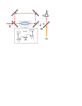
Figure 1: (color online) Schematic diagram of homodyne detection.

These discussions lend itself naturally to the final component of our model. To begin with, we note that $\hat{N}_{0}$ does not commute with $\hat{H}$ and cannot serve as a quantum nondemolition measurement (QND) variable Jacobs07 , and thus, the probe field is to remain as weak as the measurement permits in order to minimize its back-action on the signal. As the photons leaking from the cavity are combined with those from a strong local oscillator prior to the measurement by the photodetector, the homodyne detection scheme illustrated in Fig. 1 can greatly enhance the signal to noise ratio while at the same time allows us to directly measure the quadrature phase amplitude and hence the $\langle\hat{N}_{0}\rangle$-dependent probe phase shift as discussed above. In practice, in order to gain the spin dynamics, one must monitor the phase shift continually, and perform many runs of experiments, each of which provides a continual stream of information about $\langle\hat{N}_{0}\rangle$, before one can average over all the runs to construct the ensemble average $\langle\langle\hat{N}_{0}\rangle\rangle$. The stochastic master equation approach, which combines the system-reservoir theory with the photon counting theory Carmichael93 , is believed to be an excellent tool to simulate such experimental processes. This is the approach we take in the present study.

We begin with the measurement outcome, i.e., photodetector current $I$ (for a single run), which, after subtracting the constant part due solely to the coherent local oscillator, reads Wiseman93 ; Carmichael93

$$I=2\kappa\left\langle\hat{a}+\hat{a}^{\dagger}\right\rangle+\sqrt{2\kappa}\frac{dW\left(t\right)}{dt},$$ (3)

where $\kappa$ is the cavity decay rate, and $dW(t)/dt$ represents Gaussian white noise with $dW(t)$ an infinitesimal Wienner increment satisfying the Itô rules, $\langle\langle dW\left(t\right)\rangle\rangle=0$ and $dW\left(t\right)^{2}=dt$ Gardiner85 .

For the system subject to a continuous homodyne detection, its time evolution, conditioned on a given set of measurement outcomes, is described by the stochastic master equation (SME)

$$\frac{d\rho_{c}}{dt}=-\frac{i}{\hbar}[\hat{H},\rho_{c}]+2\kappa\mathcal{L[}\hat{a}]\rho_{c}+\sqrt{2\kappa}\frac{dW(t)}{dt}\mathcal{H[}\hat{a}]\rho_{c},$$ (4)

where $\rho_{c}$ is the conditional density matrix operator for the cavity mode + condensate system, and $\mathcal{L}$ and $\mathcal{H}$ are the superoperators defined as

$$\mathcal{L[}\hat{x}]\rho =\hat{x}\rho\hat{x}^{\dagger}-\frac{1}{2}\hat{x}^{\dagger}\hat{x}\rho-\frac{1}{2}\rho\hat{x}^{\dagger}\hat{x},$$

$$\mathcal{H[}\hat{x}]\rho =\hat{x}\rho+\rho\hat{x}^{\dagger}-\text{Tr}\left(\hat{x}\rho+\rho\hat{x}^{\dagger}\right)\rho.$$

The first term on the right-hand side of Eq. (4) represents the unitary evolution of the system under $\hat{H}$.  The second term describes the decay of the cavity, originating from coarse graining over the reservoir degrees of freedom. The last term is related to the quantum state collapse accompanied by the detection of each photoelectron at the detector; the fact that it shares with the current in Eq. (3) the same noise term, $dW(t)/dt$, indicates that the evolution of $\rho_{c}$ is indeed conditioned on the current measurement. Both the second and the last term can affect the dynamics of the cavity field and the spinor condensate.

To clearly show the measurement back-action on the spinor BEC, we consider that the measurement system operates in the regime where the cavity field decays at a rate much faster than the mean-field phase shift due both to the dispersive atom-photon coupling, and to the two-body s-wave scattering of atoms. Under such a condition, we can approximate $\hat{a}$ around a mean value $\alpha\equiv\left\langle\hat{a}\right\rangle\approx\eta/\kappa$ (the field amplitude of an empty cavity) with a small fluctuation $\hat{a}^{\prime}$according to $\hat{a}=\alpha+\hat{a}^{\prime}$, and eliminate the modes defined by the bosonic operator $\hat{a}^{\prime}$ adiabatically Gagen92 . In this way, we arrive at the dimensionless SME for the conditional density operator $\rho_{sc}=\mathrm{{Tr_{cavity}}\rho_{c}}$ of the spinor BEC alone

$$\frac{d\rho_{sc}}{d\tau}=-i[\hat{H}^{\prime},\rho_{sc}]+2\xi^{2}\mathcal{L[}\hat{N}_{0}]\rho_{sc}+\sqrt{2}\xi\frac{dW^{\prime}}{d\tau}\mathcal{H[}\hat{N}_{0}]\rho_{sc},$$ (5)

as well as the scaled photoelectric current

$$I^{\prime}=2\sqrt{2}\xi\langle\hat{N}_{0}\rangle+\frac{dW^{\prime}\left(\tau\right)}{d\tau},$$ (6)

where $\tau=\left|\lambda\right|t$ is the scaled time, $dW^{\prime}(\tau)/d\tau$ the scaled white noise, and $\xi=U_{0}\eta/\sqrt{\kappa^{3}\left|\lambda\right|}$ the measurement strength note1 . If we were to ignore the measurement back-action, the spinor BEC would undergo a unitary evolution under the scaled effective Hamiltonian $\hat{H}^{\prime}=[\hat{H}_{s}+\hbar U_{0}(\hat{N}-\hat{N}_{0})\left|\alpha\right|^{2}-\hbar\delta\left|\alpha\right|^{2}]/\hbar\left|\lambda\right|$.  In what follows, in order to highlight the essential physics, we fix the detuning to $\delta=U_{0}N$   so that $\hat{H}^{\prime}$ becomes

$$\hat{H}^{\prime}= \frac{\lambda}{\left|\lambda\right|}[(\hat{N}_{+}-\hat{N}_{-})^{2}+(2\hat{N}_{0}-1)(\hat{N}_{+}+\hat{N}_{-})$$

$$+2\hat{c}_{0}^{\dagger}\hat{c}_{0}^{\dagger}\hat{c}_{+}\hat{c}_{-}+2\hat{c}_{+}^{\dagger}\hat{c}_{-}^{\dagger}\hat{c}_{0}\hat{c}_{0}]-q^{\prime}\hat{N}_{0},$$ (7)

(after removing a constant term $\hbar q\hat{N}$) where $q^{\prime}=\left(q+U_{0}|\alpha|^{2}\right)/\left|\lambda\right|$ is defined as a new quadratic Zeeman shift.

The last two terms at the right-hand side of Eq. (5) represent the measurement back-action to the spinor condensate. The first of these is proportional to the double commutator [$\hat{N}_{0},[\hat{N}_{0},\rho_{sc}]]$, which represents a source of decoherence in the quantum dynamics. It tends to damp the off-diagonal elements of the density matrix under the basis of the measured observable $\hat{N}_{0}$. It represents one form of measurement back-action as it originates from the fact that any measurements on the cavity mode require the use of an output coupler to couple the cavity mode to the field modes outside the cavity. The last term in Eq. (5) can again be traced to the measurement induced state collapse in quantum mechanics, which is a stochastic process and hence depends on the white noise. The dynamics obtained directly from Eq. (5) is called the conditional dynamics, while that obtained after the ensemble average is called the deterministic dynamics. The last term of Eq. (5) therefore affects the conditional, but not the deterministic dynamics. Finally, in principle, there exists another type of measurement back-action - atom heating due to the fluctuation of the optical dipole force Stamper08 . However, since such a fluctuation is proportional to the gradient of the cavity field intensity, we anticipate the heating effect in a traveling-wave cavity to be much weaker than what was observed in a standing-wave cavity Stamper08 , and therefore we neglect it entirely in our work here.

III Spin-mixing dynamics under the continuous measurements

III.1 Two-Atom Case

In this section, we apply the formalism outlined in the previous section to a two-atom “toy” model, which, in principle, can be realized in optical lattices Bloch05 , to illustrate the influence of measurement backaction. Due to the conservation of atom number and magnetization, a spin-1 BEC with two atoms and zero magnetization is effectively a spin-1/2 system with two basis states $\left|1\right\rangle\equiv\left|0,2,0\right\rangle$ and $\left|2\right\rangle\equiv\left|1,0,1\right\rangle$, where $|N_{+},N_{0},N_{-}\rangle$ is a Fock state with $N_{i}$ number of atoms in spin-$i$ component.  In this basis, $\hat{H}^{\prime}$ (with $q^{\prime}=0$) has the following matrix representation

$$\hat{H}^{\prime}=\frac{\lambda}{\left|\lambda\right|}\left(\begin{array}[c]{cc}0&2\sqrt{2}\\ 2\sqrt{2}&-2\end{array}\right),$$ (8)

which has two eigenvalues, $E_{a}=2\lambda/\left|\lambda\right|$ and $E_{b}=-4\lambda/\left|\lambda\right|$, and two corresponding eigenstates $\left|a\right\rangle=\sqrt{2/3}\left|1\right\rangle+\sqrt{1/3}\left|2\right\rangle$ and $\left|b\right\rangle=-\sqrt{1/3}\left|1\right\rangle+\sqrt{2/3}\left|2\right\rangle$. Here, $\left|a\right\rangle$ is the ground state when $\lambda<0$ (ferromagnetic case) and $\left|b\right\rangle$ is the ground state when $\lambda>0$ $($antiferromagnetic case).

The dynamics of any atomic observable $\hat{A}$ in a particular realization can be constructed with the help of SME (5) starting from

$$\frac{d}{d\tau}\langle\hat{A}\rangle=\text{Tr}\left(\frac{d\rho_{sc}}{d\tau}\hat{A}\right).$$ (9)

For our case here, we find that the dynamical equations for the three Hermitian operators defined as

$$\hat{S}_{x} =\frac{1}{\sqrt{2}}(\hat{c}_{+}^{\dagger}\hat{c}_{-}^{\dagger}\hat{c}_{0}\hat{c}_{0}+\hat{c}_{0}^{\dagger}\hat{c}_{0}^{\dagger}\hat{c}_{+}\hat{c}_{-}),$$

$$\hat{S}_{y} =\frac{i}{\sqrt{2}}(\hat{c}_{+}^{\dagger}\hat{c}_{-}^{\dagger}\hat{c}_{0}\hat{c}_{0}-\hat{c}_{0}^{\dagger}\hat{c}_{0}^{\dagger}\hat{c}_{+}\hat{c}_{-}),$$ (10)

$$\hat{S}_{z} =\hat{N}_{0}-1,$$

are closed and can be cast into a matrix form

$$\frac{d}{d\tau}\left(\begin{array}[c]{c}\langle\hat{S}_{x}\rangle\\ \langle\hat{S}_{y}\rangle\\ \langle\hat{S}_{z}\rangle\end{array}\right) =\left(\begin{array}[c]{ccc}-4\xi^{2}&\mp 2&0\\ \pm 2&-4\xi^{2}&\mp 4\sqrt{2}\\ 0&\pm 4\sqrt{2}&0\end{array}\right)\left(\begin{array}[c]{c}\langle\hat{S}_{x}\rangle\\ \langle\hat{S}_{y}\rangle\\ \langle\hat{S}_{z}\rangle\end{array}\right)$$ (20)

$$-2\sqrt{2}\xi\frac{dW^{\prime}}{d\tau}\left(\begin{array}[c]{c}\langle\hat{S}_{x}\rangle\langle\hat{S}_{z}\rangle\\ \langle\hat{S}_{y}\rangle\langle\hat{S}_{z}\rangle\\ \langle\hat{S}_{z}\rangle^{2}-1\end{array}\right).$$ (24)

Here the upper (lower) signs are for the antiferromagnetic (ferromagnetic) case. The terms associated with the coefficient $-4\xi^{2}$ represent the dampings, typical of the dynamics of an open system, which destroy the coherence and leaves the system in a mixed state composed of eigenstates of measured observables. In the current section, we only consider the antiferromagnetic case ($\lambda>0)$ as it does not exhibit a qualitatively different dynamics from the ferromagnetic case.

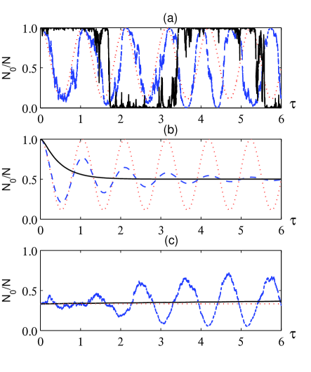
Figure 2: (color online) The evolution of the fractional population in spin-0: $N_{0}/N$. (a) and (b) show the conditional and deterministic evolution, respectively, with the initial state $\left|1\right\rangle$ and $q^{\prime}=0$. The red dotted line is for non-measurement case $\xi=0$, while the blue dashed line and black solid line is for weak measurement $(\xi=0.5)$ and strong measurement $(\xi=2)$ case, respectively. In (c), the initial state is $\left|b\right\rangle$ (see text) and $\xi=0.1$. The blue dashed line shows the conditional evolution while the black solid line shows the deterministic one. The red dotted line is for non-measurement case.

Consider two atoms that are initially prepared in state $\left|1\right\rangle$. Figures 2(a) and (b) illustrate, respectively, conditional and deterministic dynamics for systems with $\xi=0$ (red dotted lines), $0.5$ (blue dashed lines), and $2$ (black solid lines). For the case of no measurement ($\xi=0$), the population dynamics, $\langle\hat{N}_{0}\rangle/N=(1+\langle\hat{S}_{z}\rangle)/N$, undergoes a Rabi-type oscillation with frequency $|E_{a}-E_{b}|=6$. For a relatively weak measurement ($\xi=0.5$), besides some superimposed noises, the oscillation in a single run begins to experience a diffusive phase shift relative to the one without measurement; this results in a damped oscillation that one expects when many oscillations with different phase shifts are averaged. For a relatively strong measurement ($\xi=2$), the spin dynamics is drastically different. This is due to that the system is “watched” so frequently that Quantum Zeno effect (QZE) begins to manifest itself Milburn88 . Indeed, the conditional evolution indicates that repeated observations tend to trap the system in states $\left|1\right\rangle$ and $\left|2\right\rangle$, the only two states at which the noise term in Eq. ($\ref{bloch})$ vanishes. The extra time that the system spends either in $\left|1\right\rangle$ or $\left|2\right\rangle$ in the conditional evolution slows down the transition of the initial state to other states as shown in the deterministic evolution, which decays exponentially without any oscillations. In both weak and strong measurements, deterministic evolutions converge to a mixed state $(\langle\hat{S}_{x}\rangle=0,\langle\hat{S}_{y}\rangle=0,\langle\hat{S}_{z}\rangle=0)$, the only fixed-point of the deterministic part of Eqs. (24) at which the density matrix takes the diagonal form: $\rho_{sc}=0.5\left|1\right\rangle\left\langle 1\right|+0.5\left|2\right\rangle\left\langle 2\right|$.

Let us now discuss Fig. 2 (c), which displays the dynamics of two atoms initially prepared in the antiferromagnetic ground state $\left|b\right\rangle$. In the absence of any measurements, as expected, the system stays in its ground state (red dotted line). For a weak measurement ($\xi=0.1$), the system develops a Rabi-type oscillations in the conditional evolution, and is shown to attempt to converge to the mixed state in the deterministic evolution (black solid line). As before, QZE appears (not shown) when the measurement is sufficiently strong. In the two-atom case, a system starting from the antiferromagnetic ground state exhibits similar dynamics as that starting from the ferromagnetic ground state. However, in the $N$-atom case, as we show in the subsection below, due to the difference in the energy level structure and quantum fluctuation of $\hat{N}_{0}$, the measurement back-action will have quite distinct effects on the ferromagnetic and antiferromagnetic ground states.

III.2 $N$-Atom Case: Conditional Population Dynamics

Now we illustrate the measurement back-action effect for a condensate with $N=100$ atoms. We also adopt realistic parameters: $\kappa=2\pi\times 100$ MHz, $g_{0}=2\pi\times 1.6$ MHz, and $\lambda=2\pi\times 20$ Hz for sodium atoms with a typical density $10^{14}$ cm^-3 Lett09 .  We estimate that the value of $\xi$ lies in the range between $10^{-3}$ and $10^{-1}$ which means measurements here are always very weak. It is impossible to find a set of observables that are closed under Eq. (9) as in the two-atom case. However, under the assumption of perfect detection (with unit detection efficiency), we can unravel SME (5) into a equivalent stochastic Schrödinger equation (SSE) Carmichael93 in the sense $\rho_{sc}=\left|\psi_{sc}\right\rangle\left\langle\psi_{sc}\right|$ as

$$\frac{d}{d\tau}\left|\psi_{sc}\right\rangle =\left[-i\hat{H}^{\prime}-\xi^{2}(\hat{N}_{0}-\langle\hat{N}_{0}\rangle)^{2}\right.$$

$$\left.+\sqrt{2}\xi(\hat{N}_{0}-\langle\hat{N}_{0}\rangle)\frac{dW^{\prime}}{dt}\right]\left|\psi_{sc}\right\rangle,$$ (25)

which allows the dynamics of any observables to be calculated exactly. The simulation is performed using a fourth-order Runge-Kutta method for the deterministic part, and a first-order stochastic Runge-Kutta method for the noise part. Furthermore, the SSE (25) shows more clearly that the measurement back-action effects are dependent not only on the measurement strength, but also on the quantum fluctuation of the measured observable $\hat{N}_{0}$.

For the antiferromagnetic case, the ground state for $\hat{H}^{\prime}$ (with $q^{\prime}=0$) is unique and is given by a superposition of all the Fock states in which the spin-$1$ and $-1$ components share the same atom number:

$$\left|\psi\right\rangle=\sum_{k=0}^{[N/2]}A_{k}\left|k,N-2k,k\right\rangle,$$

where the amplitudes $A_{k}$ obey the recursion relation Law98

$$A_{k}=-\sqrt{\frac{N-2k+2}{N-2k+1}}A_{k-1}.$$

In this state, the average atom numbers in each spin component are equal, i.e., $\left\langle N_{+}\right\rangle=\left\langle N_{-}\right\rangle=\left\langle N_{0}\right\rangle=N/3$, and the number-fluctuation in spin-$0$ component is super-Poissonian for $N\gg 1$ Law98 . This indicates that the antiferromagnetic ground state will be quite sensitive to the measurement back-action effect.

Figure 3: Left column: Evolution of normalized particle number in spin-$0$ component under a single run of measurements with different strength (a) $\xi=0.001$, (b) $0.01$, and (c) $0.1$. The initial state is the anti-ferromagnetic ground state (see the text) with total atom number $N=100$. The corresponding Fourier spectra are shown in the right column.

Figures 3 illustrate the conditional population dynamics of atoms initially prepared in the antiferromagnetic ground state and the corresponding Fourier spectra for various measurement strengths. As Fig. 3(a) illustrates, a measurement as weak as $\xi=0.001$ can induce the system to oscillate predominantly at frequency $6\lambda$ (Fig. 3(d)), the first excited frequency of the many-body system described $\hat{H}^{\prime}$ in Eq. (7). As the measurement strength increases, more and more high-frequency components contribute to the evolutions. Fig. 3(b) is produced with $\xi=0.01$ which is ten times stronger than in Fig. 3(a). Indeed, instead of one peak, its Fourier spectrum [Fig. 3(e)] displays four peaks corresponding to the first fourth excited frequencies. Increasing $\xi$ by another factor of ten to $\xi=0.1$ leads to a more chaotic evolution as confirmed both by the population dynamics in Fig. 3(c) and by the corresponding Fourier spectrum in Fig.3 (f). Here, as a result of a dramatic increase in the number of eigenstates to which the system can collapse, QZE becomes more complicated. In Fig. 3(c), only the transitions to $\left|N/2,0,N/2\right\rangle$ and $\left|0,N,0\right\rangle$ are (dimly) visible because these two have the smallest transition moments to their neighboring eigenstates. In order to see QZE involving other transitions, we find from our numerical simulations that strong measurements with $\xi>10$ are typically needed.

Figure 4: Same as Fig. 3, except that for a ferromagnetic condensate. Insets show details of the oscillations.

The measurement back-action on ferromagnetic spinor condensates ($\lambda<0$) will take somewhat different effects because their distinct energy-level structures and quantum statistical properties. The ferromagnetic ground state is $2N+1$-fold degenerate, which reads Law98

$$\left|\psi_{m}\right\rangle=\sum_{k}B_{k}^{(m)}\left|k,N-2k-m,k+m\right\rangle,$$

where $m=0,\pm 1,\ldots,\pm N$. Contrary to the antiferromagnetic ground state, these states possess sub-Poissonian fluctuations in $\hat{N}_{0}$. To demonstrate the backaction, we choose the one with $m=0$ as the initial state, which has the largest fluctuation in $\hat{N}_{0}$.

In Fig. 4(a), the atomic population exhibits a weak Rabi-type oscillations with an amplitude much smaller than that for the antiferromagnetic case under the same measurement strength. The main reason for this reduction is, as indicated by the Fourier spectrum in Fig. 4(d), that the first excited frequency is located around $\omega=398$, which is much higher than that for the ferromagnetic case and hence is much difficult to excite. The reduction in the variance of $\hat{N}_{0}$ may also weaken the effect of measurement back-action. With the increase of the measurement strength, similar to the antiferromagnetic case, the spin populations oscillate with multiple frequencies and become irregular with some evidence of QZE, as shown in Figs. 4(b)-(f).

III.3 $N$-Atom Case: Comparison between Conditional and Deterministic Population Dynamics

The two examples considered in the previous subsection demonstrate the effect of the measurement back-action on the population dynamics of a single experimental realization, and as in the two-atom case, the deterministic dynamics will emerge from the average over many runs of numerical simulations. In order to make a smooth transition to the subject discussed in the next section, instead of pursuing such simulations with the two examples considered above, we seek to show the effect of averaging over many runs from a spinor BEC initially prepared in its mean-field ground state $\left|\psi\left(\tau=0\right)\right\rangle=\left|0,N,0\right\rangle$, where all the atoms reside in the spin-$0$ component.

Figure 5: (color online) (a) Time evolutions of $\langle\hat{N}_{0}\rangle/N$ for $q^{\prime}=10$ (upper curves) and $q^{\prime}=0$ (lower curves) case with the same initial state $\left|0,N,0\right\rangle$. The blue curves correspond to the evolution without measurement. The gray dotted curves display a variety of evolutions conditioned on measurement outcomes with measurement strength $\xi=0.01$, and the red curves are given by averaging over 10 conditional evolutions. (b) The number fluctuation of spin-0 component Var($\hat{N}_{0}$)=$\sqrt{\langle\hat{N}_{0}^{2}\rangle-\langle\hat{N}_{0}\rangle^{2}}$, with solid and dashed line corresponding to $q^{\prime}=10$ and $q^{\prime}=0$ case, respectively.

The spin-mixing dynamics, in the absence of the probe, can be well understood from the quantum-fluctuation-driven harmonic oscillator model FZhou08 . In Fig. 5(a), we compare the spin dynamics between $q^{\prime}=10$ (upper solid blue curve) and $q^{\prime}=0$ (low solid blue curve). In the former case, the oscillations are weak and approximately harmonic, while the latter case exhibits oscillations that are clearly of anharmonic nature. This is because quantum fluctuation in $\hat{N}_{0}$ is larger for small $q^{\prime}$ than for large $q^{\prime}$ as shown in Fig. 5(b). The spin dynamics for $q^{\prime}=0$ in a longer time scale is shown by the dashed blue curve in Fig. 6(a), which clearly demonstrates a typical quantum behavior - collapse and revival of spin oscillations. The particle number distribution quickly collapses to a metastable regime with $\langle\hat{N}_{+}\rangle=\langle\hat{N}_{-}\rangle=\langle\hat{N}_{0}\rangle/2=N/4$ after a time $\tau_{c}\simeq(2\sqrt{N})^{-1}$. This metastable regime is followed by several spin oscillations and the cycle repeats itself at a time interval $\tau_{r}=\pi$ Law98 .

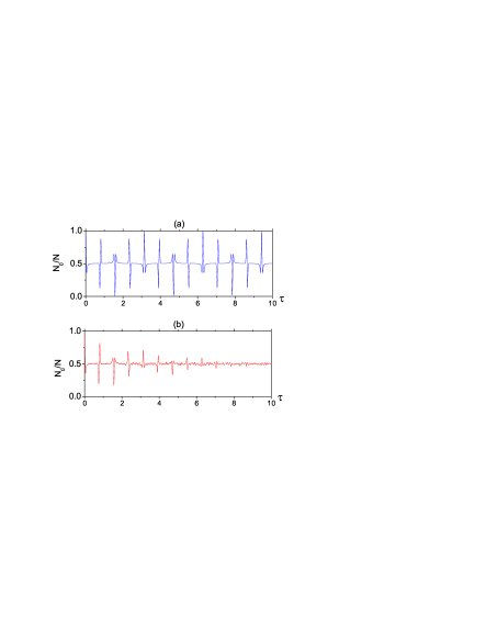
Figure 6: (color online) Comparing between the evolution without measurement (a) and the deterministic evolution (b) for the $q^{\prime}=0$ case in a long time scale.

In the presence of the probe, the spin-mixing dynamics will be affected by the measurement back-action. Various conditional evolutions with an intermediate measurement strength $\xi=0.01$ are plotted in gray dotted curves in Fig. 5(a). For the case $q^{\prime}=10$, they are not much different from the non-measurement evolution, so that averaging over 10 conditional evolutions appears sufficient to reveal the deterministic spin dynamics. The quantum measurement back-action are restrained by the small quantum fluctuation. In contrast, for the case $q^{\prime}=0$, they differ from the non-measurement evolution quite appreciably. In this case, averaging over 10 conditional evolutions (solid red curve) cannot produce the anticipated deterministic dynamics and the match is particularly poor in the metastable regime due to the large quantum fluctuation there. It requires more runs of measurements to reveal the deterministic spin evolution. The curve in Fig. 6(b) represents its deterministic evolution given by averaging over 100 conditional evolutions, which in a short time scale traces out the anharmonic spin oscillations clearly but indicates that the oscillations are gradually damped for a long time evolution. The damping rate is proportional to the measurement strength. Finally, the BEC converges to a mixed state characterized with a diagonal density matrix, $\rho_{sc}=\sum_{k=0}^{N/2}P_{k}\left|k,N-2k,k\right\rangle\left\langle k,N-2k,k\right|$, where the probability distribution function $P_{k}$ is found (not shown) to be a constant independent of $k$ or $P_{k}=1/(N/2+1)$ to be precise. All these are due to the decoherence induced by measurement as discussed in the two-atom case.

IV The Measurement Outcome: Photoelectric Current

The numerical simulations we have considered so far show that although each run results in a different conditional evolution $\langle\hat{N}_{0}\rangle$, an ensemble average over dozens of these runs can already capture quite well the deterministic quantum spin-mixing dynamics. However, what is accessible in experiments is not $\langle\hat{N}_{0}\rangle$ but the photoelectric current [Eq. (6)]. Thus, in practice, $\langle\langle\hat{N}_{0}\rangle\rangle$ must be inferred by averaging the current over many runs of measurements. As it turns out, it requires far more runs to reveal $\langle\langle\hat{N}_{0}\rangle\rangle$ indirectly from the ensemble average of the photoelectric current than directly from the ensemble average of conditional population dynamics.

Figures 7 (a) and (b) show the ensemble averages of the photodetector current $I^{\prime}$ for $N=10$ and $N=100$, respectively. The black curves represent the results given by $100$ runs of measurements. As can be seen, it is virtually impossible to extract the deterministic evolutions of $\langle\langle\hat{N}_{0}\rangle\rangle$ (shown in the insets) as they are dominated by white noise. In principle, one can suppress the noise by averaging over more and more currents; this is evident from the examples obtained when we increase the number of runs to 10³ (blue curve) and then to 10⁴ (red curve). However, only in $N=100$ case can the spin oscillations of deterministic nature be (vaguely) recognized. As for $N=10$ case, averaging the current over $10^{4}$ runs of measurements still do not allow us to extract the signal.

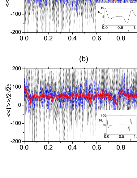
Figure 7: (color online) Measurement outcomes given by averaging over $10^{2}$ (black), $10^{3}$ (blue), and $10^{4}$ (red) photodetector currents. The total atom number $N$ is $10$ in (a) and $100$ in (b), and other parameters are the same as in Fig. 5. The insets show the deterministic evolution of $\langle\hat{N}_{0}\rangle$.

It appears that one could increase the measurement strength $\xi$ instead of the number of runs to enhance the signal to noise ratio according to Eq. (6). However, in quantum measurements, the system dynamics is conditioned on the detection outcomes; increasing the measurement strength also enhances the quantum measurement back-action. First, according to the discussion in Sec. II, strong measurement renders a large decoherence to the measured quantum state so that the spin oscillations is rapidly damped. Second, an increase in $\xi$ will increase the white noise in the stochastic Schrödinger equation, which in turn demands more runs to recover the deterministic dynamics. Thus, there is a limitation to what we can do to improve the signal to noise ratio by increasing the measurement strength.

An alternative is to increase the atom number. Not only does it enhance the signal part of the current in Eq. (6), but also it reduces the quantum fluctuation of $\hat{N}_{0}$ and thus the related measurement back-action. The net effect is the reduction in the number of required runs. But, as the atom number increases, the mean-field dynamics will gradually dominate Heinze10 , defeating the goal of extracting beyond-mean-field quantum dynamics from this measurement scheme. A possible way to increase the signal to noise ratio without raising the atom number is to process the current signal using methods such as filtering high frequency components and averaging over sliding windows Santamore04 . However, our study shows that more than $10^{3}$ runs are still needed before we can reveal the spin dynamics for a small BEC with less than $100$ atoms.

V Conclusion and Remarks

In this work, we have considered a homodyne detection scheme, which is designed to make a continuous measurement of the quantum spin-mixing dynamics of a small $F$=1 spinor BEC inside an optical cavity. Using the stochastic master equation approach, we have performed a detailed study of the quantum measurement back-action on the spin population dynamics in the bad cavity limit. We have used a simple two-atom system to illustrate both the measurement-induced quantum Zeno effect and the measurement-induced diffusive quantum dynamics. We have applied the physical intuitions gained from the two-atom model to understand the measurement back-action on the spin population dynamics in a spin-1 BEC. We have shown that the effect of back-action is sensitive to the quantum fluctuation of the spinor condensate. Finally, we stress that this study is motivated by recent proposals for using measurement techniques popular in cavity quantum optics to probe the quantum dynamics of small condensates. An important point we aim to make in this work is that when applying optical detection techniques to small condensates, one needs to pay close attention to quantum fluctuations, which are typically ignored for large condensates. Indeed, we have shown that due to the quantum measurement back-action, the number of runs of measurements, needed to recover the deterministic population dynamics from the ensemble average of the photoelectric current, increases as the number of atoms in the condensate decreases, suggesting that the scheme is not practical for sufficiently small condensates where the number of runs can become unrealistically large.

VI Acknowledgments

We thank JM Geremia for helpful discussions. This work is supported by the National Basic Research Program of China (973 Program) under Grant No. 2011CB921604, the National Natural Science Foundation of China under Grant No. 10588402 (W.Z.), No. 11004057 (L.Z.), and No. 10874045, the Program of Shanghai Subject Chief Scientist under Grant No. 08XD14017, Shanghai Leading Academic Discipline Project under Grant No. B480 (W.Z.), the “Chen Guang” project supported by Shanghai Municipal Education Commission and Shanghai Education Development Foundation (L.Z.) and the Fundamental Research Funds for the Central Universities (L.Z., K.Z.), and US National Science Foundation (H.P.,H.Y.L.), US Army Research Office (H.Y.L.), and Welch Foundation with Grant No. C-1669 (H.P.).

References

- (1) D. M. Stamper-Kurn, M. R. Andrews, A. P. Chikkatur, S. Inouye, H.-J. Miesner, J. Stenger, and W. Ketterle, Phys. Rev. Lett. 80, 2027 (1998); D. S. Hall, M. R. Matthews, J. R. Ensher, C. E. Wieman, and E. A. Cornell, Phys. Rev. Lett. 81, 1539 (1998).
- (2) T.-L. Ho, Phys. Rev. Lett. 81, 742 (1998); T. Ohmi and K. Machida, J. Phys. Soc. Jpn. 67, 1822 (1998); Weiping Zhang and D. F. Walls, Phys. Rev. A 57, 1248 (1998).
- (3) C. K. Law, H. Pu, and N. P. Bigelow, Phys. Rev. Lett 81, 5257 (1998).
- (4) J. Kronjäger, C. Becker, M. Brinkmann, R. Walser, P. Navez, K. Bongs, and K. Sengstock, Phys. Rev. A 72, 063619 (2005).
- (5) W. Zhang, D. L. Zhou, M.-S. Chang, M. S. Chapman, and L. You, Phys. Rev. A 72, 013602 (2005).
- (6) J. Heinze, F. Deuretzbacher, and D. Pfannkuche, Phys. Rev. A 82, 023617 (2010).
- (7) A. T. Black, E. Gomez, L. D. Turner, S. Jung, and P. D. Lett, Phys. Rev. Lett. 99, 070403 (2007).
- (8) M.-S. Chang, C. D. Hamley, M. D. Barrett, J. A. Sauer, K. M. Fortier, W. Zhang, L. You, and M. S. Chapman, Phys. Rev. Lett. 92, 140403 (2004); M. -S. Chang, Q. Qin, W. Zhang, L. You, and M. S. Chapman, Nature Physics 1, 111 (2005).
- (9) H. Schmaljohann, M. Erhard, J. Kronjäger, M. Kottke, S. van Staa, L. Cacciapuoti, J. J. Arlt, K. Bongs, and K. Sengstock, Phys. Rev. Lett. 92, 040402 (2004).
- (10) Y. Liu, S. Jung, S. E. Maxwell, L. D. Turner, E. Tiesinga, and P. D. Lett, Phys. Rev. Lett. 102, 125301 (2009).
- (11) J. Kronjäger, C. Becker, P. Navez, K. Bongs, and K. Sengstock, Phys. Rev. Lett. 97, 110404 (2006).
- (12) H. Pu and P. Meystre, Phys. Rev. Lett. 85, 3987 (2000); L.-M. Duan, A. Sørensen, J. I. Cirac, and P. Zoller, Phys. Rev. Lett. 85, 3991 (2000).
- (13) F. Brennecke, T. Donner, S. Ritter, T. Bourdel, M. Köhl, T. Esslinger, Nature (London) 450, 268 (2007).
- (14) J. M. Zhang, S. Cui, H. Jing, D. L. Zhou, and W. M. Liu, Phys. Rev. A 80, 043623 (2009).
- (15) X. Cui, Y. Wang, and F. Zhou, Phys. Rev. A 78, 050701(R) (2008).
- (16) L. Zhou, H. Pu, H. Y. Ling, and W. Zhang, Phys. Rev. Lett. 103, 160403 (2009); L. Zhou, H. Pu, H. Y. Ling, K. Zhang and W. Zhang, Phys. Rev. A 81, 063641 (2010).
- (17) Y. Dong, J. Ye, and H. Pu, Phys. Rev. A 83, 031608(R) (2011).
- (18) G. J. Milburn, J. Opt. Soc. Am. B 5, 1317 (1988); M. J. Gagen, H. M. Wiseman, and G. J. Milburn, Phys. Rev. A 48, 132 (1993).
- (19) M. J. Gagen and G. J. Milburn, Phys. Rev. A 45, 5228 (1992).
- (20) H. Pu, C. K. Law, S. Raghavan, J. H. Eberly, and N. P. Bigelow, Phys. Rev. A 60, 1463 (1999).
- (21) K. Jacobs, P. Lougovski, and M. Blencowe, Phys. Rev. Lett. 98, 147201 (2007).
- (22) H. J. Carmichael, An Open Systems Approach to Quantum Optics (Springer-Verlag, Berlin, 1993).
- (23) H. M. Wiseman and G. J. Milburn, Phys. Rev. A 47, 642 (1993).
- (24) C. W. Gardiner, Handbook of Stochastic Methods (Springer-Verlag, Berlin, 1985).
- (25) K. W. Murch, K. L. Moore, S. Gupta, and D. M. Stamper-Kurn, Nature Physics 4, 561 (2008).
- (26) We note that is negative in red-detuned case but we only give its absolute value in the following discussions.
- (27) A. Widera, F. Gerbier, S. Fölling, T. Gericke, O. Mandel, and I. Bloch, Phys. Rev. Lett. 95, 190405 (2005).
- (28) D. H. Santamore, A. C. Doherty, and M. C. Cross, Phys. Rev. B 70, 144301 (2004).