Buneman instability in a magnetized current-carrying plasma with velocity shear

Abstract

Buneman instability is often driven in magnetic reconnection. Understanding how velocity shear in the beams driving the Buneman instability affects the growth and saturation of waves is relevant to turbulence, heating, and diffusion in magnetic reconnection. Using a Mathieu-equation analysis for weak cosine velocity shear together with Vlasov simulations, the effects of shear on the kinetic Buneman instability are studied in a plasma consisting of strongly magnetized electrons and cold unmagnetized ions. In the linearly unstable phase, shear enhances the coupling between oblique waves and the sheared electron beam, resulting in a wider range of unstable eigenmodes with common lower growth rates. The wave couplings generate new features of the electric fields in space, which can persist into the nonlinear phase when electron holes form. Lower hybrid instabilities simultaneously occur at $k_{\shortparallel}/k_{\perp}\sim\sqrt{m_{e}/m_{i}}$ with a much lower growth rate, and are not affected by the velocity shear.

I Introduction

The Buneman instability has been extensively studied in theory and simulation since it was discovered in 1958 Buneman (1958). It is well-known in one-dimensional (1D) theory that once the relative drift of ions and electrons exceeds the threshold of approximately twice the electron thermal velocity, the interactions between waves and electrons will lead to the growth of the Buneman instabilityDavidson et al. (1970); Papadopoulos (1977). Lower hybrid instabilities lie on an oblique branch of current-driven instabilitiesMikhailovskii (1974); Kindel and Kennel (1971) with $k_{\shortparallel}/k\sim\sqrt{m_{e}/m_{i}}$. Their relation to Buneman instabilities has not been clarified yet in two-dimensional (2D) spectral space. Recently, interest in Buneman and lower hybrid instabilities has been renewed because of their importance in magnetic reconnectionDrake et al. (2003); Jovanović et al. (2005); Shokri and Niknam (2005); Fujimoto (2006); Dyrud and Oppenheim (2006); McMillan and Cairns (2007); Goldman et al. (2008); Che et al. (2009, 2010); Yoon and Umeda (2010). Magnetic reconnection is one of the most relevant mechanisms associated with explosive events in nature and in laboratory experiments, such as solar flares, substorms in the magnetosphere, and sawtooth crashes in fusion experiments.

Magnetic reconnection can convert magnetic field energy into thermal and kinetic energy. Oppositely directed magnetic fields merge and lead to the release of a significant fraction of the stored magnetic energy, which produces two regions of fast outflow (see Fig. 1). One of the most important problem in understanding magnetic reconnection is determining what mechanisms can facilitate reconnection fast enough to explain the explosive events observed. From magnetohydrodynamic (MHD) models, the convection and diffusion of the magnetic field can be described in terms of the magnetic Reynolds number $R_{m}=4\pi L_{0}V_{0}/c^{2}\eta^{2}$, where $L_{0}$ and $V_{0}$ are respectively the typical plasma velocity and magnetic field spatial length. If $R_{m}\ll 1$, the collisional resistivity can effectively dissipate the magnetic field’s energy and facilitate fast reconnection. However, the following question remains: What drives fast reconnection if the collision-induced resistivity is not sufficiently large (i.e. $R_{m}\gtrsim 1$)? This is a condition common in both space and laboratory plasmas. One of the most promising and physically interesting mechanism proposed to answer this question is turbulence-induced dissipation facilitating fast reconnectionSagdeev (1962); Davidson and Gladd (1975); Papadopoulos and Palmadesso (1976); Huba et al. (1977); Kulsrud (1998).

For turbulence-induced dissipation to work, the turbulence has to be generated spontaneously during the magnetic reconnection. In the diffusion region of magnetic reconnection, current sheets form as a result of changes in the magnetic field configuration. The intense thin current sheets which develop in strong guide field reconnection can drive streaming instabilities Drake et al. (2003); McMillan and Cairns (2007); Che et al. (2009, 2010) and electron velocity shear instabilitiesGanguli et al. (1988); Pritchett (1993); Drake et al. (1994); Nishimura et al. (2003); Ferraro and Rogers (2004); Che et al. etc. The latest 3D PIC simulations show that anomalous momentum transport generated by an electromagnetic electron velocity shear instability can influence the magnetic reconnection processChe et al. , but if turbulence resistivity can affect reconnection rates is still unclear. A deeper understanding of current-driven electrostatic instabilities is required. Buneman and lower hybrid instabilities are two of the most common electrostatic instabilities driven within current sheets in magnetic reconnection. They can produce electron holes and strong turbulent heating near the x-line and near the separatrix Farrell et al. (2002); Matsumoto et al. (2003); Ferraro and Rogers (2004); Vaivads et al. (2004); Cattell et al. (2005); Khotyaintsev et al. (2010); Che et al. (2010) (Fig.1).

Current sheets become thinner and thinner during reconnection, and velocity shear is generated in the current sheets regardless of the initial velocity distribution. Extensive studies on new instabilities driven by electron velocity shear within current sheets have been performedGanguli et al. (1988); Pritchett (1993); Drake et al. (1994); Ferraro and Rogers (2004); Eliasson et al. (2006). However, only a few studies have been carried out regarding how velocity shear affects the classical Buneman and lower hybrid instabilitiesReitzel and Morales (1998) although their role is important to the understanding of turbulence-induced dissipation processes in reconnection.

In this paper we investigate the role of weak velocity shear on Buneman and lower hybrid instabilities in 2D. Specifically, we study a plasma model consisting of strongly magnetized electrons and cold unmagnetized ions. A Mathieu equation analysis, first proposed by GoldmanGoldman et al. ; Goldman et al. (2005), is used and the results are compared with those of Vlasov simulationsNewman et al. (2007, 2008).The results we obtain from the Mathieu equation analysis are found to be consistent with the results from the Vlasov simulations with weak initial velocity shear, validating the approximations we adopted in the analytical method. We compare the Buneman instability driven by electrons with a uniform velocity drift (i.e., the classical Buneman instability) with the instability driven by drifting electrons with a weak cosine velocity shear. We find that the Buneman instability is no longer a purely magnetic field-aligned instability as commonly assumed in uniform beamBuneman (1958); Yoon and Lui (2008). The velocity shear enhances the interplay between oblique waves and electrons and produces a wide range of eigenmodes with a common growth rate lower than in the uniform-drift case. As shear increases, the fastest growing mode changes from a parallel plane wave to an eigenmode with significant oblique wavenumber content, as discussed in Appendix A. The shear does not significantly change the growth rate of the co-existing lower hybrid instability, which is much weaker than that of the Buneman instability under our assumptions. We obtain the eigenfunctions in 2D spectral space from the Mathieu equation analysis. These eigenfunctions show that the shear greatly modifies the 2D spatial structures of the instability-induced electric fields.

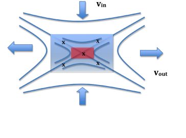
Figure 1: Illustration of magnetic reconnection. The red color indicates the electron diffusion region around the x-line with a scale of the electron skin depth $c/\omega_{pe}$. The semi-opaque blue color indicates the ion diffusion region with a scale of the ion skin depth $c/\omega_{pi}$. The inflow velocity is $v_{i}$ and the outflow velocity is $v_{o}$. The stars “*” mark some of the possible regions where electron holes can develop.

II Basic equations and solutions

II.1 Basic equations

We assume 1) the electrons are strongly magnetized such that $r_{e}=v_{te}/\Omega_{e}\ll\lambda_{e}=v_{te}/\omega_{pe}$, where $r_{e}$ is the electron cyclotron radius, $\lambda_{e}$ is the Debye length, $\omega_{pe}$ is electron plasma frequency, $v_{te}=\sqrt{\textit{k}T/m_{e}}$ is the electron thermal velocity, and k is Boltzmann’s constant. 2) the kinetic electrons are constrained to move along magnetic field lines while the ions are treated as unmagnetized and cold (i.e., the ratio of ion and electron temperature satisfies $T_{i}\ll T_{e}$). The validity of this assumption requires that the wave phase speeds are larger than ion thermal velocity.

We study the instabilities in the 2D $z$–$y$ plane. The electrons move along the $z$ direction with drift velocity $v_{b}(y)$. The magnetic field is treated as infinite in the $z$ direction for electrons and zero for ions, with no initial electric field ($E_{0}=0$). The initial ion drift velocity is also zero. The electron drift velocity is modulated by a weak cosine velocity shear:

$$v_{b}(y)=v_{0}[1+\varepsilon cos2\pi(y/L_{y}-0.5)],y\in[0,L_{y}],$$ (1)

where $\varepsilon$ is a small quantity and $L_{y}$ is the (spatial) periodicity of the shear profile.

Because the velocity shear is a function of $y$, the perturbed electric fields generated by instabilities are also functions of $y$. With the assumptions of cold ions and infinitely magnetized electrons, the perturbed and unperturbed functions do not depend on $v_{y}$. We perturb the Vlasov equation with $f_{q}=f_{0q}+\delta f_{q}=f_{0q}(v_{qz},y)+\delta f_{q}(v_{qz},y)e^{i(k_{z}z-\omega t)}$, where $q$ represents electrons ($e$) or ions ($i$). The electrostatic potential is $\delta\Phi=\phi(y)e^{i(k_{z}z-\omega t)}$. The cold ($|\omega/k|>v_{ti}$; here $v_{ti}$ is the ion thermal velocity) initial ion distribution function can be written as $f_{0i}=n_{0}\delta(v_{iy})\delta(v_{iz})$. To properly build our model, the initial electron distribution function is approximated by a 1D drifting kappa-functionSummers and Thorne (1991) with $\kappa=1$:

$$f_{0e}=\dfrac{2n_{0}}{\pi v_{te}}\left[1+\dfrac{(v_{ez}-v_{b}(y))^{2}}{v_{te}^{2}}\right]^{-2}.$$ (2)

The kappa-functions used to represent the electron distribution are quasi-Maxwellian at sub-thermal velocities, but with power-law rather than exponentially decreasing tails at supra-thermal velocities. Such power-law tails are a common feature of measured distributions in collisionless space plasmas. In our model the kappa distribution also simplifies the functional form of the susceptibilities, and thus enables us to obtain a specific mathematical differential equation with general solutions. We have compared our theoretical predictions to the results of 2D Vlasov simulations using both Maxwellian and kappa electron distributions, and find that the behavior in the two simulations is qualitatively equivalent. Only results from the simulations with Maxwellian electron distributions are presented in this paper.

After inserting the perturbations and initial conditions into the first order linear Vlasov equation and Poisson equation,

$$\frac{\partial\delta f_{q}}{\partial t} +v_{qz}\frac{\partial\delta f_{q}}{\partial z}-\frac{q}{m}\frac{\partial\delta\phi}{\partial z}\frac{\partial f_{0q}}{\partial v_{qz}}=0,$$ (3)

$$-\triangle\delta\Phi(y,k_{z},\omega)=4\pi(\rho_{e}+\rho_{i}),$$ (4)

we obtain

$$\frac{\partial^{2}\phi}{\partial y^{2}}-k_{z}^{2}(1+\frac{\chi_{ezz}}{1+\chi_{izz}})\phi=0,$$ (5)

$$\chi_{ezz}=-\dfrac{\omega_{pe}^{2}}{n_{0}k_{z}^{2}}\int_{C}\dfrac{\textsl{f}_{0e}(v_{ez})dv_{ez}}{(\frac{\omega}{k_{z}}-v_{ez})^{2}},$$ (6)

$$\chi_{izz}=-\dfrac{\omega_{pi}^{2}}{n_{0}k_{z}^{2}}\int_{C}\dfrac{\textsl{f}_{0i}(v_{iz})dv_{iz}}{(\frac{\omega}{k_{z}}-v_{iz})^{2}},$$ (7)

where $C$ indicates integration along the Landau contour in the complex plane, and $\rho_{e}$ and $\rho_{i}$ are the electron and ion charge density respectively.

Upon substituting $f_{0e}$ and $f_{0i}$ into (6) and (7) we find

$$\chi_{izz}=-\frac{\omega_{pi}^{2}}{\omega^{2}},$$ (8)

$$\chi_{ezz}=-\frac{\omega_{pe}^{2}}{k_{z}^{2}v_{tez}^{2}}\frac{\xi+3i}{(\xi+i)^{3}},$$ (9)

where $\xi=[\omega-k_{z}v_{b}(y)]/k_{z}v_{tez}$.

We normalize the quantities by defining $\omega\rightarrow\hat{\omega}\equiv\omega/\omega_{pe}$; $k_{z}\rightarrow K_{z}\equiv k_{z}v_{0}/\omega_{pe}$; $v_{tez}\rightarrow u_{e}\equiv v_{tez}/v_{0}$; $S\equiv(L_{y}\omega_{pe}/\pi v_{0})^{2}$, so that

$$\frac{\partial^{2}\phi}{\partial\theta^{2}}-SK_{z}^{2}(1+\frac{\chi_{ezz}}{1+\chi_{izz}})\phi=0,$$ (10)

$$\chi_{izz}=-\hat{\omega}_{pi}^{2}/\hat{\omega}^{2},$$ (11)

$$\chi_{ezz}=-\frac{1}{K_{z}^{2}u_{e}^{2}}\frac{\xi+3i}{(\xi+i)^{3}},$$ (12)

where $\theta\equiv\pi(y/L_{y}-0.5),\in[-\pi/2,\pi/2]$. For later use, we also define the normalization $k_{y}\rightarrow K_{y}\equiv k_{y}v_{0}/\omega_{pe}$.

Finally, we expand $\chi_{ezz}$ in $\varepsilon$ to the first-order and obtain

$$\frac{\partial^{2}\phi}{\partial\theta^{2}}+(a-2q\cos 2\theta)\phi=0,$$ (13)

where $\phi$ is a function of $\theta$, the parameters $a$ and $q$ are complex, and defined as

$$\eta=\frac{\hat{\omega}-K_{z}}{K_{z}u_{e}},\qquad a=-SK_{z}^{2}(1+\frac{\chi_{ezz0}}{1+\chi_{izz}})$$ (14)

and

$$q=-\frac{\varepsilon S}{u_{e}^{3}}\frac{\eta+4i}{(\eta+i)^{4}(1+\chi_{izz})},$$ (15)

so that

$$\chi_{ezz0}=\chi_{ezz}|_{\varepsilon=0}=-\frac{1}{K_{z}^{2}u_{e}^{2}}\frac{\eta+3i}{(\eta+i)^{3}}.\\$$ (16)

Equation (13) is the well-known Mathieu equation.

II.2 Solutions of the Mathieu Equation

The Mathieu equation (13) is written in standard formBogoliubov and Mitropolski (1961). The quantity $a$ is the characteristic value (or eigenvalue) and the parameter $q$ is defined in (15). For specific pairs $(a,q)$, the Mathieu equation has a unique analytical solution (eigenfunction) $\phi$, which can be written as $\phi_{r}(\theta)=e^{ir\theta}\tilde{\phi}_{r}(\theta)$, where $r$ is an integer or a rational number. The value $r$ is called the characteristic exponent, and $\tilde{\phi}_{r}$ is a complex function of $\theta$ that can be either even or odd. For periodic boundary conditions, $\phi_{r}$ has period $\pi$, and r is required to be integer. In the case of the electric field, $r$ is more restrictively required to be an even integer. If $q=0$, Eq. (13) reduces to the standard oscillator equation, where $r=\sqrt{a}$ and the solutions reduce to $\phi_{r}\propto\cos(\sqrt{a}\theta)$ (even function) and $\sin(\sqrt{a}\theta)$ (odd function).

The fact that $\phi_{r}=e^{ir\theta}\tilde{\phi}_{r}(\theta)$ suggests that the parameter $r$ is related to to the perpendicular wavenumber $k_{y}$. For the case $q=0$, a map $r=r(k_{y})$ can be established. In equation (13), $r$ is related to $\theta\equiv\pi(y/L_{y}-0.5)$ so that $\theta$ scales with the width of the box $L_{y}$; thus $k_{y}=r\pi/L_{y}$. However, for the case $q\neq 0$, the correspondence between $r$ and $k_{y}$ is nontrivial and needs an alternative treatment (see Appendix A).

We solve equation (13) with the given periodic boundary conditions in $r$–$K_{z}$ space for $\varepsilon=0$ and 0.2. The case of $\varepsilon=0$ implies $q=0$, which corresponds to uniform velocity drift. For specificity, we choose the following parameter values: $v_{0}=5v_{te}$, $L_{y}=256\lambda_{e}$, and the ratio of ion to electron mass is 1836, so that $S=266$. These parameters are the same as those used in the Vlasov simulations described in the next section. To allow comparison between the analytical solutions and our Vlasov simulations, we use the electric field eigenmodes $E_{z}^{eig}$ and $E_{y}^{eig}$ instead of $\Phi$:

$$\delta\Phi_{r} =\phi_{r}(\theta)e^{i(k_{z}z-\omega t)},$$ (17)

$$E_{z}^{eig} =-Re\left(\frac{\partial\delta\Phi_{r}}{\partial z}\right)=-Re\left(ik_{z}\phi_{r}(\theta)e^{i(k_{z}z-\omega t)}\right),$$ (18)

$$E_{\theta}^{eig} =-Re\left(\frac{\partial\delta\Phi_{r}}{\partial\theta}\right)=-Re\left(\frac{\partial\phi_{r}}{\partial\theta}e^{i(k_{z}z-\omega t)}\right),$$ (19)

$$E_{y}^{eig} =\frac{\pi}{L_{y}}E_{\theta}^{eig}.$$ (20)

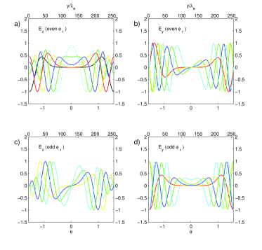
Figure 2: Eigenmodes of $E_{z}$ and $E_{y}$ for $z=0$ and $t=0$ calculated from both even and odd eigenfunctions of the electrostatic potential $\phi_{r}$ with even integer $r$ obtained from Mathieu equation (13). The lines colored black, red, yellow, green, blue, and cyan represent $r=$0, 2, 4, 6, 8, and 10, respectively. For odd eigenmodes, $r=2,4,6,8,10$.

For periodic boundary conditions we require not only that the eigenfunction $\phi$ be periodic, but also require that $E_{y}^{eig}$ be periodic so that the electric fields are continuous at the boundary. As we have mentioned only the eigenfunctions with even integer r can satisfy these continuity requirements. For odd eigenfunctions $\phi_{r}$ we require $r\neq 0$. For each value of $r$, the parallel wavenumber $K_{z}=k_{z}v_{0}/\omega_{pe}$ is chosen to maximize the eigenmode growth rate for that $r$. (See Fig. 3(b,c) below).

Figure 2 shows $E_{y}^{eig}$ and $E_{z}^{eig}$ at $z=0$ and $t=0$ for $\varepsilon=0.2$. For $E_{y}^{eig}$ and $E_{z}^{eig}$ obtained from even $\phi_{r}$, $r$=0, 2, 4, 6, 8, and 10; and from odd $\phi_{r}$, $r=2,4,6,8,10$. When $z=0$ and $t=0$, $E_{y}^{eig}\propto-\partial\phi_{r}/\partial y$ and $E_{z}^{eig}\propto\phi_{r}$. We scale $E_{z}^{eig}$ and $E_{y}^{eig}$ so that their maximum amplitudes are normalized to unity based on the assumption that all of the electric-field perturbations with different wavelength initially have approximately the same amplitude. For even $\phi_{r}$, we can see that $E_{y}^{eig}$ vanishes at $\theta=0$. By contrast, for even $\phi_{r}$, $E_{z}^{eig}$ vanishes at $\theta=0$ for small values of $r=0,2,4$ (black, red, and yellow lines, respectively) while $E_{z}^{eig}$ peaks for the larger values of $r$=8 and 10 (green and cyan lines, respectively). Comparing electric fields from odd $\phi_{r}$, $E_{y}^{eig}$ is similar to $E_{z}^{eig}$ from even $\phi_{r}$, but the peak value at $\theta=0$ of $E_{y}^{eig}$ (r=10) is much lower. $E_{z}^{eig}$ obtained from odd $\phi_{r}$ vanishes at $\theta=0$ for all $r$. These properties can produce specific features in the 2D electric fields that distinguish the electric fields in the sheared case from those produced by the instability driven by uniform electron drift. For $\varepsilon=0$, the initial electric-field eigenmodes at $z=0$ are proportional to either $\cos(r\theta)$ or $\sin(r\theta)$ with even integer $r$.

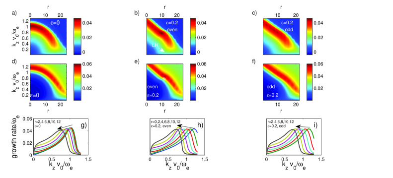
Figure 3: Theoretical growth rate in $r$–$K_{z}$ space in panel (a) and frequency in panel (d) for case $\varepsilon=0$; growth rate in panel (b) and frequency in panel (e) for even $\phi_{r}$ for $\varepsilon=0.2$ while growth rate in panel (c) and frequency in (f) are for odd $\phi_{r}$ for $\varepsilon=0.2$. respectively. The peak of the growth rate in (a) is around $(r,K_{z})\sim(0,1)$, the peak of the growth rate in (b) is around $(r,K_{z})\sim(10,0.8)$ and the peak of the growth rate in (c) is around $(r,K_{z})\sim(2,1.2)$. The symbol “+” in panels (e) indicate the position of the peak growth rate for $\varepsilon=0.2$ in $r$–$K_{z}$ space. Panels (g), (h) and (i) show 1D growth rates vs. $K_{z}$ for cases $\varepsilon=0$ and $\varepsilon=0.2$. The arrows in (g), (h) and (i) indicate the directions in which $r$ increases.

We obtained the linear frequency and growth rate of the unstable eigenmodes for both even and odd $\phi_{r}$ for each pair $(r,K_{z})$ for both $\varepsilon=0$ and $\varepsilon=0.2$. We show the results in Fig. 3. Panels (a), (b) and (c) show the growth rate (imaginary part of the frequencies) in $r$–$K_{z}$ space, and panels (d), (e) and (f) show the corresponding real wave frequencies. Panels (g), (h) and (i) are 1D growth rates vs. $K_{z}$ for some specific $r$ values for cases $\varepsilon=0$ and $\varepsilon=0.2$, respectively. The arrows in (g), (h) and (i) indicate the direction of increasing $r$.

The unstable eigenmodes for the uniform beam in panel (a) ($\varepsilon=0$) are concentrated in two distinct areas, representing two different instabilities, one strong and the other weak. The stronger instability is the parallel mode at $K_{y}\sim 0,K_{z}\sim 1$ with peak growth rate $\sim 0.05\omega_{pe}$, comparable to the cold plasma limit of the growth rate for the fast-growing mode of the Buneman instability $\gamma_{max}\sim\frac{\sqrt{3}\omega_{pe}}{2}(\frac{m_{e}}{2m_{i}})^{1/3}$, where $\omega_{pe}$ is the electron plasma frequency. The growth rate peaks around $K_{z}\sim 1$, the same as in the uniform cold plasma beam limit where $v_{0}=k_{z}/\omega_{pe}$, and the frequency is $\omega\sim 0.03\omega_{pe}$ [panel (d)], which is close to the cold-plasma limit $\omega_{r}\sim\frac{\omega_{pe}}{2}(\frac{m_{e}}{2m_{i}})^{1/3}$. The peak growth rate of the weaker lower-hybrid instability is located near $r=14$ and $K_{z}=0.03$, with a growth rate of $\sim 0.01$. Since $r=14$ corresponds to $K_{y}=k_{y}v_{0}/\omega_{pe}\sim 1$, we have $k_{z}/\sqrt{k_{z}^{2}+k_{y}^{2}}\sim k_{z}/k_{y}\sim 0.03\sim\sqrt{m_{e}/m_{i}}$, which corresponds to the ratio of the parallel to the perpendicular component of the wave vector of the lower hybrid instability. The corresponding frequency is $\sim 0.01\omega_{pe}\sim\omega_{pi}$ [panel (d)], also around the cold plasma limit for the lower hybrid instability $\omega_{lh}=\omega_{pi}/(1+\omega_{pe}^{2}/\Omega_{e}^{2})^{1/2}$, where $\omega_{pi}$ is the ion plasma frequency and $\Omega_{e}$ is the electron cyclotron frequency (effectively infinite in our model). The growth rate of the Buneman instability decreases steeply with $K_{z}$ when it passes the peak, but in panels (g), (h) and (i), we see that the 1D growth rate curves for $r=6,8,10,12$ exhibit a plateau at very small $K_{z}<0.1$ in all three cases; these plateaus are caused by the presence of the lower hybrid instability.

Lower hybrid waves are oblique and can interact with both ions and electrons. For the ordering $\Omega_{i}\ll\omega_{LH}\ll\Omega_{e}$, an approximation in which the electrons are treated as magnetized and the ions as unmagnetized is often justified. Under this approximation electrons resonate with waves through their motion parallel to the magnetic field, satisfying $\omega/k_{\parallel}\sim v_{d}$. At the same time, ions resonate with waves through their motion both parallel and perpendicular to the magnetic field satisfying $\omega/k\sim v_{i}$. The waves resonating with drifting electrons (in the ion rest frame) and ions can lead to the growth of both Buneman and lower hybrid instabilities, with the former dominated by ion motion parallel to $\mathbf{B}$ and the latter by ion motion perpendicular to $\mathbf{B}$. Oblique lower hybrid waves therefore transfer the parallel momentum of electrons predominantly to the perpendicular momentum of ions. Thus the lower hybrid instability can be thought as the oblique limit of the Buneman instability. In our model, electrons are assumed to be infinitely magnetized while ions are assumed to be unmagnetized and cold, which is the extreme limit of this model. The transfer of momentum does not increase the temperature of ions in our approximation.

When comparing Fig. 3(b,e) and (c,f) for the sheared beam $\varepsilon=0.2$, to Fig. 3(a,d) for uniform beam, it is obvious that the velocity shear has changed the location of the most unstable eigenmodes for even potential eigenfunctions $\phi_{r}$ [panel (b)] to $(r,K_{z})\approx(10,0.8)$, with a growth rate close to $0.05\omega_{pe}$. A number of eigenmodes with $r<14$ have a comparable growth rate. The corresponding frequency shown in panel (e) is $\sim 0.04\omega_{pe}$ (with the fastest-growing mode indicated by the white cross), which is slightly higher than without shear. The lower hybrid instability, however, is not affected by the velocity shear, which might be due to our assumption of cold ions. The unstable eigenmodes for odd potential eigenfunctions $\phi_{r}$ in panel (c) with $r<14$ have nearly equal growth-rate maxima, with that of the $r=2$ mode being slightly higher than for other unstable modes, but lower than the growth rate of the fastest-growing ($r=10$) eigenmode for even $\phi_{r}$. Thus we can conclude that the most unstable mode is still associated with the Buneman instability. The velocity shear enhances the coupling between oblique waves and electrons. The parallel phase speeds for both cases are around $0.03v_{0}$, matching the cold plasma limit.

III Results of Vlasov simulations and Comparisons with theory

We have carried out two 2D Vlasov simulations with two different velocity shears: $\varepsilon=0$ and $\varepsilon=0.2$. The simulation box size is $L_{y}\times L_{z}=256\lambda_{e}\times 800\lambda_{e}$. The velocity range is $[-15,15]v_{te}$. The grids in phase space are $(L_{z},v_{ez},v_{iz},L_{y},v_{ey},v_{iy})=(512,128,128,64,1,64)$. The time step is about $0.626\omega_{pe}^{-1}$ and The total simulation time is $\omega_{pe}t\sim 1004$. We initialize the simulations with Maxwellian distribution functions for both electrons and ions, and work in the initial ion rest frame. The electrons are given a mean drift $v_{0}=5v_{te}$ with a weak cosine velocity shear (for $\varepsilon\neq 0$) as shown in Eq. (1). The ion-electron mass ratio is $1836$. We assume that the magnetic field along $z$ is infinite for electrons, so the electron distribution function is restricted to a three-dimensional ($z$–$y$–$v_{z}$) phase space. The ions are assumed to be unmagnetized. The electron-ion temperature ratio is $5$ so that the ions are relatively cold.

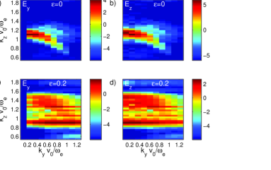
Figure 4: Panels (a) and (b) are, respectively, power spectra of $E_{y}$ and $E_{z}$ in logarithmic scale in 2D $k$ space at $\omega_{pe}t=552$ for the $\varepsilon=0$ Vlasov simulation; Panels (c) and (d) are the same as (a) and (b) for $\varepsilon=0.2$. [Note: some labels are cut off in the embedded PDF version of this figure.]

In §II.2 we have shown that both Buneman and lower hybrid instabilities can co-exist at the same time, but the lower hybrid instability is much weaker. Therefore in the Vlasov simulations we do not expect to observe the lower hybrid instability during the linear growth phase. In the case of $\varepsilon=0.2$, the fastest-growing unstable Buneman mode is the $r=10$ potential eigenmode for even $\phi_{r}$. This mode is dominant in the simulation while other unstable eigenmodes for $r=0,2,4,6,8$ for even $\phi_{r}$ compete with the unstable eigenmodes for odd $\phi_{r}$. To verify this we show the power spectra of the electric fields $|E_{y}(\mathbf{k})|^{2}$ and $|E_{z}(\mathbf{k})|^{2}$ in logarithmic scale at $\omega_{pe}t=552$ in both simulations in Fig. 4.

In the case of $\varepsilon=0$ [Fig. 4 (a, b)], the dominant $k$-space mode is parallel to $z$ (i.e., $k_{y}\approx 0$) with $K_{z}\sim 1.1$. A Fourier transform from the time domain over an interval containing $\omega_{pe}t=552$ reveals the frequency to be about $0.03\omega_{pe}$. Both the wavevector and frequency are consistent with the theoretical predictions for the Buneman instability with uniform electron velocity drift. The 2D power spectra $|E_{y}(\mathbf{k})|^{2}$ and $|E_{z}(\mathbf{k})|^{2}$ for $\varepsilon=0.2$ are shown in panels (c) and (d). We see that the strongest unstable modes for $E_{z}$ are now near $K_{z}=0.9$, which is consistent with the fastest-growing unstable $r=10$ eigenmode for even $\phi_{r}$ at $K_{z}\sim 0.8$ in Fig. 3b, and span a large range in $K_{y}$. The Fourier transform from the time domain shows the frequency increases slightly to $0.04\omega_{pe}$. In this case $r$ has a more indirect relation to $K_{y}$. Here we will use the mapping of eigenmodes from $r$ to $K_{y}$ discussed in Appendix A. For the globally fastest-growing eigenmode for even eigenfunctions $\phi_{r}$ at $r=10$ and $K_{z}=0.8$, the spectrum of $E_{z}(K_{y},K_{z})$ peaks near $K_{y}=0.2$. The neighboring $E_{z}$ even eigenmodes at $r=$4, 6, 8, and 12, which have almost as high a growth rate, exhibit multiple maxima in their $K_{y}$ spectra, with peaks both at low $K_{y}$ $(<0.2)$ and high $K_{y}$ $(>0.5)$ This behavior can be compared with that of corresponding synthetic $K_{z}$–$K_{y}$ spectra in Fig.9 and 10 of Appendix A. It is therefore reasonable to conjecture that the strongest modes of $E_{z}$ in Fig. 4 are produced by the higher-$r$ eigenmodes for even $\phi_{r}$ (e.g., $r=8$–12) for which $E_{z}^{eig}$ peaks near the center in Fig. 2a, although the width of the $E_{z}$ spectrum in $K_{z}$ from Fig. 4d is slightly narrower than would be expected based on the locus of growth-rate maxima (as a function of $r$) in Fig. 3b. The modes in Fig. 4 with $K_{z}\gtrsim 1.1$, by contrast, come from the low-$r$ eigenmodes for even $\phi_{r}$ (e.g., $r=0$–4), for which $E_{z}^{eig}$ peaks near the edge in Fig. 2a. The growth rate of unstable eigenmodes for odd $\phi_{r}$ compete with the lower $r$ eigenmodes for even $\phi_{r}$ and $K_{z}\sim 0.8$–$1.4$. These modes spread the spectrum of $E_{z}$. A similar argument can be used to explain the power spectrum of $E_{y}$. The $E_{z}$ and $E_{y}$ spectra for $\varepsilon=0.2$ peak at two distinct ranges of $K_{z}$, which come, respectively, from the two regions where $\partial v_{b}/\partial y$ vanishes: the center and edge of the box. At these locations $v_{b}$ is respectively 20% higher and 20% lower than for $\varepsilon=0$. Therefore, the dominant $K_{z}$ in each region should be $\sim$20% lower and $\sim$20% higher than for $\varepsilon=0$ if we apply the cold plasma relation $k_{z}=\omega_{r}/v_{b}$.

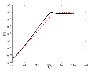
Figure 5: The growth in time of the spatially averaged electric field $\langle|E_{z}|\rangle$ in Vlasov simulations for $\varepsilon=$0 (black solid curve) and $\varepsilon=0.2$ (dashed red curve).

The time evolution of the spatially averaged electric fields in both simulations shown in Fig. 5 can be divided into two stages: linear and nonlinear. In the nonlinear stage the electric field reaches its peak and saturates via electron trapping. In the case of $\varepsilon=0.2$, electric fields become nonlinear slightly later than when $\varepsilon=0$ due to the small difference between the growth rates of the Buneman instability in these two cases. An effective growth rate $\gamma$ can be determined from the simulation fields during the linear phase through the relation $\gamma\Delta t\equiv\ln(E/E_{0})$. For $E\sim 1$ and $E_{0}\sim 10^{-13}$, $\omega_{pe}\Delta t=$600 and 700 corresponding to $\gamma\approx$ 0.05 and 0.043 for $\varepsilon=$0 and 0.2, respectively. These values are consistent with the results from linear kinetic theory shown in Fig. 3.

In Fig. 6, we show the electric fields $E_{z}$ and $E_{y}$ from Vlasov simulations in $z$–$y$ space. Panels (a) and (b) are for $\varepsilon=0$ at $\omega_{pe}t=679$ and panels (c) and (d) are for $\varepsilon=0.2$ at $\omega_{pe}t=753$, when the simulations for both cases are in a similar (late) nonlinear stage. These figures show localized and intense structures, indicative of electron trapping.

A comparison at a slightly earlier time of structures in $z$–$v_{z}$ phase space is shown in Fig. 7. Panel (a) is the electron distribution function $y=128\lambda_{e}$ for $\varepsilon=0$ at $\omega_{pe}t=627$, (b) is at $y=128\lambda_{e}$ and (c) is at the edge of $y$ for $\varepsilon=0.2$ at $\omega_{pe}t=691$. Again, because the instability with $\varepsilon=0$ grows faster than with $\varepsilon=0.2$, the evolution of electric fields and electron holes shown in Fig. 7 are both at approximately the same (early) nonlinear stage. That the width of electron holes in (c) is smaller than the width of electron holes in (b) is consistent with the wavelength of the Buneman instability in sheared beam. It’s interesting that the electron holes at the edge seems less regular than the electron holes at the center due to the fact that the electric field $E_{z}$ is weaker than the electric field $E_{z}$ at the center of $y$.

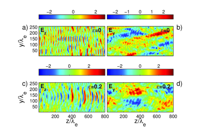
Figure 6: Panels (a) and (b) are the Vlasov-simulation electric fields $E_{z}$ and $E_{y}$ for $\varepsilon=0$ at $\omega_{pe}t=679$. Panels (c) and (d) are the same as (a) and (b) for $\epsilon=0.2$ and $\omega_{pe}t=753$. The two times correspond to approximately the same late nonlinear stage.

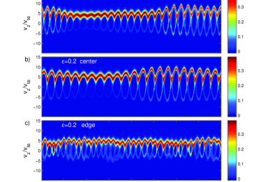
Figure 7: Panels (a), (b) and (c) are the Vlasov-simulation electron distribution functions in $z$–$v_{z}$ phase space. (a) is at $y=128\lambda_{e}$ for $\varepsilon=0$ at $\omega_{pe}t=$627; (b) is at the center and $y=128\lambda_{e}$ and (c) is at the edge of the $y$ for $\varepsilon=0.2$ at time $\omega_{pe}t=$691, respectively. The electron holes indicate that both simulations are at approximately the same early nonlinear stage.

To further demonstrate the eigenmode structure of the Buneman instability when $\varepsilon=0.2$, we compare 2D electric fields $E_{y}$, and $E_{z}$ based on the Mathieu-equation analysis to the electric fields in the linear stage of the corresponding Vlasov simulation at $\omega_{pe}t=552$. To do this, we construct a wavepacket of eigenfunctions with similar growth rates as a superposition of eigenfunctions with different weight and phase for $r=0$, 2, 4, 6, 8, 10, and 12 for even potential eigenfunctions $\phi_{r}$ and $r=2,4,6,8,10,12$ for odd potential eigenfunctions $\phi_{r}$. From the theoretical growth rate, we see that the features of the electric fields come mainly from the eigenmodes at $r=10$ for even potential eigenfunction $\phi_{r}$ and $r=2$ for odd potential eigenfunction $\phi_{r}$. The $r=10$ even eigenmode is dominated by small $K_{y}$ (long-wavelength) behavior near the center ($y=128\lambda_{e}$) while the $r=2$ odd eigenmode is dominated by large $K_{y}$ (short-wavelength) behavior near the edges. We draw the 2D $E_{z}$ structure synthesized from an eigenmode superposition in Fig. 8(a) and the corresponding $E_{y}$ in (b). Not surprisingly, we see that $E_{z}$ peaks at the center ($y/\lambda_{e}\sim 128$) where the drift is a maximum, while $E_{y}$ vanishes there. Compared to the electric fields at $\omega_{pe}t=552$ in the linear stage of the Vlasov simulation shown in Fig. 8 (c, d), the superposition of theoretical electric fields reproduces the main features of the simulation electric fields, but not necessarily all of the subtle details, which are controlled by the exact amplitudes and phases of the different contributing eigenmodes. We show the power spectra of the theoretical electric fields in 11 in Appendix. These features of the electric fields persist into the nonlinear stage, even after electron holes form (e.g., at $\omega_{pe}t\sim 700$, when the simulation has evolved into the nonlinear stage). Even though the electric fields shown in Fig. 6(c, d) become localized, we still see the $y$-dependence discussed above. On the other hand, $E_{z}$ in panel (a) and $E_{y}$ in panel (b) do not show any preferred value of $y$, as expected for a uniform (i.e., unsheared) electron beam.

Figure 8: Panels (a) and (b) show $E_{z}$ and $E_{y}$, respectively, in $z$–$y$ space as synthesized from a superposition of theoretically determined eigenmodes for $\varepsilon=0.2$; Panels (c) and (d) show $E_{z}$ and $E_{y}$, respectively, from the $\varepsilon=0.2$ Vlasov simulation at $\omega_{pe}t=552$, which is during the linear stage.

IV conclusion

In this paper we explored the impact of velocity shear on the Buneman and lower hybrid instabilities. We have studied the unstable modes for electron drifts modulated by a weak cosine velocity shear. In this case the dispersion relation can be approximated by the well-known Mathieu equation, where we used a kappa-function for the initial distribution of infinitely magnetized electrons (with cold unmagnetized ions), and we use a Taylor expansion for the velocity shear. These approximations have been validated by comparing the analytical results with the results of Vlasov simulations.

The effect of velocity shear is expected to strengthen the interactions between oblique waves and particles because shear causes the fastest-growing Buneman mode to change from a parallel plane wave to an eigenmode containing oblique as well as parallel Fourier modes. The shear also distributes the unstable Buneman eigenmodes over a wider range of eigenvalues, with nearly the same slightly lower growth rate than in the shear-free case. We conclude that the growth rate, wavelength, and orientation of the fastest growing Buneman mode are controlled by the presence (and amplitude) of shear in the electron velocity drift. Therefore, velocity shear can lead to different growth rates and wavelengths of unstable modes in the direction of the velocity gradient. The Vlasov simulation show that the electron holes form at both the center and the edge of the simulation box. At the center, electron trapping exhibits a longer wavelength consistent with the fact that the beam is at its fastest; at the edge, electron trapping exhibits a shorter wavelength, consistent with the correspondingly slower beam.

The velocity shear does not affect the growth rate of the weak lower hybrid instability, in which the interactions between lower hybrid waves and ions can transfer electron parallel momentum to the perpendicular motion of the ions. This momentum transfer can occur without necessarily affecting the temperature of the ions.

The advantage of our method is that it provides eigenfunctions for every unstable mode so that we can investigate both the spectra and 2D spatial structure of the electric fields. These results can help us to interpret the physical content of simulations, experiments and satellite data. Our method has assumed that the shear is weak. However, stronger velocity shear may reveal new physical regimes, including shear-driven as well as shear-modified instabilities. To address this issue, we are undertaking a study of how far the Mathieu-equation analysis can be extended.

Appendix A Mapping Mathieu equation eigenfunctions into Fourier space

We build a map between $r$ and $k_{y}$ by projecting the complex eigenmodes of $E_{y}(y,k_{z})$ and $E_{z}(y,k_{z})$ at t=0 into the $z$–$y$ plane,

$$E_{z}^{eig} = -Re(ik_{z}(\cos(k_{z}z)+i\sin(k_{z}z))(Re(\phi_{r})+iIm(\phi_{r})))$$ (21)

$$= k_{z}\cos(k_{z}z)Im(\phi_{r})+\sin(k_{z}z)Re(\phi_{r}),$$

$$E_{y}^{eig} = -\frac{\pi}{L_{y}}Re(ik_{z}(\cos(k_{z}z)+i\sin(k_{z}z))\frac{\partial}{\partial\theta}(Re(\phi_{r})+iIm(\phi_{r})))$$ (22)

$$= \frac{\pi}{L_{y}}(k_{z}\cos(k_{z}z)Im(\partial\phi_{r}/\partial\theta)+\sin(k_{z}z)Re(\partial\phi_{r}/\partial\theta)).$$

We then perform a 2D Fourier transformation of $E_{z}^{eig}$ and $E_{y}^{eig}$ in $(K_{y},K_{z})=v_{0}/\omega_{pe}(k_{y},k_{z})$ space. The results of Fourier transformation should be the same for even and odd eigenfunctions. In this appendix, we use even eigenfunctions $\phi_{r}$ to analyze the relation between $r$ and $K_{y}$. The results show that for $\varepsilon=0.2$ the corresponding power spectrum is no longer concentrated on one specific $K_{y}$ but is instead spread over a range of $K_{y}$, as shown in Fig. 9.

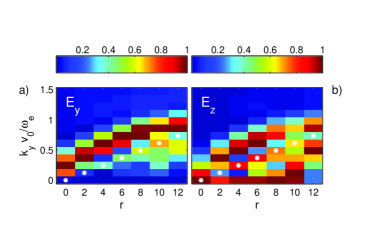
Figure 9: The correspondence between $K_{y}$ and even integer $r$. Panel (a) shows $E_{y}$ and panel (b) shows $E_{z}$ for $\varepsilon=0.2$. The white stars mark the linear correspondence $K_{y}=r\pi/L_{y}$ for $\varepsilon=0$.

We take the $K_{y}$ corresponding to the maximum power intensity. On the other hand the correspondence between $r$ and $K_{y}$ is different for $E_{y}$ and $E_{z}$. Fig 10 shows this map between $K_{y}$ and $r$. Black circle is for $E_{z}$. The $E_{z}$ eigenmodes $r=8,10,12$ have $K_{z}\sim 0.8$ while $r=10$ corresponds to $K_{y}\sim 0.2$, $r=6,8,12$ correspond to $K_{y}\sim 0.6,0,0.5$ respectively. $r=0$ eigenmode corresponds to $K_{y}\sim 0.1,K_{z}\sim 1.1$ and others in between $K_{z}\sim 0.8-1.1$ and $K_{y}\sim 0.1-0.6$. The $E_{y}$ eigenmodes for $r=0,2,4,6,8,10$ have a relatively linear correlation with $K_{y}$, but for $r=12$, $K_{y}$ decreases from $0.9$ to $0.5$.

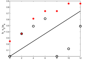
Figure 10: The correspondence between $K_{y}$ and $r$. The black circles are obtained for $E_{z}$ and red stars are for $E_{y}$ for the case $\varepsilon=0.2$. The black line is for $\varepsilon=0$.

To provide a fuller picture of the spectra from theory, we show in Fig. 11 the power spectra of the superposition of theoretical eigenmode electric fields $E_{y}$ and $E_{z}$ previously shown in Fig. 8.

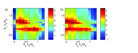
Figure 11: The power spectra for theoretical electric fields $E_{y}$ and $E_{z}$ shown in Fig. 8 (a, b). Panel (a) is for $E_{y}$ and panel (b) is for $E_{z}$.

We reiterate that the 2D theoretical $E_{y}$ and $E_{z}$ only reproduce the main features of the electric fields and thus the their power spectra shown in Fig. 11 can only approximate the realistic power spectra from the simulation as shown in Fig. 4. However, Figs. 4 and 11 do both show the same two distinct ranges of $K_{z}$. Again, the differences are controlled by the exact amplitudes and phases of the contributing eigenmodes, which we can not determine theoretically.

References

- Buneman (1958) O. Buneman, Phys. Rev. Lett. 1, 8 (1958)
- Davidson et al. (1970) R. C. Davidson, N. A. Krall, K. Papadopoulos, and R. Shanny, Phys. Rev. Lett. 24, 579 (1970)
- Papadopoulos (1977) K. Papadopoulos, Reviews of Geophysics and Space Physics 15, 113 (1977)NoStop
- Mikhailovskii (1974) A. B. Mikhailovskii, Theory of Plasma Instabilities, Vol. 1 (Consultants Bureau, New York, 1974)
- Kindel and Kennel (1971) J. M. Kindel and C. F. Kennel, J. Geophys. Res. 76, 3055 (1971)
- Drake et al. (2003) J. F. Drake, M. Swisdak, C. Cattell, M. A. Shay, B. N. Rogers, and A. Zeiler, Science 299, 873 (2003)
- Jovanović et al. (2005) D. Jovanović, P. K. Shukla, and G. Morfill, Phys. Plasma 12, 112903 (2005)
- Shokri and Niknam (2005) B. Shokri and A. R. Niknam, Phys. Plasma 12, 062110 (2005)
- Fujimoto (2006) K. Fujimoto, Phys. Plasma 13, 072904 (2006)
- Dyrud and Oppenheim (2006) L. P. Dyrud and M. M. Oppenheim, J. Geophys. Res. 111, 1302 (2006)
- McMillan and Cairns (2007) B. F. McMillan and I. H. Cairns, Phys. Plasma 14, 012103 (2007)
- Goldman et al. (2008) M. V. Goldman, D. L. Newman, and P. Pritchett, Geophys. Res. Lett. 35, 22109 (2008)
- Che et al. (2009) H. Che, J. F. Drake, M. Swisdak, and P. H. Yoon, Phys. Rev. Lett. 102, 145004 (2009), arXiv:0903.1311
- Che et al. (2010) H. Che, J. F. Drake, M. Swisdak, and P. H. Yoon, Geophys. Res. Lett. 37, 11105 (2010), arXiv:1001.3203
- Yoon and Umeda (2010) P. H. Yoon and T. Umeda, Phys. Plasma 17, 112317 (2010)
- Sagdeev (1962) R. Z. Sagdeev, in Electromagnetics and Fluid Dynamics of Gaseous Plasma (1962) pp. 443–+
- Davidson and Gladd (1975) R. C. Davidson and N. T. Gladd, Phys. Fluid 18, 1327 (1975)
- Papadopoulos and Palmadesso (1976) K. Papadopoulos and P. Palmadesso, Phys. Fluid 19, 605 (1976)
- Huba et al. (1977) J. D. Huba, N. T. Gladd, and K. Papadopoulos, Geophys. Res. Lett. 4, 125 (1977)
- Kulsrud (1998) R. M. Kulsrud, Phys. Plasma 5, 1599 (1998)
- Ganguli et al. (1988) G. Ganguli, Y. C. Lee, and P. J. Palmadesso, Phys. Fluid 31, 823 (1988)
- Pritchett (1993) P. L. Pritchett, Physics of Fluids B 5, 3770 (1993)NoStop
- Drake et al. (1994) J. F. Drake, R. G. Kleva, and M. E. Mandt, Physical Review Letters 73, 1251 (1994)
- Nishimura et al. (2003) K. Nishimura, S. P. Gary, H. Li, and S. A. Colgate, Phys. Plasma 10, 347 (2003)
- Ferraro and Rogers (2004) N. M. Ferraro and B. N. Rogers, Phys. Plasma 11, 4382 (2004)
- (26) H. Che, J. Drake, and M. Swisdak, Submitted to Nature
- Farrell et al. (2002) W. M. Farrell, M. D. Desch, M. L. Kaiser, and K. Goetz, Geophys. Res. Lett. 29, 190000 (2002)
- Matsumoto et al. (2003) H. Matsumoto, X. H. Deng, H. Kojima, and R. R. Anderson, Geophys. Res. Lett. 30, 060000 (2003)
- Vaivads et al. (2004) A. Vaivads, M. André, S. C. Buchert, J. Wahlund, A. N. Fazakerley, and N. Cornilleau-Wehrlin, Geophys. Res. Lett. 31, 3804 (2004)
- Cattell et al. (2005) C. Cattell, J. Dombeck, J. Wygant, J. F. Drake, M. Swisdak, M. L. Goldstein, W. Keith, A. Fazakerley, M. André, E. Lucek, and A. Balogh, J. Geophys. Res. 110, 1211 (2005)
- Khotyaintsev et al. (2010) Y. V. Khotyaintsev, A. Vaivads, M. André, M. Fujimoto, A. Retinò, and C. J. Owen, Physical Review Letters 105, 165002 (2010)
- Eliasson et al. (2006) B. Eliasson, P. K. Shukla, and J. O. Hall, Phys. Plasma 13, 024502 (2006)
- Reitzel and Morales (1998) K. J. Reitzel and G. J. Morales, Phys. Plasma 5, 3806 (1998)
- (34) M. V. Goldman, D. L. Newman, A. Mangeney, and F. Califano, 31st EPS Conf. Plasma Phys., 1.072 ECA 28G (2004)
- Goldman et al. (2005) M. Goldman, D. Newman, A. Mangeney, and F. Califano, Transport Theory and Statistical Physics 34, 225 (2005)
- Newman et al. (2007) D. L. Newman, N. Sen, and M. V. Goldman, Phys. Plasma 14, 055907 (2007)
- Newman et al. (2008) D. L. Newman, L. Andersson, M. V. Goldman, R. E. Ergun, and N. Sen, Phys. Plasma 15, 072902 (2008)
- Yoon and Lui (2008) P. H. Yoon and A. T. Y. Lui, Phys. Plasma 15, 112105 (2008)
- Summers and Thorne (1991) D. Summers and R. M. Thorne, Phys. Fluid B3, 1835 (1991)
- Bogoliubov and Mitropolski (1961) N. N. Bogoliubov and Y. A. Mitropolski, Asymptotic Methods in the Theory of Non-Linear Oscillations, by N. N. Bogoliubov and Y. A. Mitropolski. New York: Gordon and Breach, 1961., edited by Bogoliubov, N. N. & Mitropolski, Y. A. (1961)