Non-Markovian behavior of small and large complex quantum systems

Abstract

The channel induced by a complex system interacting strongly with a qubit is calculated exactly under the assumption of randomness of its eigenvectors. The resulting channel is represented as an isotropic time dependent oscillation of the Bloch ball, leading to non-Markovian behavior, even in the limit of infinite environments. Two contributions are identified: one due to the density of states and the other due to correlations in the spectrum. Prototype examples, one for chaotic and the other for regular dynamics are explored.

Introduction– Complex quantum systems are of paramount importance in the description of correlated many-body systems, such as the ones encountered in condensed matter, as well as few or single body chaotic systems. The exact description of such complex systems is often not possible because it is either unfeasible due to many degrees of freedom involved, or impossible because we do not know all the details of the microscopic model. Frequently we are also interested only in the dynamics of few degrees of freedom within a larger system. Unfortunately though, even in this case exact solutions are very rare. Under certain conditions, which are fulfilled in many important situations, one can use approximate methods. Such is the case if the central system of interest is only weakly coupled to the environment with fast decaying correlations. This leads to the description with a relatively simple Markovian Lindblad master equation Lindblad , implying a system without memory in which information flows only out from the central system. While specific models are known in which the reduced dynamics is not Markovian, general understanding is still lacking. Such questions resulted in a flurry of recent studies of non-Markovian behavior Jens ; Breuer ; Plenio ; other and characterization of reduced dynamics in general Wolf ; Chruscinski .

In the present work we shall derive an exact description of the reduced dynamics of a single qubit immersed in a complex system, undergoing unitary evolution. Our goal is to characterize the one-qubit channel induced by this unitary evolution. We shall assume that the eigenvectors of the Hamiltonian governing such evolution can be well described by a random unitary matrix. This is a very good approximation if the system is quantum chaotic Haake , but is also valid under more general circumstances.

Our main result can be expressed in a very simple geometrical picture. The derived one-qubit channel can be imagined as an isotropic shrinking of the Bloch ball. The radius of this Bloch ball however does not decrease monotonically with time but instead oscillates, causing non-Markovian behavior. The oscillations are due to (i) diffraction on the spectral density and, (ii) due to correlations between eigenenergy levels. Surprisingly, the first contribution will in general lead to non-Markovian behavior even for an infinite environment. Comparing the contribution due to eigenenergy correlations leads us to conclude that in the setting studied, chaotic systems display stronger non-Markovian behavior than regular ones, as quantified by measures proposed in Breuer ; Plenio . We also show, via exact expressions, that the channel is self-averaging for large sizes, meaning that non-Markovian behavior can be observed in individual system instances.

Setting– We study a system of dimension $N$, divided into a single qubit and the rest, acting as an environment to which the qubit is strongly coupled. The evolution of the total system is determined by a Hamiltonian $H$. The only requirement on $H$ is that the statistical properties of its eigenvectors are described by a random unitary matrix, which is connected to a maximum entropy principle balian . This is conjectured to happen for chaotic systems in the semiclassical limit, and is true, by construction, for the random matrix ensembles RMT suitable for describing statistical properties of quantum chaotic systems Haake . In quantum information language we want to characterize the quantum channel acting on the qubit. Once this is done we can study, for instance, whether the channel is markovian or not.

Assume that the initial state of the system is a factorizable state, with a projector in the environment. Other choices of initial states will be discussed later. The state at later times is thus simply

$$\rho_{\text{qubit}}^{(t)}=\mathop{\mathrm{tr}}\nolimits_{\text{env}}\left[U^{t}\rho_{\text{qubit}}^{(0)}\otimes|\psi_{\text{env}}\rangle\langle\psi_{\text{env}}|U^{-t}\right],$$ (1)

where $U^{t}=\exp{(-{\rm i}Ht)}$ (we set $\hbar=1$). This induces a completely positive map $\rho_{\text{qubit}}^{(t)}=\Lambda^{(t)}(\rho_{\text{qubit}}^{(0)})$. The matrix representation of this linear map in the basis of Pauli matrices is simply

$$\Lambda^{(t)}_{j,k}=\frac{1}{2}\mathop{\mathrm{tr}}\nolimits\left[\sigma^{j}\Lambda^{(t)}(\sigma^{k})\right],$$ (2)

where $i,j=0,\ldots,3$ with $\sigma^{j}=\{\sigma^{\rm x},\sigma^{\rm y},\sigma^{\rm z},\mathbbm{1}\}$.

Analytic derivation– We are interested in obtaining explicit expressions for eq. (2). Writing $H$ in its eigenbasis as $H=W\mathop{\mathrm{diag}}\nolimits(E_{i})W^{\dagger}$, where $W$ is the unitary matrix of eigenvectors of $H$, we are interested in properties of $\Lambda^{(t)}$ for a unitarily invariant ensemble of Hamiltonians where $W$ is a random unitary matrix. We shall calculate the average values of all matrix elements of channel $\Lambda^{(t)}$ as well as its fluctuations. One finds that given the invariance of $H$ under unitary rotations, the average channel, ie., after averaging over the unitarily invariant Haar measure of $W$, denoted by $\langle\cdot\rangle_{\mathcal{U}}$, must acquire a diagonal form in the Pauli basis (which can also be checked by an explicit calculation). Such channel is called depolarizing channel in quantum information. The matrix $\langle\Lambda^{(t)}_{j,k}\rangle_{\mathcal{U}}$ is therefore diagonal with time-dependent elements

$$\alpha(t):=\langle\Lambda^{(t)}_{0,0}\rangle_{\mathcal{U}}=\langle\Lambda^{(t)}_{1,1}\rangle_{\mathcal{U}}=\langle\Lambda^{(t)}_{2,2}\rangle_{\mathcal{U}}.$$ (3)

Trace preservation means that $\langle\Lambda^{(t)}_{3,3}\rangle_{\mathcal{U}}=1$ and $\langle\Lambda^{(t)}_{3,j=0,1,2}\rangle_{\mathcal{U}}=0$. All the physical information about the average channel, like the presence of non-Markovian effects, is contained in $\alpha(t)$, which is the radius of the evolved Bloch sphere of the qubit. The calculation of $\alpha(t)$ proceeds by separating the dependence of $U^{t}$ on the spectra $E_{i}$ and the eigenbasis $W$, $U^{t}=W\mathop{\mathrm{diag}}\nolimits\exp(-\mathrm{i}E_{i}t)W^{\dagger}$, to obtain

$$\alpha(t)=\mathrm{e}^{-\mathrm{i}(E_{i}-E_{j})t}\big{\langle}W_{0\mu,i}W_{00,i}^{*}W_{1\mu,j}^{*}W_{10,j}\\ +W_{0\mu,i}W_{10,i}^{*}W_{1\mu,j}^{*}W_{00,j}\big{\rangle}_{\mathcal{U}},$$ (4)

where we have used both Einstein’s summation convention and tensorial notation. Latin indices run over the whole system, whereas Greek ones run over the system minus the qubit. One can then average over the unitary Haar measure of $W$ using the exact formulas in Collins , obtaining the exact expression

$$\alpha(t)=\frac{N^{2}|f(t)|^{2}-1}{N^{2}-1},$$ (5)

with $f(t)=\frac{1}{N}\sum_{j}{\exp{(-{\rm i}E_{j}t)}}$ being the Fourier transform of the level density. The details of the calculation are to be found in the additional material Supplement .

The evaluation of the fluctuations of matrix elements is of interest, as it indicates how a single member of the ensemble will resemble the behavior of the ensemble average. Its calcultion involves 8-point correlations of $W$, and the Weingarten function for permutations on $4$ elements, which we have calculated Weingarten . Let us define by $\sigma^{2}_{j,k}=\langle[\Lambda^{(t)}_{j,k}]^{2}\rangle_{\mathcal{U}}-\langle\Lambda^{(t)}_{j,k}\rangle_{\mathcal{U}}^{2}$ the standard deviation of matrix element $\Lambda^{(t)}_{j,k}$. Again, due to the symmetry there are only three different fluctuations: those of diagonal matrix elements, those of off-diagonal elements in a $3\times 3$ block $\Lambda^{(t)}_{j,k}$ and those of $\Lambda^{(t)}_{i,3}$. The exact expressions to all orders in $1/N$ is given in the additional material Supplement , here we only give the leading terms in $1/N$, which are

$$\sigma^{2}_{i,i}=\sigma^{2}_{i,3} =\frac{1+(f^{*}(t)^{2}f(2t)+f(t)^{2}f^{*}(2t))-3|f(t)|^{4}}{2N},$$

$$\sigma^{2}_{i,j\neq i} =\frac{1+|f(t)|^{4}-(f^{*}(t)^{2}f(2t)+f(t)^{2}f^{*}(2t))}{2N},$$ (6)

with $i,j=0,1,2$. Equations (5) and (6) constitute our main result.

In the above results we have taken the initial state of the environment to be a projector. Due to the unitary invariance we can choose for $|\psi_{\text{env}}\rangle\langle\psi_{\text{env}}|$ any state. Because $\langle\Lambda^{(t)}_{j,k}\rangle_{\mathcal{U}}$ is linear in the initial state, any convex sum of projectors, ie., a density matrix of the environment, will also lead to the same average channel. Fluctuations though, which are not linear in the initial state, do change. In particular, the size of the fluctuations will scale as $\sim 1/(N\,r)$, if $r$ is the rank of the initial state of the environment. For instance, if the initial state of the environment is an identity matrix, corresponding to the environment at high temperature, the fluctuations scale as $\sim 1/N^{2}$ instead of $\sim 1/N$ as for the projector, meaning that self-averaging is stronger.

A random matrix example– We illustrate the above results by taking $H$ from the Gaussian Unitary Ensemble (GUE). This kind of Hamiltonians have been successfully used to describe a wide range of physical systems including chaotic systems, condensed matter systems and quantum environments RMT ; Haake ; pinedalong . For $t\to\infty$ the induced channel $\Lambda^{(t)}$ is closely related to the so-called random quantum channel, in which $U^{t}$ is replaced by a random unitary. Random quantum channels are usefull in quantum information theory Ion and have been used to prove that the conjecture about superaditivity of channel capacities is false aditivity . Because the joint probability distribution of eigenvalues is known for GUE we can perform explicit averaging over the spectrum, obtaining an expression for the average $f(t)$; note that due to self-averaging for large $N$ the average behavior is observed also in individual samples. As $\Lambda^{(t)}$ is quadratic in $f(t)$ it can be expressed in terms of 1- and 2-point correlations, which are known exactly for any dimension RMT . Strength of the interaction is fixed by $\langle|H_{i,j}|^{2}\rangle=\frac{1}{N}$, resulting in the spectral span of $4$ (determining the shortest time scale) and the Heisenberg time being $2N$ (giving the longest time scale, i.e., the inverse level spacing). The level density is $R_{1}(E)=\sum_{j=0}^{N-1}\varphi_{j}^{2}(E)$, where $\varphi_{j}(x)=\frac{{\rm e}^{-Nx^{2}/4}}{\sqrt{2^{j}j!\sqrt{2\pi/N}}}{\cal H}_{j}(x\sqrt{N/2})$ and ${\cal H}_{j}$ are Hermite polynomials. The cluster function, giving correlations between different levels, is for GUE $T_{2}(E_{1},E_{2})=\left(\sum_{j=0}^{N-1}\varphi_{j}(E_{1})\varphi_{j}(E_{2})\right)^{2}$. One can show that $N^{2}\langle|f(t)|^{2}\rangle_{\text{GUE}}=N+\int\mathrm{d}E_{1}\mathrm{d}E_{2}\mathrm{e}^{-\mathrm{i}(E_{1}-E_{2})t}[R_{1}(E_{1})R_{1}(E_{2})-T_{2}(E_{1},E_{2})]$, which can be evaluated explicitly for any $N$. Let us define $b_{2}(t)=(1/N)\int\mathrm{d}E_{1}\mathrm{d}E_{2}\mathrm{e}^{-\mathrm{i}(E_{1}-E_{2})t}T_{2}(E_{1},E_{2})$ and $b_{1}(t)=(1/N)\int\mathrm{d}E\mathrm{e}^{-\mathrm{i}Et}R_{1}(E)$. Normalization is such that $b_{1}(0)=1$ and $b_{2}(\infty)=0$. The final formula is

$$\langle\alpha(t)\rangle_{\rm GUE}=\frac{N^{2}b_{1}^{2}(t)+N(1-b_{2}(t))-1}{N^{2}-1}.$$ (7)

Each of the contributions approach a simple expression in the limit $N\to\infty$: $\lim_{N\to\infty}b_{1}(t)=\frac{J_{1}(2t)}{t}$, while the leading order of the form factor $1-b_{2}(t)$ is $t/2N$ for $t<2N$ and $1$ otherwise.

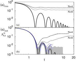
Figure 1: (a) Theoretical dependence of $\alpha(t)$ for Poisson example, Eq.(8) for $N=4,8$ and $\infty$. (b) Same three sizes for GUE example, Eq.(7). We also show three diagonal elements of $\Lambda^{(t)}$ for one instance of $N=12000$ (three thin blue curves) and theoretial fluctuations, displayed around $N=\infty$ theory as a gray shadow.

We can see that there are two contributions to $\langle\alpha(t)\rangle_{\rm GUE}$. The first one comes from the Fourier transformation of the energy density. The second one, given by the form factor and being due to eigenenergy correlations, is of the order $1/N$ compared to the first one, and is therefore important for moderate $N$. For large $N$ the second term can be neglected in Eq. 7, giving $\lim_{N\to\infty}\langle\alpha(t)\rangle_{\rm GUE}=[J_{1}(2t)/t]^{2}$. The form of $\langle\alpha(t)\rangle_{\rm GUE}$ for small and large $N$ in shown in Fig. 1b . There we also show fluctuations, which can be for large $N$ obtained by using $f(t)\approx J_{1}(2t)/t$ in Eq. 6 . The fluctuations decay with the system size as $\sim 1/N$. Therefore, for sufficiently large system the fluctuations are smaller than $\langle\alpha(t)\rangle_{\rm GUE}$, i.e., the dynamics is self-averaging. Even taking a single member $H$ of the GUE ensemble one gets the average behavior $\langle\alpha(t)\rangle_{\rm GUE}$, as can be seen in Fig. 1 for $N=12000$. If we would take the initial state of the environment to be the maximally mixed state, instead of $|\psi_{\text{env}}\rangle\langle\psi_{\text{env}}|$, similar self-averaging would be achieved already for $N\approx\sqrt{12000}\approx 100$, which is about $7$ qubits.

Poisson example– As a second example we show one still possessing unitary invariance, but having Poissonian eigenenergies with no correlations seligmanpoe , and with a flat level density, being a model for regular systems. The calculation goes exactly as in the previous example. Taking into account that there are no correlations among different levels and the spectral density is flat ($T_{2}(E_{1},E_{2})=0$, $R_{1}(E)=N\Theta\left(\left|E-2\right|\right)/4$, where $\Theta$ is the Heaviside step function), we get (see Fig. 1a)

$$\langle\alpha(t)\rangle_{\text{Poisson}}=\frac{N}{N+1}\left[\frac{\sin(2t)}{2t}\right]^{2}+\frac{1}{N+1}.$$ (8)

Non-Markovian behavior– Having calculated $\alpha(t)$, one can immediately draw conclusions about the non-Markovian behavior of the channels. Consider the map that takes a state from a time $t$ to $t+\tau$, $\Lambda^{(t,t+\tau)}=\Lambda^{(t+\tau)}\left[\Lambda^{(t)}\right]^{-1}$. This is, in general, not a physical map, which implies that the trace one operator associated via the Jamiołkowski isomorphism $\mathcal{J}$ is not a physical state. In Plenio , the deviation of positivity for such operators is taken as a measure of non-Markovian behavior $\mathcal{M}_{1}$. We define

$$g(t)\equiv\lim_{\epsilon\to 0^{+}}\frac{||\mathcal{J}(\Lambda^{(t+\epsilon,t)})||_{1}-1}{\epsilon}=\left\{\begin{array}[]{cl}\frac{3\dot{\alpha}(t)}{2\alpha(t)}&\mbox{ if $\dot{\alpha}(t)>0$}\\ 0&\mbox{ otherwise}\end{array}\right.$$ (9)

which will be positive whenever $\alpha(t)$ increases (the details are presented in the supplementary material Supplement ). With this figure of merit one can calculate the values of $\mathcal{M}_{1}=\int_{0}^{\infty}g(t)\mathrm{d}t$. A different criterion is based on the evolution of distinguishability of states with time Breuer and is defined as $\mathcal{M}_{2}=\max_{\rho_{0,1}(0)}\int_{\sigma>0}\mathrm{d}t\sigma(\rho_{0},\rho_{1},t)$, where $\sigma(\rho_{0}(t),\rho_{1}(t))$ is derivative of the trace distance between $\rho_{0,1}(t)$. The states $\rho_{0,1}$ that maximize such quantity for our channel are any two orthogonal pure states, say $\rho_{i}=|i\rangle\langle i|$. In such case $\rho_{i}(t)=\frac{\openone\pm\alpha(t)\sigma_{x}}{2}$ and $\mathcal{M}_{2}=2\int_{\dot{\alpha}>0}\mathrm{d}t\dot{\alpha}(t)$. The last measure to be examined quantifies non-Markovian behavior via the non-monotonicity of entanglement decay of our qubit with an ancilla qubit Plenio and is as such, as we will see, weaker than $M_{1,2}$: $\mathcal{M}_{3}=\int_{\dot{C}>0}\mathrm{d}t[\mathrm{d}C(\rho(t))/\mathrm{d}t]$, where $C$ is a measure of entanglement (to be taken here as the concurrence concurr ), $\rho(0)$ is a Bell state in the two qubits and the quantum channel acts on a single qubit. The concurrence for the corresponding state will be in our case $C(\rho(\alpha))=\max\{0,(3\alpha-1)/2\}$. The final result is $\mathcal{M}_{3}=\frac{3}{2}\int_{\dot{\alpha}>0,\alpha>1/3}\dot{\alpha}\mathrm{d}t$. In table 1 we report several values of all three measures for different environments. We can see that both $\mathcal{M}_{1,2}$ indicate non-Markovian behavior exactly at times when $\alpha(t)$ increases, in other words, when the Bloch ball expands. If we explicitly write $\mathcal{M}_{1}=3/2\sum{\ln{(\alpha(t_{f}))}-\ln{(\alpha(t_{i}))}}$ and $\mathcal{M}_{1}=2\sum{\alpha(t_{f})-\alpha(t_{i})}$, where both summations are over all intervals $[t_{i},t_{f}]$ on which $\alpha(t)$ increases, it is also easy to understand why the behavior of $\mathcal{M}_{1,2}$ is different with $N$. Because of the divergence of logarithm at $0$, the behavior of $\mathcal{M}_{1}$ is dominated by values of $\alpha(t_{i})$ which decrease with $N$, eventually becoming $0$ for $N\to\infty$, causing the increase of $\mathcal{M}_{1}$ with $N$. On the other hand $\mathcal{M}_{2}$ is dominated by terms $\alpha(t_{f})$ that decrease with $N$, see Fig. 1b . For Poisson example $\mathcal{M}_{2}$ increases due to a trivial $N/(N+1)$ prefactor. Looking back at our results and the two examples of a GUE and Poissonian ensemble, we can see that for small times non-Markovian behavior is due to diffraction on the spectral density. Provided the spectral span $\Xi$ is finite, there will always be oscillations in $\alpha(t)$ on the time-scale $1/\Xi$, causing non-Markovian behavior. How fast these oscillations decay with time depends on the singularity at the spectral edge – sharper features lead to slower decay of oscillations with time. In condensed matter systems singularities at spectral edges (van Hove singularities) are quite common. Surprisingly, non-Markovian behavior is present even for an infinite environment, where one would perhaps expect that there is no “back-flow of information” from the environment to the qubit. For smaller systems the term with the 2-point correlations also leads to non-Markovian effects. Indeed, for chaotic systems $1-b_{2}(t)$ increases with time, leading to an additional increase of $\alpha(t)$. This contribution occurs on the time-scale of the inverse level spacing. Interesting to note is, that comparing the GUE case, mimicking chaotic systems, with the Poissonian for regular dynamics, shown in Fig. 1 , one can conclude that non-Markovian effects are stronger in chaotic systems than in regular ones. This is yet-another example of a counter intuitive behavior of quantum chaotic system. Another is their stability, where quantum chaotic systems can be less sensitive to perturbations than regular ones fid .

	GUE			Poisson
	$\mathcal{M}_{1}$	$\mathcal{M}_{2}$	$\mathcal{M}_{3}$	$\mathcal{M}_{1}$	$\mathcal{M}_{2}$	$\mathcal{M}_{3}$
$N=4$	$4.375$	$0.378$	$0$	$0.555$	$0.156$	$0$
$N=8$	$6.102$	$0.236$	$0$	$1.064$	$0.173$	$0$
$N\to\infty$	$\infty$	$0.051$	$0$	$\infty$	$0.195$	$0$

Table 1: Different values of non-Markovian behavior for several environments. Notice how the two measures $\mathcal{M}_{1,2}$ have different tendency for the GUE case, and how $\mathcal{M}_{3}$ can not be used to detect non-Markovian behavior in our systems.

Conclusion– We analytically calculate a quantum channel describing the reduced dynamics of a single qubit within a larger system. Unitary evolution by unitarily invariant Hamiltonian leads to simple diagonal channel that can be visualized as an isotropically oscillating Bloch ball. The average value of the diagonal matrix element has two contributions: (i) one from the Fourier transformation of the energy density, and (ii) from correlations between eigenenergies. Provided there is some eigenenergy repulsion, as is the case in quantum chaotic systems, the second contribution will lead to semiclassically small non-Markovian behavior. This effect is stronger for more chaotic systems. The contribution due to energy density in general leads to non-Markovian effects even in the limit of an infinite environment. We also calculate channel fluctuations, showing that the dynamics is self-averaging for large systems. This means that non-Markovian effects should be observable already in small individual systems, making it an exciting experimental challenge. Acknowledgments– Support by the Program P1-0044, the Grant J1-2208 of the Slovenian Research Agency, and projects CONACyT 57334 and UNAM-PAPIIT IN117310 are acknowledged.

I Supplementary material

I.1 Fluctuations of $\Lambda_{j,k}^{(t)}$

After straightforward but tedious calculation, we obtained exact results for all three different fluctuations. They can all be expressed in terms of the Fourier transformation of the level density denoted by $f(t)$ and its powers,

$$f(t):=\frac{1}{N}\sum_{j}\exp{(-{\rm i}E_{j}t)}.$$ (10)

Exact expressions (to all orders in $1/N$) for fluctuations of matrix elements of $\Lambda^{(t)}$ are the following (in these expressions no averaging over eigenenergies is performed yet; therefore, any spectrum can be used):

$$\begin{split}\langle[\Lambda_{0,0}^{(t)}]^{2}\rangle_{\mathcal{U}}=\frac{1}{2N(1-\frac{1}{N^{2}})(1-\frac{9}{N^{2}})}&\left[(1-\frac{9}{N^{2}})+(2-\frac{3}{N}-\frac{6}{N^{2}})\left\{N|f(t)|^{4}+\frac{1}{N}|f(2t)|^{2}-\frac{4}{N}|f(t)|^{2}\right\}+\right.\\ &\left.+(1-\frac{4}{N})\left\{[f^{*}(t)]^{2}f(2t)+[f(t)]^{2}f^{*}(2t)\right\}\right].\end{split}$$ (11)

To get the fluctuation, one has to subtract from the previous expression $\langle\Lambda^{(t)}_{0,0}\rangle^{2}$ (here the averaging over both, unitary and eigenenergies, has to be performed before squaring). Other two fluctuations are

$$\sigma^{2}(\Lambda_{0,3}^{(t)})=\frac{(1-\frac{2}{N})}{2N(1-\frac{1}{N^{2}})(1-\frac{9}{N^{2}})}\left[(1-\frac{9}{N^{2}})-3|f(t)|^{4}-\frac{3}{N^{2}}|f(2t)|^{2}+\frac{12}{N^{2}}|f(t)|^{2}+\left\{[f^{*}(t)]^{2}f(2t)+[f(t)]^{2}f^{*}(2t)\right\}\right].$$ (12)

$$\begin{split}\sigma^{2}(\Lambda_{0,1}^{(t)})=\frac{1}{2N(1-\frac{1}{N^{2}})(1-\frac{9}{N^{2}})}&\left[(1-\frac{9}{N^{2}})+|f(t)|^{4}+\frac{1}{N^{2}}|f(2t)|^{2}-\frac{4}{N^{2}}|f(t)|^{2}-\right.\\ &\left.-(1-\frac{6}{N^{2}})\left\{[f^{*}(t)]^{2}f(2t)+[f(t)]^{2}f^{*}(2t)\right\}\right].\end{split}$$ (13)

Notice that one gets correlations up to 4th order, including those that mix $f(t)$ at different times, making the exact averaging over eigenenergies, for instance in terms of Hermite polynomials for GUE, very cumbersome. In the leading order with respect to $1/N$ one can, often, forget about correlations, and interchange averages of powers with the powers of averages. Thus, if $h_{t}:=\langle f(t)\rangle_{\rm spectrum}$, we obtain for the leading order

$$\sigma^{2}(\Lambda^{(t)}_{0,0}) = \frac{1+(h_{t}^{*2}h_{2t}+h_{t}^{2}h_{2t}^{*})-3|h_{t}|^{4}}{2N},$$

$$\sigma^{2}(\Lambda^{(t)}_{0,1}) = \frac{1+|h_{t}|^{4}-(h_{t}^{*2}h_{2t}+h_{t}^{2}h_{2t}^{*})}{2N},$$

$$\sigma^{2}(\Lambda^{(t)}_{0,3}) = \sigma^{2}(\Lambda^{(t)}_{0,0}).$$ (14)

This approximation is indeed valid in both examples examined in the main text for large dimensions. For GUE ensemble $h_{t}=J_{1}(2t)/t$, giving very simple expression for correlations. They are shown in Fig. 2 . In Fig. 3 we also show the values of 6 off-diagonal matrix elements $\Lambda^{(t)}_{j,k}$, $j\neq k=0,1,2$, for one GUE instance of dimension $N=12000$ (the same data as shown in the main text). Because the average values of these off-diagonal elements is zero (thick line at $0$ in the figure), they simply fluctuate around $0$ with the amplitude given by theoretical $\sigma_{0,1}$, Eq.(14), and shown as a gray shadow in the figure.

Figure 2: Scaled fluctuations of matrix elements of $\Lambda^{(t)}$ for a GUE ensemble and large sizes, where one can use $h_{t}$ for $f(t)$.

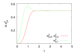
Figure 3: Values of off-diagonal elements of $\Lambda^{(t)}_{j,k}$, with $j\neq k=0,1,2$, for one GUE instance of size $N=12000$ (thin blue curves). Fluctuation $\sigma_{0,1}$ is shown as a gray shadow around the average at $0$ (thick red line).

For smaller size $N=4$, and again GUE ensemble, theoretical expressions for fluctuations (11,12,13) are shown in Fig. 4 . One can see that the time dependence is quite complicated.

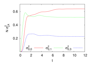
Figure 4: Theoretical formulas for fluctuations given in Eqs.(11,12,13) for size $N=4$. All is for a GUE ensemble.

General feature of fluctuations is that they are very small for short times, and reach their maximal value before the first revival in $\alpha(t)$ (this comes about due to the presence of $f(2t)$ term in fluctuations).

I.2 Details for the GUE calculation

We want to evaluate the quantity

$$\left\langle|f(t)|^{2}\right\rangle_{\text{GUE}}=\frac{1}{N^{2}}\left\langle\sum_{i,j}\mathrm{e}^{-\mathrm{i}(E_{i}-E_{j})t}\right\rangle_{\text{GUE}},$$ (15)

where averaging is over GUE spectrum. Such average can be written as

$$\left\langle\sum_{i,j}\mathrm{e}^{-\mathrm{i}(E_{i}-E_{j})t}\right\rangle_{\text{GUE}}=N+\\ \int\mathrm{d}E_{1}\mathrm{d}E_{2}\mathrm{e}^{-\mathrm{i}(E_{1}-E_{2})t}\left\langle\sum_{i\neq j}\delta(E_{1}-E_{i})\delta(E_{2}-E_{j})\right\rangle_{\text{GUE}}.$$ (16)

The quantity to be averaged is the two point correlation function:

$$R_{2}(E_{1},E_{2})=\left\langle\sum_{i\neq j}\delta(E_{1}-E_{i})\delta(E_{2}-E_{j})\right\rangle_{\text{GUE}},$$ (17)

which can be expressed in terms of the level density of states $R_{1}(E)$ and the two level cluster function $T_{2}(E_{1},E_{2})$:

$$R_{2}(E_{1},E_{2})=R_{1}(E_{1})R_{1}(E_{2})-T_{2}(E_{1},E_{2}),$$ (18)

for which explicit expressions in terms of Hermite polynomials exists. In particular,

$$R_{1}(E)=\sum_{j=0}^{N-1}\varphi^{2}_{j}(E),$$ (19)

and

$$T_{2}(E_{1},E_{2})=\left(\sum_{j=0}^{N-1}\varphi_{j}(E_{1})\varphi_{j}(E_{2})\right)^{2}.$$ (20)

with

$$\varphi_{j}(x)=\frac{{\rm e}^{-Nx^{2}/4}}{\sqrt{2^{j}j!\sqrt{2\pi/N}}}{\cal H}_{j}(x\sqrt{N/2}),$$ (21)

and ${\cal H}_{j}$ being the Hermite polynomials. Explicit expressions for moderate $N$s can be obtained by straightforward calculation with the aid of symbolic computational program. The final expression for the desired quantity is thus

$$\left\langle|f(t)|^{2}\right\rangle_{\text{GUE}}=\frac{N+\int\mathrm{d}E_{1}\mathrm{d}E_{2}\mathrm{e}^{-\mathrm{i}(E_{1}-E_{2})t}R_{2}(E_{1},E_{2})}{N^{2}},$$ (22)

where $R_{2}$, $R_{1}$ and $T_{2}$ are given in terms of the Hermite polynomials.

In the large $N$ limit, simple expressions are also available. The limit of the level density is known as the semicircle law, and yields an ellipse with semi axis determined by normalization. Its Fourier transform is a Bessel function $J_{1}$:

$$\int_{-\infty}^{\infty}\mathrm{d}ER_{1}(E)\mathrm{e}^{-\mathrm{i}Et}\xrightarrow{\ \text{large}N\ }N\frac{J_{1}(2t)}{t}.$$ (23)

For the second term, the integral in the large $N$ limit yields the well known two level form factor for the GUE:

$$\int\mathrm{d}E_{1}\mathrm{d}E_{2}\mathrm{e}^{-\mathrm{i}(E_{1}-E_{2})t}T_{2}(E_{1},E_{2})\\ \xrightarrow{\ \text{large}N\ }\left\{\begin{array}[]{rl}N-|t|/2&\mbox{ if $t<2N$}\\ 0&\mbox{ otherwise}\end{array}\right..$$ (24)

I.3 Measures of non-Markovian behavior

The depolarizing channel maps a state $\rho=\frac{\openone+\vec{r}\cdot\sigma}{2}\to\mathcal{D}_{\alpha}(\rho)=\frac{\openone+\alpha(t)\vec{r}\cdot\sigma}{2}$. This is precisely the map corresponding to $\langle\Lambda\rangle_{\mathcal{U}}$. We shall now work in the Choi basis, which is, for a single qubit, $\{|0\rangle\langle 0|,|0\rangle\langle 1|,|1\rangle\langle 0|,|1\rangle\langle 1|\}$. The matrix representation of such a channel, in the aforementioned basis is

$$\mathcal{D}_{\alpha}=\begin{pmatrix}\frac{1+\alpha}{2}&0&0&\frac{1-\alpha}{2}\\ 0&\alpha&0&0\\ 0&0&\alpha&0\\ \frac{1-\alpha}{2}&0&0&\frac{1+\alpha}{2}\end{pmatrix}.$$ (25)

One can also think of the map from a time $t_{1}$ to $t_{2}$, which is not necessarily physical. The matrix representation of such a map is

$$\mathcal{D}_{t_{2},t_{1}}=\begin{pmatrix}\frac{1}{2}+\alpha_{r}&0&0&\frac{1}{2}-\alpha_{r}\\ 0&\alpha_{r}&0&0\\ 0&0&\alpha_{r}&0\\ \frac{1}{2}-\alpha_{r}&0&0&\frac{1}{2}+\alpha_{r}\end{pmatrix}$$ (26)

with $\alpha_{r}=\alpha(t_{2})/\alpha(t_{1})$. The associated state, via the Jamiołkowski isomorphism $\mathcal{J}$ is

$$\mathcal{J}\mathcal{D}_{t_{2},t_{1}}=\frac{1}{2}\begin{pmatrix}\frac{1}{2}+\alpha_{r}&0&0&\alpha_{r}\\ 0&\frac{1}{2}-\alpha_{r}&0&0\\ 0&0&\frac{1}{2}-\alpha_{r}&0\\ \alpha_{r}&0&0&\frac{1}{2}+\alpha_{r}\end{pmatrix}$$ (27)

with eigenvalues $(1-\alpha_{r})/4$ (three times) and $(1+3\alpha_{r})/4$. With this one directly arrives to the result.

References

(1) V. Gorini et al., J. Math. Phys. 17, 821 (1976); G. Lindblad, Commun. Math. Phys. 48, 119 (1976).
(2) M. M. Wolf et al., Phys. Rev. Lett. 101, 150402 (2008).
(3) H.-P. Breuer et al., Phys. Rev. Lett. 103, 210401 (2009).
(4) Á. Rivas et al., Phys. Rev. Lett. 105, 050403 (2010).
(5) S. Daffer et al., Phys. Rev. A 70, 010304(R) (2004); S. Maniscalco and F. Petruccione, Phys. Rev. A 73, 012111 (2006); E.-M. Laine et al., Phys. Rev. A 81, 062115 (2010); L. Mazzola et al., Phys. Rev. A 81, 062120 (2010); B. Vacchini and H.-P. Breuer, Phys. Rev. A 81, 042103 (2010); T. J. G. Apollaro et al., Phys. Rev. A 83, 03
2103 (2011); D. Chruściński et al., Phys. Rev. A 83, 052128 (2011).
(6) M. M. Wolf and J. I. Cirac, Commun. Math. Phys. 279, 147 (2008).
(7) D. Chruściński and A. Kossakowski, Phys. Rev. Lett. 104, 070406 (2010).
(8) F. Haake, Quantum signatures of chaos, 3rd ed. (Springer, 2010).
(9) M. L. Mehta, Random matrices, 2nd ed. (Academic Press, New York, 1990); T. Guhr et al., Phys. Rep. 299, 189 (1998).
(10) B. Collins,
Int. Math. Res. Not. 17, 953 (2003).
(11) The Weingarten function is defined on the symmetric group of elements. The value depends only on the length of cycles in permutation (its cycle shape). For and it is given in Collins , for the values are , where and .
(12) Supplementary material.
(13) C. Pineda et al., New J. Phys. 9, 106 (2007).
(14) F.-M. Dittes et al., Phys. Lett. A 158, 14 (1991); M. Moshe et al., Phys. Rev. Lett. 73, 1497 (1994).
(15)R. Balian, Il Nuovo Cimento B 57, 183 (1968).
(16) B. Collins and I. Nechita, e-print arXiv:0910.1768.
(17) P. Hayden and A. Winter, Commun. Math. Phys. 284, 263, (2008); M. B. Hastings, Nature Physics 5, 255 (2009).
(18) S. Hill and W. K. Wooters, Phys. Rev. Lett. 78, 5022 (1997); W. K. Wooters, Phys. Rev. Lett. 80, 2245 (1998).
(19) T. Prosen and M. Žnidarič, J. Phys. A 34, L681 (2001); T. Prosen, Phys. Rev. E 65, 036208 (2002); T. Prosen and M. Žnidarič, J. Phys. A 35, 1455 (2002).