Pushing the limits for medical image reconstruction on recent standard multicore processors

Abstract

Volume reconstruction by backprojection is the computational bottleneck in many interventional clinical computed tomography (CT) applications. Today vendors in this field replace special purpose hardware accelerators by standard hardware like multicore chips and GPGPUs. Medical imaging algorithms are on the verge of employing High Performance Computing (HPC) technology, and are therefore an interesting new candidate for optimization. This paper presents low-level optimizations for the backprojection algorithm, guided by a thorough performance analysis on four generations of Intel multicore processors (Harpertown, Westmere, Westmere EX, and Sandy Bridge).

We choose the RabbitCT benchmark, a standardized testcase well supported in industry, to ensure transparent and comparable results. Our aim is to provide not only the fastest possible implementation but also compare to performance models and hardware counter data in order to fully understand the results. We separate the influence of algorithmic optimizations, parallelization, SIMD vectorization, and microarchitectural issues and pinpoint problems with current SIMD instruction set extensions on standard CPUs (SSE, AVX). The use of assembly language is mandatory for best performance. Finally we compare our results to the best GPGPU implementations available for this open competition benchmark.

1 Introduction and Related Work

1.1 Computed tomography

Computed tomography (CT) [1] is nowadays an established technology to non-invasively determine a three-dimensional (3D) structure from a series of 2D projections of an object. Beyond its classic application area of static analysis in clinical environments the use of CT has accelerated substantially in recent years, e.g., towards material science or time-resolved scans supporting interventional cardiology. The numerical volume reconstruction scheme is a key component of modern CT systems and is known to be very compute-intensive. Acceleration through special-purpose hardware such as FPGAs is a typical approach to meet the constraints of real-time processing. Integrating nonstandard hardware into commercial CT systems adds considerable costs both in terms of hardware and software development, as well as system complexity. From an economic view the use of standard x86 processors would thus be preferable. Driven by Moore’s law the compute capabilities of standard CPUs have now the potential to meet the requested CT time constraints.

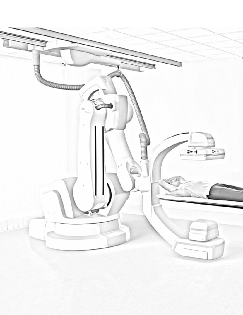
Figure 1: C-arm system illustration (Axiom Artis Zeego, Siemens Healthcare, Forchheim, Germany).

The volume reconstruction step for recent C-arm systems with flat panel detector can be considered as a prototype for modern clinical CT systems. Interventional C-arm CTs, such as the one sketched in Fig. 1, perform the rotational acquisition of 496 high resolution X-ray projection images (1248$\times$960 pixels) in 20 seconds [2]. This acquisition phase sets a constraint for the maximum reconstruction time to attain real-time reconstruction. In practice filtered backprojection (FBP) methods such as the Feldkamp algorithm [3] are widely used for performance reasons. The algorithm consists of 2D pre-processing steps, backprojection, and 3D post-processing. Volume data is reconstructed in the backprojection step, making it by far the most time consuming part [4]. It is characterized by high computational intensity, nontrivial data dependencies, and complex numerical evaluations but also offers an inherent embarrassingly parallel structure. In recent years hardware-specific optimization of the Feldkamp algorithm has focused on GPUs [5, 6] and IBM Cell processors [7]. For GPUs in particular, large performance gains compared to CPUs were reported [6] or documented by the standardized RabbitCT benchmark [8, 9]. Available studies with standard CPUs indicate that large servers are required to meet GPU performance [10]. In this report we also use the RabbitCT environment, which defines a clinically relevant test case and is supported by industry.

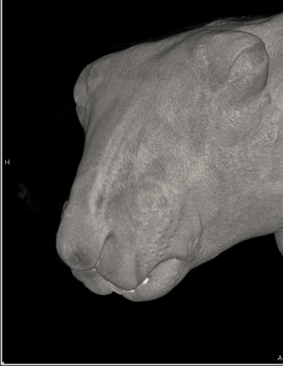
(a) Skin

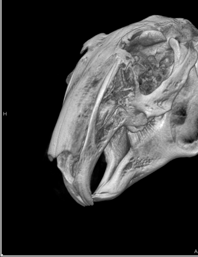
(b) Bones

Figure 2: Volume renderings based on the reconstruction of 2D X-ray projections of a rabbit.

RabbitCT is an open competition benchmark based on C-arm CT images of a rabbit (see Fig. 2). It allows to compare the manifold of existing hardware technologies and implementation alternatives for reconstruction scenarios by applying them to a fixed, well-defined problem.

At research level, recent reconstruction methods use more advanced iterative techniques, which can provide superior image quality in special cases like sparse or irregular data [11]. Other algorithms are used to reconstruct time-resolved volumes (“3D+$t$”) [12], e.g., for cardiac imaging. However, both approaches incorporate several backprojection steps, making performance improvements on the RabbitCT benchmark valuable for them as well. The same holds for industrial CTs in material science used in nondestructive testing (NDT), which additionally run at higher resolution and thus further increase the computational requirements [13]. The high computational demand of backprojection algorithms together with the growing acceptance of parallel computing in medical applications make them interesting new candidates on the interface to High Performance Computing.

1.2 Modern processors

The steadily growing transistor budget is still pushing forward the compute capabilities of commodity processors at rather constant price and clock speed. Improvement and scaling of established architectural features in the core (like, e.g., SIMD and SMT; see below for details) in addition to increasing the number of cores per chip lead to peak performance levels which enable standard CPUs to meet the time constraints of interventional CT systems. Optimized single core implementations are thus mandatory for reconstruction algorithms. Complemented by standard optimization techniques, a highly efficient SIMD (Single Instruction Multiple Data) code is the key performance component. Owing to the nontrivial data parallelism in the reconstruction scheme, SIMD optimizations need to be done at low level, i.e., down to assembly language. However, these efforts will pay off for future computer architectures since an efficient SIMD implementation will become of major importance to further benefit from increasing peak performance numbers.

Scaling SIMD width is a safe bet to increase raw core performance and optimize energy efficiency (i.e., maximize the flop/Watt ratio), which is known to be the critical component in future HPC systems. Recently Intel has played the game by doubling the SIMD width from the SSE instruction set (128-bit registers) to AVX [14] (256-bit registers, with larger widths planned for future designs), which is implemented in the “Sandy Bridge” architecture. More ongoing projects are pointing in the same direction, like Intel’s Many Integrated Core (MIC) [15] architecture or the Chinese Godson-3B chip [16]. Wider SIMD units do not change core complexity substantially since the optimal instruction throughput does not depend on the SIMD width. However, the benefit in the application strongly depends on the level and the structure of data parallelism as well as the capability of the compiler to detect and exploit it. Compilers are very effective for simple code patterns like streaming kernels [17], while more complex loop structures require manual intervention, at least to the level of compiler intrinsics. This is the only safe way to utilize SIMD capabilities to their full potential. The impact of wider SIMD units on programming style is still unclear since this trend currently starts to accelerate. Of course wide SIMD execution is most efficient for in-cache codes because of the large “DRAM gap.”

Simultaneous Multi-Threading (SMT) is another technology to improve core utilization at low architectural impact and energy costs. It is obvious that SMT should be most beneficial for those “in cache codes” that have limited single thread efficiency due to bubbles in arithmetic/logic pipelines, and where cache bandwidth is not the dominating factor. Naively one would not expect improvements from SMT if a code is fully SIMD-vectorized since SIMD is typically applied to simple data-parallel structures, which are a paradigm for efficient pipeline use. Since many programmers do not care about pipeline occupancy in their application the benefit of SMT is often tested in an experimental way, without arriving at a clear explanation for why it does or does not improve performance.

This paper is organized as follows. In Sect. 3 we perform a first analysis of the backprojection algorithm implemented in the RabbitCT framework using simple metrics like arithmetic throughput and memory bandwidth as guidelines for estimating performance. We address processors from four generations of Intel’s x86 family (Harpertown, Westmere, Westmere EX, and Sandy Bridge). Basic optimization rules such as minimizing overall work are applied. In Sect. 4 we show how to efficiently vectorize the inner loop kernel using SSE and AVX instructions, and discuss the possible benefit of multithreading with SMT. Sect. 5 provides an in-depth performance analysis, which will show that simple bandwidth or arithmetic throughput models are inadequate to estimate the performance of the algorithm. OpenMP parallelization and related optimizations like ccNUMA placement and bandwidth reductions are discussed in Sect. 6. Performance results for cores, sockets, and nodes on all four platforms are given in Sect. 7, where we also interpret the effect of the different optimizations discussed earlier and validate our performance model. Finally we compare our results with current GPGPU implementations in Sect. 8.

2 Experimental testbed

A selection of modern Intel x86-based multicore processors (see Table 1) has been chosen to test the performance potential of our optimizations. All of these chips feature a large outer level cache, which is shared by two (Core 2 Quad “Harpertown”), four (Sandy Bridge), six (Westmere EP), or ten cores (Westmere EX). We refer to the maximum number of cores sharing an outer level L2/L3 cache as an “L2/L3 group.”

With the initiation of the Core i7 architecture the memory subsystem of Intel processors was redesigned to allow for a substantial increase in memory bandwidth, at the price of introducing ccNUMA on multisocket servers. At the same time Intel also relaunched simultaneous multithreading (SMT, a.k.a. “Hyper-Threading”) with two SMT threads per physical core. The most recent processor, Sandy Bridge, is equipped with a new instruction scheduler, supports the new AVX SIMD instruction set extension, and has a new last level cache subsystem (which was already present in Nehalem EX). The 10-core Intel Westmere EX is not mainly targeted at HPC clusters but at large mission-critical servers. It reflects the performance maximum for x86 shared-memory nodes. A comprehensive summary of the most important processor features is presented in Table 1. Note that the Sandy Bridge model used here is a desktop variant, while the other processors are of the server (“Xeon”) type. Table 1 also contains bandwidth measurements for a simple update benchmark:

⬇

for(int i=0; i<N; ++i)

a[i] = s * a[i];

This benchmark reflects the data streaming properties of the reconstruction algorithm and is thus better suited than STREAM [17] as a baseline for a quantitative performance model.

We use the Intel C/C++ compiler in version 12.0; since most of our performance-critical code is written in assembly language, this choice is marginal, however. Thread affinity, hardware performance monitoring, and low-level benchmarking was implemented via the LIKWID tool suite [18, 19], using the tools likwid-pin, likwid-perfctr, and likwid-bench, respectively.

Table 1: Test machine specifications. The cacheline size is 64 bytes for all processors and cache levels. The update benchmark results were obtained with the likwid-bench tool.

Microarchitecture	Intel Harpertown	Intel Westmere	Intel Westmere EX	Intel Sandy Bridge
Model	Xeon X5482	Xeon X5670	Xeon E7- 4870	Core i7-2600
Label	HPT	WEM	WEX	SNB
Clock [GHz]	3.2	2.66 (2.93 turbo)	2.40	3.4 (3.5 turbo)
Node sockets/cores/threads	2/8/-	2/12/24	4/40/80	1/4/8
Socket L1/L2/L3 cache	4$\times$32k/2$\times$6M/-	6$\times$32k/6$\times$256k/12M	8$\times$32k/8$\times$256k/30M	4$\times$32k/4$\times$256k/8M
Bandwidths [GB/s]:
Theoretical socket BW	12.8	32.0	34.2	21.3
Update (1 thread)	5.9	15.2	8.3	16.5
Update (socket)	6.2	20.3	24.6	17.3
Update (node)	8.4	39.1	98.7	-

3 The algorithm

3.1 Code analysis

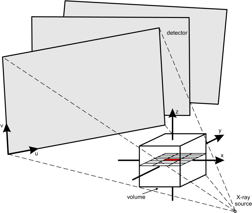
Figure 3: Setup geometry for generating the CT projection images. The size of the volume is always $256^{3}$ mm³, but the number of voxels may vary.

Listing 1: Voxel update loop nest for the plain backprojection algorithm. This gets executed for each projection I. All variables are of type float unless indicated otherwise. The division into parts (see text) is only approximate since there is no 1:1 correspondence to the SIMD-vectorized code.

⬇

1wz = offset_z;

2for(int z=0; z<L; z++, wz+=MM) {

3 wy = offset_y;

4

5 for (int y=0; y<L; y++, wy+=MM) {

6 wx = offset_x;

7 valtl=0.0f; valtr=0.0f;

8 valbl=0.0f; valbr=0.0f;

9

10 // Part 1 --------------------------

11 for (int x=0; x<L; x++, wx+=MM) {

12 uw = (A[0]*wx+A[3]*wy+A[6]*wz+A[9]);

13 vw = (A[1]*wx+A[4]*wy+A[7]*wz+A[10]);

14 w = (A[2]*wx+A[5]*wy+A[8]*wz+A[11]);

15

16 u = uw * 1.0f/w; v = vw * 1.0f/w;

17

18 int iu = (int)u, iv = (int)v;

19

20 scalx = u - (float) iu;

21 scaly = v - (float) iv;

22 // Part 2 ---------------------------

23 if (iv>=0 && iv<ISY) {

24 if (iu>=0 && iu<ISX)

25 valtl = I[iv*ISX + iu];

26 if (iu>=-1 && iu<ISX-1)

27 valtr = I[iv*ISX + iu+1];

28 }

29

30 if (iv>=-1 && iv<ISY-1) {

31 if (iu>=0 && iu<ISX)

32 valbl = I[(iv+1)*ISX + iu];

33 if (iu>=-1 && iu<ISX-1)

34 valbr = I[(iv+1)*ISX + iu+1];

35 }

36 // Part 3 ---------------------------

37 vall = scaly*valbl + (1.0f-scaly)*valtl;

38 valr = scaly*valbr + (1.0f-scaly)*valtr;

39 fx = scalx*valr + (1.0f-scalx)*vall;

40

41 VOL[z*L*L + y*L + x] += 1.0f/(w*w)*fx;

42 } // x

43 } // y

44} // z

The backprojection algorithm (as provided by the RabbitCT framework [9], see Listing 1) is usually implemented in single precision (SP) and exhibits a streaming access pattern for most of its data traffic. One volume reconstruction uses 496 CT images (denoted by I) of 1248$\times$960 pixels each (ISX$\times$ISY). The volume size is $256^{3}$ mm³. MM is the voxel size and changes depending on the number of voxels. The most common resolution in present clinical applications is 512 voxels in each direction (denoted by the problem size L). Each CT image is accompanied by a $3\times{}4$ projection matrix A, which projects an arbitrary point in 3D space onto the CT image. The algorithm computes the contributions to each voxel across all projection images. The reconstructed volume is stored in array VOL. Voxel coordinates (indices) are denoted by x, y, and z, while pixel coordinates are called u and v. See Fig. 3 for the geometric setup.

The aggregated size of all projection images is $\approx$$2.4$ GB. The total data transfer volume of one voxel sweep comprises the loads from the projection image and an update operation (VOL[i]+=s, see line 41 in Listing 1) to the voxel array. The latter incurs 8 bytes of traffic per voxel and results (for problem size $512^{3}$) in a data volume of $1$ GB, or $496$ GB for all projections. The traffic caused by the projection images is not easy to quantify since it is not a simple stream; it is defined by a “beam” of locations slowly moving over the projection pixels as the voxel update loop nest progresses. It exhibits some temporal locality since neighboring voxels are projected on proximate pixels of the image, but there may also be multiple streams with large strides. On the computational side, the basic version of this algorithm performs 13 additions, 5 subtractions, 17 multiplications, and 3 divides.

3.2 Simple performance models

Based on this knowledge about data transfers and arithmetic operations we can derive a first rough estimate of expected upper performance bounds. The arithmetic limitation results in 21 cycles per vectorized update (4 and 8 inner loop iterations for SSE and AVX, respectively), assuming full vectorization and a throughput of one divide per cycle. This takes into account that all architectures under consideration can execute one addition and one multiplication per cycle, neglects the slight imbalance of additions versus multiplications, and assumes that the pipelined rcpps instruction can be employed for the divisions (see Sect. 4.1 for details).

On the other hand, runtime can also be estimated based on the data transfer volume and the maximum data transfer capabilities of the nodes measured with the synthetic update benchmark described in Sect. 2. The following table shows upper performance bounds for a full $512^{3}$ reconstruction based on arithmetic and bandwidth limitations on the four systems in the testbed (full nodes):

	HPT	WEM	WEX	SNB
Arithm. lim. [GUP/s]	4.86	6.75	13.9	5.31
BW lim. [GUP/s]	1.06	4.90	11.1	2.15

Performance is given in billions of voxel updates per second (GUP/s), where one “update” represents the reconstruction step of one voxel using a single image. The low arithmetic limitation for the single socket Sandy Bridge is caused by its wide AVX vector size and its faster clock. While above predictions seem to indicate a strongly memory-bound situation, they are far from accurate: The runtime is governed by the number of instructions and the cycles it takes to execute these instructions. A reduction to the purely “useful” work, i.e., to arithmetic operations, can not be made since this algorithm is nontrivial to vectorize due to the scattered load of the projection image; it therefore involves many more non-arithmetic instructions (see Sect. 4.1 for details). We will show later that a more careful analysis leads to a completely different picture, and that further optimizations can change the bottleneck analysis considerably.

In order to have a better view on low-level optimizations we divide the algorithm into three parts:

1. Geometry computation: Calculate the index of the projection of a voxel in pixel coordinates

2. Load four corner pixel values from the projection image

3. Interpolate linearly for the update of the voxel data

3.3 Algorithmic optimizations

The first optimizations for a given algorithm must be on a hardware-independent level. Beyond elementary measures like moving invariant computations out of the inner loop body and reducing the divides to one reciprocal (thereby reducing the flop count to 31), a main optimization is to minimize the workload. Voxels located at the corners and edges of the volume are not visible on every projection, and can thus be “clipped off” and skipped in the inner loop. This is not a new idea, but the approach presented here improves the work reduction from 24% [21] to nearly 39%.

The basic building block for all further steps is the update of a consecutive line of voxels in $x$ direction, covered by the inner loop level in Listing 1. We refer to this as the “line update kernel.” The geometry, i.e., the position of the first and the last relevant voxel for each projection image and line of voxels is precomputed. This information is specific for a given geometric setup, so it can be stored and used later during the backprojection loop. Reading the data from memory incurs an additional transfer volume of $512^{2}$$\times$$496$$\times$$4$ bytes$=$$496$ MB/s (assuming 16-bit indexing), which is negligible compared to the other traffic. The advantage of line-wise clipping is that the shape of the clipped voxel volume is much more accurately tracked than with the blocking approach described in [21].

The conditionals (lines 23 and 30 in Listing 1), which ensure correct access to the projection image, involve no measurable overhead for the scalar case due to the hardware branch prediction. However, for vectorized code they are potentially costly since an appropriate mask must be constructed whenever there is the possibility that a SIMD vector instruction accesses data outside the projection [21]. To remove this complication, separate buffers are used to hold suitably zero-padded copies of the projection images, so that there is no need for vector masks. The additional overhead is far outweighed by the performance advantage for vectorized code execution. The conditionals are also effectively removed by the clipping optimization described above, but we need a code version without clipping for validating our performance model later.

Note that a similar effect could be achieved by peeling off scalar loop iterations to make the length of the inner loop body a multiple of the SIMD vector size and ensure aligned memory access. However, this may introduce a significant scalar component especially for small problem sizes and large vector lengths.

4 Single core optimizations

For all further optimizations we choose an implementation of the line update kernel in C as the baseline. All algorithmic optimizations from Sect. 3.3 have already been applied.

The performance of present processors on the core level relies on instruction-level parallelism (ILP) by pipelined and superscalar execution, and data-parallel operations (SIMD). We also regard simultaneous multithreading (SMT) as a single core optimization since it is a hardware feature to increase the efficiency of the execution units by filling pipeline bubbles with useful work: The idea is to duplicate parts of the hardware resources (control logic, registers) in order to allow a quasi-simultaneous execution of different threads while sharing other parts like, e.g., floating-point pipelines. In a sense this is an alternative to outer loop unrolling, which can also provide multiple independent instruction streams.

We elaborate on the SIMD vectorization here and comment on the benefit of SMT in Sect. 5.2.

4.1 SIMD vectorization

No current compiler is able to efficiently vectorize the backprojection algorithm, so we have implemented the code directly in x86 assembly language. Using SIMD intrinsics could ease the vectorization but adds some uncertainties with regard to register scheduling and hence does not allow full control over the instruction code. All data is aligned to enable packed and aligned loads/stores of vector registers (16 (SSE) or 32 (AVX) bytes with one instruction).

The line update kernel operates on consecutive voxels. Part 1 of the algorithm (see Sect. 3.2) is straightforward to vectorize, since it is arithmetically limited and fully benefits from the increased register width. The division is replaced by a reciprocal. SSE provides the fully pipelined rcpps instruction for an approximate reciprocal with reduced accuracy compared to a full divide. This approximation is sufficient for this algorithm, and results in an accuracy similar to GPGPU implementations. An analysis of the impact of the approximate reciprocal on performance and accuracy is presented in Sect. 7.2. The integer cast (line 18) is implemented via the vectorized hardware rounding instruction roundps, which was introduced with SSE4.

Part 2 of the algorithm cannot be directly vectorized. Since the pixel coordinates from step 1 are already in a vector register, the index calculation for, e.g., iv*ISX+iu and (iv+1)*ISX+iu (lines 25, 27, 32, and 34 in Listing 1) is done using the SIMD floating point units. There are pairs of values which can be loaded in one step because they are consecutive in memory: valtl/valtr, and valbl/valbr, respectively. Fig. 4 shows the steps involved to vectorize part 2 and the first linear interpolation. The conversion of the index into a general purpose register, which is needed for addressing the load of the data and the scattered pairwise loads, is costly in terms of necessary instructions. Moreover the runtime increases linearly with the width of the register, and the whole operation is limited by instruction throughput. There are different implementation options with the instructions available (see below). Finally the bilinear interpolation in part 3 is again straightforward to vectorize and fully benefits from wider SIMD registers.

We consider two SSE implementations, which only differ in part 2 of the algorithm. Version 1 (V1) converts the floating point values in the vector registers to four quadwords and stores the result back to memory (cache, actually). Single index values are then loaded to general purpose registers one by one. Version 2 (V2) does not store to memory but instead shifts all values in turn to the lowest position in the SSE register, from where they are moved directly to a general purpose register using the cvtss2si instruction.

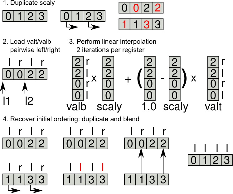
Figure 4: Vectorization of part 2 of the algorithm: The data is loaded pairwise into the vector registers. The interpolation of iterations 0,2 and 1,3 are computed simultaneously. Afterwards the results must be reordered for the second interpolation step.

Note that any further inner loop unrolling beyond what is required by SIMD vectorization would not show any benefit due to register shortage; however, as will be shown later, SMT can be used to achieve a similar effect.

4.2 AVX implementation

In theory, the new AVX instruction set extension doubles the performance per core. The backprojection cannot fully benefit from this advantage because the number of required instructions increases linearly with the register width in part 2 of the algorithm. For arbitrary SIMD vector lengths a hardware gather operation would be required to prevent this part from becoming a severe bottleneck.

Also the limited number of AVX instructions that natively operate on 256-bit registers impedes more sophisticated variants of part 2; only the simple version V1 could be ported. Implementation of V2 would be possible only at the price of a much larger instruction count, so this alternative was not considered. Still an improvement of 25% could be achieved with the AVX kernel on Sandy Bridge (see Sect. 7 for detailed performance results).

Intel already announced the successor AVX2, which will be implemented in the Intel Haswell processor in 2012. AVX2 will fix issues preventing better performance for the backprojection algorithm which are the hardware gather instruction and a more complete instruction set operating on the full SIMD register width.

5 In-depth performance analysis

5.1 Analytic performance model

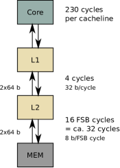
(a) Harpertown

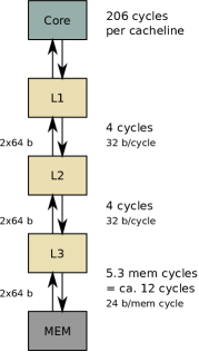
(b) Westmere

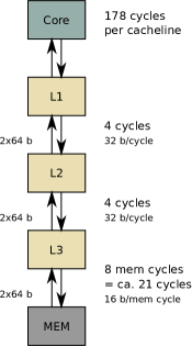
(c) Sandy Bridge (SSE)

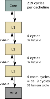
(d) Westmere EX

Figure 5: Performance Analysis: Runtime contributions from instruction execution and necessary cacheline transfers. Each arrow is a 64-byte cacheline transfer. The total data volume in bytes is indicated on the left of each group of arrows. On the right we show the data transfer capabilities between hierarchy levels and the resulting transfer time in core cycles. This assumes that the transfer time is solely determined by bandwidth capabilities, and any latency influence is ignored. For data transfers from main memory the contribution in memory/FSB cycles are translated to core cycles. In-core execution times are measured values from Table 2, scaled to a complete cacheline.

Popular performance models for bandwidth-limited algorithms reduce the influence on the runtime to the algorithmic balance, taking into account the sustained main memory performance [22]. This assumption works well in many cases, especially when there is a large gap between arithmetic capabilities and main memory bandwidth. Recently it was shown [23] that this simplification is problematic on newer architectures like Intel Core i7 because of their exceptionally large memory bandwidth per socket; e.g., a single Nehalem core cannot saturate the memory interface [24]. Moreover the additional L3 cache decouples core instruction execution from main memory transfers and generally provides a better opportunity to overlap data traffic between different levels of the memory hierarchy. Note that in a multithreaded scenario the simple bandwidth model can indeed work as long as multiple cores are able to saturate the socket bandwidth. This property depends crucially on the algorithm, of course.

In [23] we have introduced a more detailed analytic method for cases where the balance model is not sufficient to predict performance with the required accuracy, and the in-cache data transfers account for a significant fraction of overall runtime. This model is based on an instruction analysis of the innermost loop body and runtime contributions of cacheline transfer volumes through the whole memory hierarchy. We first cover single-threaded execution only and then generalize to multithreading on the socket once the basic performance limitations are understood.

A useful starting point for all further analysis is the single-thread runtime spent executing instructions with data loaded from L1 cache. The Intel Architecture Code Analyzer (IACA) [25] was used to analytically determine the runtime of the loop body. This tool calculates the raw throughput according to the architectural properties of the processor under the assumption that all data resides in the L1 cache. It supports Westmere and Sandy Bridge (including AVX) as target architectures. The results for Westmere are shown in the following table for the two SSE kernel variants described above (all entries except $\mu$OPs are in core cycles):

	Issue port
Variant	0	1	2	3	4	5	TP	$\mu$OPs	CP
V1	15	21	24	3	3	19	24	85	54
V2	20	27	16	1	1	20	27	85	71

Execution times are calculated separately for all six issue ports (0…5). (A $\mu$OP is a RISC-like “micro-instruction;” x86 processors perform an on-the-fly translation of machine instructions to $\mu$OPs, which are the “real” instructions that get executed by the core.) Apart from the raw throughput (TP) and the total number of $\mu$OPs the tool also reports a runtime prediction taking into account latencies on the critical path (CP). Based on this prediction V1 should be faster than V2 on Westmere. However, the measurements in Table 2 show the opposite result. The high pressure on the load issue port (2) together with an overall high pressure on all ALU issue ports (0, 1, and 5) seems to be decisive. In V2 the pressure on port 2 is much lower, although the overall pressure on all issue ports is slightly larger.

Below we report the results for the Sandy Bridge architecture with SSE and AVX. The pressure on the ALU ports is similar, but due to the doubled SSE load performance Sandy Bridge needs only half the cycles for the loads in kernel V1. V1 is therefore faster than V2 on Sandy Bridge (see Table 2).

	Issue port
Variant	0	1	2	3	4	5	TP	$\mu$OPs	CP
V1 SSE	16	20	14	13	3	19	20	85	56
V2 SSE	20	26	9	8	1	21	26	85	72
V1 AVX	18	20	22	21	6	30	30	114	90

	HPT	WEM	WEX	SNB
V1 SSE	62.6	61.6	59.6	44.4
V2 SSE	57.4	51.5	54.7	50.0
V1 AVX				76.2

Table 2: Measured execution times (one core) in cycles for one iteration of the SIMD-vectorized kernel (i.e., 4 or 8 voxel updates) with all operands residing in L1 cache.

So far we have assumed that all data resides in the L1 cache. The data transfers required to bring cachelines into L1 and back to memory are modeled separately. We assume that there is no overlap between data transfers and instruction execution. This is true at least for the L1 cache: It can either communicate with L2 to load or evict a cacheline, or it can deliver data to the registers, but not both at the same time. As a first approximation we also (pessimistically) assume that this “no-overlapping” condition holds for all caches, and that a data transfer between any two adjacent levels in the memory hierarchy does not overlap with anything else. Since the smallest transfer unit is a 64-byte cacheline, the analysis will from now on be based on a full “cacheline update” (16 four-byte voxels), which corresponds to four (two) inner loop iterations when using SSE (AVX).

We only consider the data traffic for voxel updates; the image data traffic is negligible in comparison, hence we assume that all image data comes from L1 cache. It takes two cycles to transfer one cacheline between adjacent cache levels over the 256-bit unidirectional data path. Every modified line must eventually be evicted, which takes another two cycles. Figure 5 shows a full analysis, in which the core execution time for a complete cacheline update is based on the measured cycles from Table 2. On the three architectures with L3 cache the simplification is made that the “Uncore” part (L3 cache, memory interface, and QuickPath interconnect) runs at the same frequency as the core, which is not strictly true but does not change the results significantly. It was shown for the Nehalem-based architectures (Westmere and Westmere EX) that they can overlap instruction execution with reloading data from memory to the last level cache [24]. Hence, the model predicts that the in-core execution time is much larger than all other contributions, which makes this algorithm limited by instruction throughput for single core execution. On Sandy Bridge, the AVX kernel requires 76.2 cycles for one vectorized loop iteration (eight updates). This results in 152 cycles instead of 178 cycles (SSE) for one cacheline update.

Based on the runtime of the loop kernel we can now estimate the total required memory bandwidth for multithreaded execution if all cores on a socket are utilized, and also derive the expected performance (we consider the full volume without clipping):

	HPT	WEM	WEX	SNB	SNB (AVX)
BW/core [GB/s]	1.7	1.9	1.5	2.5	3.0
BW/socket [GB/s]	6.8	11.2	11.6	10.0	12.0
Perf. [GUP/s]	0.85	1.42	1.45	1.25	1.51

We conclude that the multithreaded code is bandwidth-limited only on Harpertown, since the required socket bandwidth is above the practical limit given by the update benchmark (see Table 1). All other architectures are below their data transfer capabilities for this operation and should show no benefit from further bandwidth-reducing optimizations (see Sect. 6.2).

5.2 ILP optimization and SMT

At this point the analysis still neglects the possible benefit from SMT. SMT can significantly improve the efficiency of the floating point units for codes that are limited by instruction throughput and suffer from underutilization of the arithmetic units due to dependencies or instruction scheduling issues. This is definitely the case here, as indicated by the discrepancy between the “throughput” and “critical path” predictions in the previous section. Due to the complex loop body register dependencies are unavoidable, resulting in many pipeline bubbles. Outer loop unroll and jam (interleaving two outer loop iterations in the inner body) is out of the question due to register shortage, but SMT can do a similar job and provide independent instruction streams using independent register sets. Since memory bandwidth is no limitation on all SMT-enabled processors considered here, running two threads on the two virtual cores of each physical core is expected to reduce the cycles taken for the cacheline update. However, the effect of using SMT is difficult to estimate quantitatively. See Sect. 7 below for complete parallel results

6 OpenMP parallelization

OpenMP parallelization of the algorithm is straightforward and works with all optimizations discussed so far. For the thread counts and problem sizes under consideration here it is sufficient to parallelize the loop that iterates over all voxel volume slices (loop variable z in Listing 1). However, due to the clipped-off voxels at the edges and corners of the volume, simple static loop scheduling with default chunksize leads to a strong load imbalance. This can be easily corrected by using block-cyclic scheduling with a small chunksize (e.g., static,1).

Images are produced one by one during the C-arm rotation, and could at best be delivered to the application in batches. Since the reconstruction should start as soon as images become available, a parallelization across images was not considered.

As shown in Sect. 5, the socket-level performance analysis does not predict strong benefits from bandwidth-reducing optimizations except on the Harpertown platform. However, since one can expect to see more bandwidth-starved processor designs with a more unbalanced ratio of peak performance to memory bandwidth in the future, we still consider bandwidth optimizations important for this algorithm. Furthermore, ccNUMA architectures have become omnipresent even in the commodity market, making locality and bandwidth awareness mandatory. In the following sections we will describe a proper ccNUMA page placement strategy for voxel and image data, and a blocking optimization for bandwidth reduction. The reason why we present those optimizations in the context of shared-memory parallelization is that they become relevant only in the parallel case, since bandwidth is not a problem on all architectures for serial execution (see Sect. 5.1).

6.1 ccNUMA placement

The reconstruction algorithm uses essentially two relevant data structures: the voxel array and the image data arrays. Upon voxel initialization one can easily employ first-touch initialization, using the same OpenMP loop schedule (i.e., access pattern) as in the main program loop. This way each thread has local access (i.e., within its own ccNUMA domain) to its assigned voxel layers, and the full aggregate bandwidth of a ccNUMA node can be utilized.

Although the access to the projection image data is much less bandwidth-intensive than the memory traffic incurred by the voxel updates, ccNUMA page placement was implemented here as well. As mentioned in Sect. 3.3, the padded projection buffers are explicitly allocated and initialized in each locality domain, and a local copy is shared by all threads within a domain. Since the additional overhead for the duplication is negligible, this ensures conflict-free local access to all image data. The time taken to copy the images to the local buffers is included in the runtime measurements.

6.2 Blocking/unrolling

In order to reduce the pressure on the memory interface we use a simple blocking scheme for the outer loop over all images: Projections are loaded and copied to the padded projection buffers in small chunks, i.e., $b$ images at a time. The line update kernel (see Sect. 4) for a certain pair of $(y,z)$ coordinates is then executed $b$ times, once for each projection. This corresponds to a $b$-way unrolling of the image loop and a subsequent jam into the next-to-innermost voxel loop (across the $y$ voxel coordinate). At the problem sizes studied here, all the voxel data for this line can be kept in the L1 cache and reused $b-1$ times. Hence, the complete volume is only updated in memory $496/b$ instead of 496 times. Relatively small unrolling factors between $2$ and $8$ are thus sufficient to reduce the bandwidth requirements to uncritical levels even on “starved” processors like the Intel Harpertown.

This optimization is so effective that it renders proper ccNUMA placement all but obsolete; we will thus not report the benefit of ccNUMA placement in our performance results, although it is certainly performed in the code.

7 Results

In order to evaluate the benefit of our optimizations we have benchmarked different code versions with the $512^{3}$ case on all test machines. RabbitCT includes a benchmarking application, which takes care of timing and error checking. It reports total runtime in seconds for the complete backprojection. We performed additional hardware performance counter measurements using the likwid-perfctr tool. Likwid-perfctr can produce high-resolution timelines of counter data and useful derived metrics on the core and node level without changes to the source code. Unless stated otherwise we always report results using two SMT threads per core. For all architectures apart from Sandy Bridge the line update kernel version V2 was used. On Sandy Bridge results for the SSE kernel V1 as well as for the AVX port of the V1 kernel are presented.

7.1 Validation of analytical predictions

To validate the predicted performance of the analytic model (see Sect. 5), single-socket runs were performed without the clipping optimization and SMT. Blocking was used on the Harpertown platform only, to ensure that execution is not dominated by memory access. The following table shows the measured performance and the deviation against the model prediction:

	HPT	WEM	WEX	SNB	SNB (AVX)
Perf. [GUP/s]	0.75	1.20	1.30	1.11	1.28
deviation	-13.3%	-18.3%	-11.5%	-12.6%	-18.0%

This demonstrates that the model has a reasonable predictive power. It has been confirmed that the contribution of data transfers indeed vanishes against the core runtime, despite the fact that the total transfer volume is high and a first rough estimate based on data transfers and arithmetic throughput alone (Sect. 3) predicted a bandwidth limitation of this algorithm on all machines.

As a general rule, the IACA tool can provide a rough estimate of the innermost loop kernel runtime via static code analysis. Still it is necessary to further enhance the machine model to improve the accuracy of the predictions. Especially the ability of the out of order scheduler to exploit superscalar execution was overestimated and has led to qualitatively wrong predictions.

Note that this example is an extreme case with all data transfers vanishing against core runtime. However, the approach also works for bandwidth-limited codes, as was shown in [23].

7.2 Impact of optimizations on accuracy

One of the costly operations in this algorithm is the divide involved. A possible optimization is to use the fully pipelined reciprocal (rcpps), which provides an approximation with 12-bit accuracy compared to the 24-bit accuracy of the regular divide instruction. The accuracy of the reciprocal can be improved to at least 21 bits using a Newton-Raphson iteration [26]. This requires four additional arithmetic instructions in the implementation. The following table shows the peak signal-to-noise ratio (PSNR) and performance of the three alternatives: Regular divide instruction, reciprocal, and reciprocal with Newton-Raphson iteration, on the Westmere test machine for the fully optimized case (full node).

	Performance [GUP/s]	PSNR [dB]
divps	3.79	103
rcpps	4.21	67.7
Newton-Raphson	3.79	103

As usual in image processing, the PSNR was determined as the logarithm of a mean quadratic deviation from a reference image:

$$\mbox{PSNR}=10\cdot\log_{10}\frac{M^{2}}{\displaystyle L^{-3}\sum_{x,y,z}\left[V(x,y,z)-R(x,y,z)\right]^{2}}$$ (1)

Here $V(x,y,z)$ is the reconstructed voxel grayscale value at coordinates $(x,y,z)$ scaled to the interval $[0,M]$, and $R(x,y,z)$ is a reference voxel with the “correct” result. The higher the PSNR, the more accurate the reconstruction.

There is no significant difference neither in performance nor accuracy between the regular divide and rcpps with Newton-Raphson. The performance improvement when using rcpps alone is 10%, at an accuracy which is still better than for the published GPGPU implementations (63–65 dB). In the following section we discuss performance results using this latter version.

7.3 Parallel results

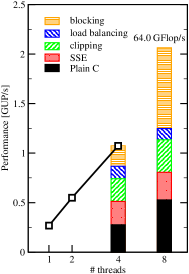
(a) Harpertown

(b) Sandy Bridge

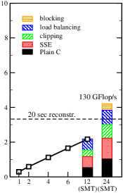
(c) Westmere

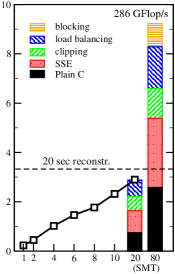
(d) Westmere EX

Figure 6: Scalability and performance results for the $512^{3}$ test case on all platforms. In-socket scalability was tested using the best version of the SIMD-vectorized line update kernel on each system (AVX-V1 on Sandy Bridge, SSE-V2 on all others). The practical performance goal for complete reconstruction (20 seconds runtime, corresponding to 3.33 GUP/s) is indicated as a dashed line. Gflop/s numbers have been computed assuming 31 flops per optimized (scalar) inner loop iteration. Note the scale change between the left and right pairs of graphs.

Figures 6 (a)–(d) display a summary of all performance results on node and socket levels, and parallel scaling inside one socket for the best version on each architecture. All machines show nearly ideal scaling inside one socket when using physical cores only. With SMT, the benefit is considerable on Sandy Bridge (33%) and Westmere (31%), and a little smaller on Westmere EX (25%). The large effect on Sandy Bridge may be attributed to a higher number of bubbles in the pipeline, as indicated by the larger discrepancy between the “throughput” and “critical path” cycles in the AVX loop kernel (see Sect. 5.2). Scalability from one to all sockets of the node is also close to perfect for the multisocket machines, with the exception of Westmere EX, on which there is a slight load imbalance due to 80 threads working on only 512 slices.

(a) OpenMP static scheduling

(b) OpenMP cyclic (static,1) scheduling

Figure 7: Timeline view of the L2 to L1 cacheline traffic for three cores of a 6-thread run without clipping on one Westmere socket, using (a) standard static OpenMP scheduling and (b) cyclic “static,1” scheduling.

Depending on the architecture, SSE vectorization boosts performance by a factor of 2–3 on the socket level. As explained earlier (see Sect. 4), part 2 of the algorithm prohibits the optimal speedup of 4 because its runtime is linear in the SIMD vector length. Work reduction through clipping alone shows only limited effect due to load imbalance, but this can be remedied by an appropriate cyclic OpenMP scheduling, as described in Sect. 6. This kind of load balancing not only improves the work distribution but also leads to a more similar access pattern to the projection images across all threads. This can be seen in Fig. 7 (a), which shows the cacheline traffic between the L2 and L1 cache during a 6-thread run on one Westmere socket with all optimizations except clipping (only 3 cores are shown for clarity). Although the amount of work, i.e., the number of voxels, is perfectly balanced across all threads, there is a strong discrepancy in cacheline traffic between threads when standard static scheduling is used. The reason for this is that the projections of voxel lines onto the detector are quite different for lines that are far apart from each other in the volume, which leads to vastly different access patterns to the image data, and hence very dissimilar locality properties. Cyclic scheduling removes this variation (see Fig. 7 (b)).

Cache blocking has little to no effect on all architectures except Harpertown, as predicted by our analysis. Fig. 8 shows timelines for socket floating point performance and bandwidth on one Westmere socket, comparing blocked/nonblocked and SMT/non-SMT variants. Fig. 8 (a) clearly demonstrates the performance boost of SMT in contrast to the very limited effect of blocking. On the other hand, the blocked implementation significantly reduces the bandwidth requirements (Fig. 8 (b)). The blocked variants have a noticeable amplitude of variations while the nonblocked versions appear smooth. In the inset of Fig. 8 (b) we show a zoomed-in view with finer time resolution, which indicates that the frequency of bandwidth variations is much larger without blocking; this is plausible since the bandwidth is dominated by the voxel volume in this case. With blocking, individual voxel lines are transferred in “bursts” with phases of inactivity in between, where image data is read at low bandwidth.

The benefit of AVX on Sandy Bridge falls short of expectations for the same reason as in the SSE case. Still it is remarkable that the desktop Sandy Bridge system outperforms the dual-socket Harpertown server node, which features twice the number of cores at a similar clock speed. Both Westmere and Westmere EX meet the performance requirements of at most 20 sec for a complete volume reconstruction. The Westmere EX node is, however, not competitive due to its unfavorable price to performance ratio. It is an option if absolute performance is the only criterion.

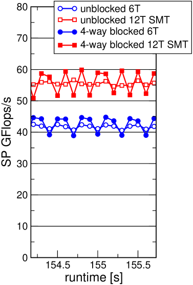
(a) FP performance

(b) Memory bandwidth

Figure 8: Performance counter timeline monitoring of floating-point performance (a) and memory bandwidth (b), comparing blocked/nonblocked and SMT/non-SMT variants of the best implementation on one Westmere socket at 100 ms resolution. The inset in (b) shows a zoomed-in view with 2 ms resolution.

8 CPU vs. GPGPU

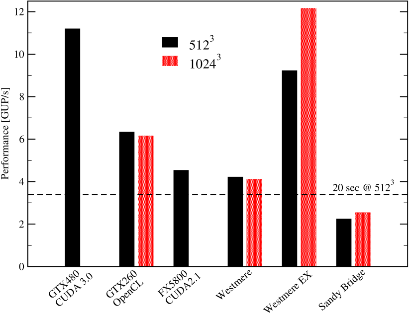
Figure 9: Performance comparison between the best reported GPGPU implementations in OpenCL and CUDA and our CPU versions on the systems in the test bed for problem sizes $512^{3}$ and $1024^{3}$, respectively. There is currently no working CUDA implementation for the latter case. The practical performance goal for complete reconstruction of a $512^{3}$ volume (3.33 GUP/s) is indicated by a dashed line.

Since the backprojection algorithm is well suited for GPGPUs, the performance leaders of the open competition benchmark have traditionally been GPGPU implementations in OpenCL and CUDA. The gap to the fastest CPU version reported on the RabbitCT Web site [9] before this work was started was very large. For the reasons given in the derivation of the performance model, simple bandwidth or peak performance comparisons are inadequate to estimate the expected reconstruction speed advantage of GPGPUs, although it should certainly lie inside the usual corridor of 4–10 when comparing with a full CPU socket. An example of a well-optimized GPU code was published recently [27]. Our implementation shows that current x86 multicore chips are truly competitive (see Fig. 9), even when considering the price/performance ratio. Beyond the clinically relevant $512^{3}$ case, industrial applications need higher resolutions. This is a problem for GPGPU implementations because the local memory on the card is often too small to hold the complete voxel volume, causing extra overhead for moving partial volumes in and out of the local memory and leading to a more complex implementation. If the price for the hardware is unimportant, a Westmere EX node is an option that can easily outperform GPGPUs. Note that the unusually large gap between the performance levels at $512^{3}$ and $1024^{3}$ on this architecture may be attributed to better load balancing when 80 threads work on 1024 instead of 512 slices. It also lifts the performance efficiency (fraction of node peak) on this system to about 50%, matching the level achieved by the other multicore nodes already on the smaller problem. This compares to 26% for the CUDA code on the GTX480 card, assuming the same number of flops per voxel update.

The results for the Sandy Bridge desktop system and the good scalability even of the optimized algorithm promise even better performance levels on commodity multicore systems in the future. Note that it would be possible to provide a simple and efficient distributed memory parallelization of the algorithm for even faster reconstruction. “Micro-clusters” based on cheap desktop technology could then easily meet any time constraint at extremely low cost. However, a comparison based on the hardware cost alone is certainly too simplistic, especially when taking into account the overall cost for a complete CT scanner including maintenance.

9 Conclusions and Outlook

We have demonstrated several algorithmic and low-level optimizations for a CT backprojection algorithm on current Intel x86 multicore processors. Highly optimizing compilers were not able to deliver useful SIMD-vectorized code. Our implementation is thus based on assembly language and vectorized using the standard instruction set extensions SSE and AVX. The results show that commodity hardware can be competitive with highly tuned GPU implementations for the clinically relevant $512^{3}$ voxel case at the same level of accuracy. Nonpipelined divide instructions (divps) or a fast pipelined version (rcpps) with subsequent Newton-Raphson iteration provide better accuracy at a 10% performance penalty. Our results showed that it is necessary to consider all aspects of processor and system architecture in order to reach best performance, and that the effects of different optimizations are closely connected to each other. The benefit of the AVX instruction set on Sandy Bridge was limited due to the lack of a gathered load and the small number of instructions that natively operate on the full SIMD register width. This relevant algorithm can achieve very good efficiencies on commodity processors and it would be a natural step to further improve performance with a distributed memory implementation. At higher resolutions, which are used in industrial applications, multicore systems are frequently the only choice (apart from expensive custom solutions).

Future work includes a more thorough analysis and optimization of the AVX line update kernel, and an inclusion of the new AVX2 gather operations once they become available.

10 Acknowledgments

We are indebted to Intel Germany for providing test systems and early access hardware for benchmarking. This work was supported by the Competence Network for Scientific High Performance Computing in Bavaria (KONWIHR) under project OMI4papps.

References

- [1] A. Kak and M. Slaney. Principles of Computerized Tomographic Imaging (SIAM), 2001.
- [2] N. Strobel and et al. 3D Imaging with Flat-Detector C-Arm Systems. In: Multislice CT (Springer, Berlin / Heidelberg), 3rd ed. ISBN 978-3-540-33125-4, 33–51.
- [3] L. Feldkamp, L. Davis and J. Kress. Practical Cone-Beam Algorithm. Journal of the Optical Society of America A1(6), (1984) 612–619.
- [4] B. Heigl and M. Kowarschik. High-speed reconstruction for C-arm computed tomography. In: 9th International Meeting on Fully Three-Dimensional Image Reconstruction in Radiology and Nuclear Medicine (www.fully3d.org, Lindau), 25–28.
- [5] K. Mueller and R. Yagel. Rapid 3D cone-beam reconstruction with the Algebraic Reconstruction Technique (ART) by utilizing texture mapping graphics hardware. Nuclear Science Symposium, 1998. Conference Record. 3, (1998) 1552–1559.
- [6] K. Mueller, F. Xu and N. Neophytou. Why do Commodity Graphics Hardware Boards (GPUs) work so well for acceleration of Computed Tomography? In: SPIE Electronic Imaging Conference, vol. 6498 (San Diego), 64980N.1–64980N.12.
- [7] H. Scherl, M. Koerner, H. Hofmann, W. Eckert, M. Kowarschik and J. Hornegger. Implementation of the FDK algorithm for cone-beam CT on the cell broadband engine architecture. In: J. Hsieh and M. J. Flynn (eds.), SPIE Medical Imaging Conference Proc., vol. 6510 (SPIE), 651058.
-
[8]
C. Rohkohl, B. Keck, H. G. Hofmann and J. Hornegger.
RabbitCT—An Open Platform for Benchmarking 3-D
Cone-beam Reconstruction Algorithms.
Medical Physics 36(9), (2009) 3940–3944.
http://link.aip.org/link/?MPH/36/3940/1 - [9] RabbitCT Benchmark. http://www.rabbitct.com/.
- [10] H. G. Hofmann, B. Keck, C. Rohkohl and J. Hornegger. Comparing Performance of Many-core CPUs and GPUs for Static and Motion Compensated Reconstruction of C-arm CT Data. Medical Physics 38(1), (2011) 3940–3944.
- [11] H. Kunze, W. Härer and K. Stierstorfer. Iterative extended field of view reconstruction. In: J. Hsieh and M. J. Flynn (eds.), Medical Imaging 2007: Physics of Medical Imaging., vol. 6510 of Society of Photo-Optical Instrumentation Engineers (SPIE) Conference Series (San Diego), 65105X.
- [12] C. Rohkohl, G. Lauritsch, M. Prümmer and J. Hornegger. Interventional 4-D Motion Estimation and Reconstruction of Cardiac Vasculature without Motion Periodicity Assumption. In: G.-Z. Yang, D. Hawkes, D. Rueckert, A. Noble and C. Taylor (eds.), Medical Image Computing and Computer-Assisted Intervention – MICCAI 2009, vol. 5761 of Lecture Notes in Computer Science (Springer, Berlin / Heidelberg). ISBN 978-3-642-04267-6, 132–139.
-
[13]
B. Keck, H. Hofmann, H. Scherl, M. Kowarschik and J. Hornegger.
High Resolution Iterative CT Reconstruction using Graphics
Hardware.
In: B. Yu (ed.), 2009 IEEE Nuclear Science Symposium
Conference Record (N/A), 4035–4040.
http://www5.informatik.uni-erlangen.de/Forschung/Publik%ationen/2009/Keck09-HRI.pdf - [14] Intel. Intel advanced vector extensions programming reference, Apr 2011.
- [15] Intel many integrated core architecture. http://www.intel.com/technology/architecture-silicon/mic/index.htm.
- [16] Godson 3b architecture. http://www.theregister.co.uk/2011/02/25/ict\_godson\_3b\_chip/page2.htm%l, Feb 2011.
- [17] The Stream Benchmark. http://www.streambench.org/.
- [18] J. Treibig, G. Hager and G. Wellein. Likwid: A lightweight performance-oriented tool suite for x86 multicore environments. In: Proceedings of PSTI2010, the First International Workshop on Parallel Software Tools and Tool Infrastructures (San Diego CA).
-
[19]
LIKWID performance tools.
http://code.google.com/p/likwid - [20] I. Goddard, A. Berman, O. Bockenbach, F. Lauginiger, S. Schuberth and S. Thieret. Evolution of computer technology for fast cone beam backprojection. In: Society of Photo-Optical Instrumentation Engineers (SPIE) Conference Series, vol. 6498.
-
[21]
H. G. Hofmann, B. Keck and J. Hornegger.
Accelerated C-arm Reconstruction by Out-of-Projection
Prediction.
In: T. M. Deserno, H. Handels, H.-P. Meinzer and T. Tolxdorff (eds.),
Bildverarbeitung für die Medizin 2010 (Berlin).
ISBN 978-3-642-11967-5, 380–384.
http://www5.informatik.uni-erlangen.de/Forschung/Publik%ationen/2010/Hofmann10-ACR.pdf - [22] G. Hager and G. Wellein. Introduction to High Performance Computing for Scientists and Engineers (CRC Press), 2010. ISBN 978-1439811924.
-
[23]
J. Treibig and G. Hager.
Introducing a performance model for bandwidth-limited loop
kernels.
In: Proceedings of the Workshop Memory issues on Multi- and
Manycore Platforms at PPAM 2009, the 8th International Conference on Parallel
Processing and Applied Mathematics (Wroclaw Poland).
http://arxiv.org/abs/0905.0792 - [24] J. Treibig, G. Hager and G. Wellein. Complexities of performance prediction for bandwidth-limited loop kernels on multi-core architectures. In: High Performance Computing in Science and Engineering (Springer, Berlin / Heidelberg, Garching/Munich). ISBN 978-3642138713.
-
[25]
Intel.
Intel architecture code analyzer, Apr 2011.
http://software.intel.com/en-us/articles/intel-architec%ture-code-analyzer/ - [26] Intel. Ap-803 increasing the accuracy of the results from the reciprocal and reciprocal square root instructions using the newton-raphson method, Apr 1999.
- [27] E. Papenhausen, Z. Zheng and K. Mueller. GPU-Accelerated Back-Projection Revisited: Squeezing Performance by Careful Tuning. Workshop on High Performance Image Reconstruction (HPIR), 2011.