A Data Cube Extraction Pipeline for a
Coronagraphic Integral Field Spectrograph

Abstract

Project 1640 is a high contrast near-infrared instrument probing the vicinities of nearby stars through the unique combination of an integral field spectrograph with a Lyot coronagraph and a high-order adaptive optics system. The extraordinary data reduction demands, similar those which several new exoplanet imaging instruments will face in the near future, have been met by the novel software algorithms described herein. The Project 1640 Data Cube Extraction Pipeline (PCXP) automates the translation of $3.8\times 10^{4}$ closely packed, coarsely sampled spectra to a data cube. We implement a robust empirical model of the spectrograph focal plane geometry to register the detector image at sub-pixel precision, and map the cube extraction. We demonstrate our ability to accurately retrieve source spectra based on an observation of Saturn’s moon Titan.

1 Introduction

In recent years an assortment of new astronomical techniques have evolved to address the challenges of imaging faint objects and disk structure at close angular separations to nearby stars. A major scientific motivation for these efforts is the direct detection and characterization of low-mass companion bodies orbiting at separations between $\sim$ 5 and 100 AU. These objects are beyond the reach of conventional optical imaging due to the extreme contrast in brightness with respect to the primary star. In such cases, even under ideal observing conditions the diffracted light of the primary star overwhelms the neighboring source of interest. The various methods of manipulating a star’s light to enable investigation of its immediate environment are collectively referred to as high-contrast imaging. For a recent review of this field, see Oppenheimer & Hinkley (2009). The acquisition of spectra of young, sub-stellar mass objects in this newly opened parameter space will ultimately lead to a breakthrough in our understanding of exoplanet populations (Beichman et al., 2010).

Project 1640 (P1640) is the first of several instruments to approach the high contrast imaging problem through a combination of high-order adaptive optics, a Lyot coronagraph, and an integral field spectrograph (Hinkley et al., 2011). Forthcoming instruments using a similar design include the Gemini Planet Imager (GPI) (Macintosh et al., 2006), the Very Large Telescope Spectro-Polarimetric High-contrast Exoplanet REsearch (VLT-SPHERE) project (Beuzit et al., 2008), and the Subaru Telescope Planetary Origins Imaging Spectrograph (POISE) (McElwain et al., 2008). While previous efforts have used integral field spectrographs for high contrast imaging (e.g. Thatte et al., 2007; McElwain et al., 2007; Janson et al., 2008), and Lyot coronagraphs have also been employed for surveys of nearby stars (e.g. Chauvin et al., 2010; Leconte et al., 2010), P1640 is the first instrument to combine these two technologies. The coronagraph component, based on the Fourier optics concept described in Sivaramakrishnan et al. (2001), rejects the core of the target star’s point spread function (PSF) and attenuates the surrounding diffraction rings. Provided that the adaptive optics (AO) system upstream of the coronagraph has corrected the star’s PSF to near the diffraction limit, then the dominant source of noise in the image exiting the coronagraph takes the form of a halo of speckles surrounding the occulted star, as in Figure 1 (Racine et al., 1999; Perrin et al., 2003). These relatively long-lived, point source-like artifacts are caused by uncorrected wave front aberrations, and limit the dynamic range of the data unless further processing is carried out (Hinkley et al., 2007).

The integral field spectrograph, also referred to as the integral field unit (IFU), is situated after the coronagraph and provides spatially resolved spectra for a grid of points across the field of view (Bacon et al., 1988). The reduced form of data acquired with an IFU is a stack of simultaneous narrowband images spanning the instrument’s wavelength range, often called a data cube. An example of part of a P1640 data cube is shown in Figure 1. One benefit the IFU provides is enabling the observer to measure the spectrum of any source at any position in the field of view. This is not possible with a conventional spectrograph, which can only use one spatial dimension at a time to discriminate against other sources in the field of view. The second purpose of the IFU is to exploit the chromatic behavior of the speckles (Sparks & Ford, 2002). Speckles are optical in origin and their separation from the target star is linearly proportional to wavelength, at least to a first-order approximation (see Figure 1). By comparing the images in different channels of the data cube, the observer can discriminate the speckles from a true point source, whose position should remain constant with wavelength. Furthermore, automated post-processing software can use the chromaticity of the speckles to subtract a large component of them from the data, taking a reduced data cube as input and generating a speckle-suppressed version (Crepp et al., 2011; Pueyo et al., 2011).

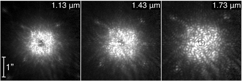
Figure 1: Three of the 23 channels making up an example P1640 data cube, formed from a 154 s exposure of the coronagraphically occulted star HD 27946 ($V$ = 5.3). The three channel images shown here, each consisting of $200\times 200$ spaxels, are displayed with a square root stretch. A halo of well-defined speckles surround the focal plane mask, expanding with wavelength. The cube configuration of the data enables post-processing algorithms to take advantage of the chromaticity of speckles to reduce their influence on detection limits.

The unusual properties of data generated by the P1640 IFU necessitate novel reduction techniques to reach the point where inspection, spectrophotometry, astrometry, and advanced post-processing techniques like speckle suppression can begin. In the scope of this article, we describe the software created to translate rapidly the raw data from the IFU camera to a set of data cubes ready for further analysis.

2 Project 1640 Design and Data Acquisition

During operation at Palomar Observatory, P1640 receives a wave front-corrected beam of the target star’s light from the 200” Hale Telescope AO system. The current AO system, the 241-actuator PALAO (Dekany et al., 1997), will soon be upgraded to the 3388-actuator PALM-3000 (Bouchez et al., 2009). Upon entering the instrument, the light passes through an apodized Lyot coronagraph, followed by an integral field spectrograph, which contains a near-infrared camera.

In addition to the focal plane mask and Lyot stop of a traditional Lyot coronagraph, P1640 uses a pupil plane apodization mask to optimize the starlight suppression based on the telescope pupil shape (Soummer, 2005). The beam exiting the coronagraph comes to a focus on a $200\times 200$ square microlens array at the entrance of the spectrograph. Immediately after the microlens array, the light is collimated to form a pupil on a wedge-shaped prism, which disperses the light over the 1.1-1.8 $\mu$m wavelength range of operation spanning the $J$ and $H$ bands. Additional optics focus the $4\times 10^{4}$ resulting spectra onto a Teledyne HAWAII-2 $2048\times 2048$ pixel, HgCdTe, near-infrared detector. The field of view of the final image, designed to match the control radius of the PALM-3000 AO system, is $4\arcsec\times 4\arcsec$. For further details on the optical and mechanical design, see Hinkley et al. (2011).

For each exposure, the camera controller performs a sequence of non-destructive reads on the detector array. In other words, the digitized value of each pixel is periodically sampled while its voltage escalates. This technique, known as up-the-ramp sampling, can result in the read noise being reduced by a factor of $\sqrt{N/12}$ in a reduced image when the counts versus read slope is fit for the $N$ samples of each pixel (Offenberg et al., 2001). Up-the-ramp sampling also adds an advantageous temporal dimension to our data. Speckle suppression algorithms work best when the positions of the speckles are well-defined. For bright stars with high signal-to-noise in individual read differences, it may be helpful to “freeze” the speckle pattern with the higher time resolution enabled in a read-by-read data reduction. Our pipeline reduces the detector data with both approaches: the non-destructive read (NDR) slope fit and consecutive read differences.

The read sample interval is fixed at 7.7 seconds by the camera controller. The sequence of reads are stored in a binary file containing the arrays of 16-bit unsigned integer samples, which we refer to as a dat file. The camera controller also generates a separate FITS file with a header containing the information about the telescope and instrument status, the target (coordinates, magnitude, parallax, etc.), and the name of the dat file corresponding to the exposure. A typical observation of a Project 1640 science target is made up of 15 exposures, each containing 20 reads, giving a cumulative exposure time of $38.6$ minutes. The resulting volume of raw data is 160 Mbytes for each exposure’s dat file and 2.4 Gbytes in total.

The structure of the P1640 IFU focal plane, illuminated by Moonlight, is depicted in Figure 2. The microlens array, represented by the dotted grid superimposed on the left panel, is rotated with respect to the detector. This configuration interleaves the adjacent rows of microlens spectra, thereby maximizing the efficiency of focal plane area usage. Along a given column of microlenses, the mean interval between neighboring spectra is 3.3 pixels in the horizontal direction and 10.0 pixels in the vertical direction. Each spectrum takes up a length of approximately 27 pixels in the dispersion direction.

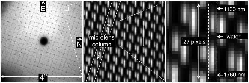
Figure 2: A hierarchical diagram of the P1640 integral field spectrograph focal plane. Left: an average of ten calibration Moon exposures, recorded by the near-infrared detector at the spectrograph focal plane. The projection of the IFU microlens array onto the detector is represented by a superimposed dotted grid, with each gap spanning ten microlenses. Middle: expanding a $100\times 100$ pixel section reveals the underlying pattern of microlens spectra. The tilt of the square microlens array with respect to the detector ($-18.5^{\circ}$) interleaves the adjacent rows of spectra for an efficient use of detector area. Right: each spectrum, spanning $J$ and $H$ band (1.1 $\mu$m to 1.8 $\mu$m), displays the prominent telluric water absorption trough centered near 1.4 $\mu$m.

3 Spectrograph Focal Plane Model

Rather than relying purely on design predictions, we have written procedures to empirically determine the IFU response, capturing the minute optical distortions and alignment changes unique to each observing run. Two forms of calibration data are used as input for the focal plane model. The first kind are the spectrograph images formed by illuminating the instrument pupil with a tunable laser source. These allow us to characterize the response at fixed wavelengths across the passband. Secondly, during each observing run we observe a broadband source of nearly uniform brightness across our field of view—either the Moon or the twilight sky. In the case of the Moon calibration images, the telescope AO correction loop was turned off, and several exposures with different pointings were averaged. These images constrain the geometry of the focal plane, including the positions and shapes of the individual spectra formed on the detector, as well as large-scale variations in sensitivity across the field of view due to vignetting.

3.1 Spectrograph Point Spread Function Model

An accurate model of the monochromatic spectrograph point spread function (PSF) is at the core of the IFU focal plane model. We emphasize the distinction here from the coronagraph PSF, which is formed on the mircolens array at the entrance of the IFU. The spectrograph PSF, on the contrary, is the signal formed on the IFU focal plane from monochromatic light incident on an individual microlens. In a laboratory environment before the first scientific observing run, we illuminated the IFU with a tunable laser source and recorded narrowband emission (bandwidth $<$ 4 nm) images at wavelengths in 0.01 $\mu$m increments spanning the 0.7 $\mu$m operating band of the instrument. Any given laser image shows a grid of $3.8\times 10^{4}$ point spread functions, each corresponding to a microlens illuminated by the beam entering the spectrograph. From these images, we derived an analytic model of the spectrograph PSF specific to the recorded wavelength, as follows: First, a script looped through all of the PSFs in the spectrograph image, forming a 9$\times$9 pixel mean PSF based on the subset having centroids within 0.05 pixels of a detector pixel center. Next, we experimented with a variety of two-dimensional functional forms to represent the PSF, progressively adding parameters until finding one with a good match to the data. Since in our case the detector pixel width is comparable to the PSF full-width half maximum value, it was necessary to take into account not only the effect of the finite detector pixel area in sampling the function, but also intra-pixel sensitivity variations.

Charge diffusion is the largest contribution to non-uniform sensitivity within any given pixel. During the technology development phase of a space mission to survey extragalactic supernovae, Brown (2007) measured the effect of charge diffusion on the intra-pixel sensitivity of a HAWAII-2 detector. He found a good empirical fit to a typical pixel’s response by convolving a tophat function (with width equal to that of the detector pixel) with a hyperbolic secant diffusion term, $\operatorname{sech}(\frac{r}{l_{d}})$, where r is radius from origin and $l_{d}$ is the diffusion length. With the established diffusion length of 1.9 $\mu$m (compared to the 18 $\mu$m full pixel width), the response falls to about 50% of the peak at the middle of each pixel edge. For lack of similar measurements of our own HAWAII-2 detector, we assumed the same charge diffusion behavior.

We discretized the two-dimensional functions representing the PSF, $\mathcal{P}_{M}(u,v)$, and intra-pixel response, $\mathcal{R}_{M}(i,j)$, at a resolution of $M$ times that of the detector, where $M$ is an odd number $\geq$ 3. In other words, the image model has $M\times M$ samples contained within each detector pixel, one always aligned with the center of a pixel. The intra-pixel response function, $\mathcal{R}_{M}$, is only defined over an area of one pixel, so that $i,j\in\{0,1,\dotsc,M-1\}$, whereas $\mathcal{P}_{M}$ is defined over the entire $9M\times 9M$ area of the mean PSF cutout, corresponding to $u,v\in\{0,1,\dotsc,9M-1\}$. In this notation, the detector-downsampled PSF, $\mathbb{P}(x,y)$ is determined by

$$\mathbb{P}(x,y)=\sum_{i=0}^{M-1}\sum_{j=0}^{M-1}\mathcal{P}_{M}(i+Mx,j+My)\mathcal{R}_{M}(i,j)$$ (1)

where $x,y\in\{0,1,\dotsc,8\}$ are independent variables representing detector samples over the $9\times 9$ pixel mean PSF cutout.

We found a satisfactory functional form to match the monochromatic PSF by taking the sum of two piecewise, two-dimensional Gaussian profiles, defined as follows:

$$\mathcal{P}_{M}(u,v)=\left\{\begin{array}[]{lr}Ae^{-\left(\frac{r(u,v)^{2}}{2\sigma^{2}_{A,r}}+\frac{s(u,v)^{2}}{2\sigma^{2}_{A,s+}}\right)}+Be^{-\left(\frac{r(u,v)^{2}}{2\sigma^{2}_{B,r}}+\frac{s(u,v)^{2}}{2\sigma^{2}_{B,s+}}\right)}&s>0\\ Ae^{-\left(\frac{r(u,v)^{2}}{2\sigma^{2}_{A,r}}+\frac{s(u,v)^{2}}{2\sigma^{2}_{A,s-}}\right)}+Be^{-\left(\frac{r(u,v)^{2}}{2\sigma^{2}_{B,r}}+\frac{s(u,v)^{2}}{2\sigma^{2}_{B,s-}}\right)}&s\leq 0\end{array}\right.$$ (2)

where

$$\begin{bmatrix}r\\ s\end{bmatrix}=\begin{bmatrix}\cos\theta&\sin\theta\\ -\sin\theta&\cos\theta\end{bmatrix}\begin{bmatrix}\frac{1}{M}\left(u-\frac{9M-1}{2}\right)\\ \frac{1}{M}\left(v-\frac{9M-1}{2}\right)\end{bmatrix}$$ (3)

Nine parameters fully describe the PSF in this formulation: two amplitudes, six characteristic widths, and one rotation. The piecewise definition allows freedom from reflective symmetry across the $r$ axis. Hence there is a pair of characteristic widths for each side of the $s$ axis—one for $s>0$ ($\sigma_{A,s+}$ and $\sigma_{B,s+}$) the other for $s\leq 0$ ($\sigma_{A,s-}$ and $\sigma_{B,s-}$). Also note the coordinate transformation built into the definition (Equation 3). The operations in the right hand column vector serve two purposes. First, they shift the effective origin from the lower left corner of the $9\times 9$ cutout array—its original position for the purpose of simplified indexing in Equation 1—to its center. At the same time, the $\frac{1}{M}$ factor scales both coordinates to units of detector pixel width. Finally, the $2\times 2$ matrix facilitates a rotation of the overall surface by angle $\theta$ in the counterclockwise sense.

Using MPFIT, the non-linear least squares fitting program written by Markwardt (2009), we determined the function parameters for the mean PSF cutouts at wavelengths 1.25 $\mu$m and 1.58 $\mu$m. The results, based on a model spatial sampling rate of $M=11$ times that of the detector, are listed in Table 1. In each case, the amplitudes were scaled so as to give unity peak intensity in the detector-downsampled PSF. As in Equation 2, the characteristic widths are in units of detector pixel widths. In Figure 3 we have plotted orthogonal cross sections of the best-fit PSF functions. In the same figure we drew bars to represent the corresponding detector-downsampled PSF cross sections. Note that the peak of each model function is significantly higher than that of the detector-downsampled version, due to the sensitivity roll-off away from the pixel center. At both wavelengths, the mean residual disparity between the downsampled best-fit model and the original mean laser PSF cutout (not shown in the plot) is the less than $1\%$ of the peak intensity.

Table 1: Parameters describing the P1640 IFU PSF at two wavelengths, as defined in Equation 2.

Wavelength ($\mu$m)	A	B	$\sigma_{A,u}$	$\sigma_{B,u}$	$\sigma_{A,v+}$	$\sigma_{A,v-}$	$\sigma_{B,v+}$	$\sigma_{B,v-}$	$\theta$
1.25	1.31	0.33	0.52	0.85	0.38	1.22	0.91	1.85	$18.2^{\circ}$
1.58	1.32	0.27	0.55	0.81	0.44	1.14	0.90	1.87	$14.6^{\circ}$

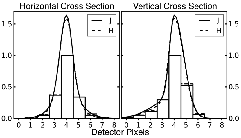
Figure 3: Orthogonal cross sections through the center of the IFU PSF fit for wavelengths 1.25 $\mu$m ($J$) and 1.58 $\mu$m ($H$). The curves illustrate the function given in Equation 2 with the parameters given in Table 1. The bars represent the same models after being downsampled to the detector resolution using the assumed intra-pixel response.

3.2 Spectrum Image Model

We built upon knowledge of the spectrograph PSF to characterize the coarse near-infrared spectra distributed across the IFU focal plane. Here we turned to our Moon and twilight sky calibration exposures, during which each microlens was illuminated with a strong, uniform, broad spectrum of light. An example image of this kind was illustrated in Figure 2. By isolating the small detector area containing an individual microlens signal, we can fit a set of parameters encoding the spectrum geometry.

Table 2: Definitions of parameters describing the geometry of an individual spectrum image. The mean, range, and standard deviation values of the parameters, as determined for the September 2009 focal plane, are also listed.

Parameter	Definition	Mean	Range	Std. Dev.
Position $\left(X_{0},Y_{0}\right)$	$\left(X_{1.37\mu\mbox{\tiny m}},Y_{1.37\mu\mbox{\tiny m}}\right)$	N/A	(0.0–2047.0, 0.0–2047.0)	N/A
Height ($h$)	$Y_{1.10\mu\mbox{\tiny m}}-Y_{1.76\mu\mbox{\tiny m}}$	23.9 pixels	23.5–24.7 pixels	0.2 pixels
Tilt ($t$)	$\left(X_{1.10\mu\mbox{\tiny m}}-X_{1.76\mu\mbox{\tiny m}}\right)/\left(Y_{1.10\mu\mbox{\tiny m}}-Y_{1.76\mu\mbox{\tiny m}}\right)$	0.044	0.0090–0.080	0.021

In Table 2 we have listed the parameters needed to describe the spectrum image of an individual microlens. The $\left(X_{0},Y_{0}\right)$ position coordinates are the most fundamental of these. They are referenced to the $\lambda$ = 1.37 $\mu$m point, which coincides with the sharp (blue) edge of the telluric water absorption trough between the $J$ and $H$ bands. The $X,Y$ coordinates index the full detector array from an origin at the pixel in the lower left (SW) corner of the image; all integral values align with a pixel center. Using similar notation, we defined the spectrum height and tilt based on the relative positions of the $\lambda$ = 1.10 $\mu$m and 1.76 $\mu$m points, which roughly correspond to the edges of our passband. From the position, height, and tilt, the coordinates of an arbitrary wavelength in the spectrum can be calculated by the following parametrized equations:

$$\begin{array}[]{lr}X(w)=X_{0}+th\left(\frac{9-w}{22}\right)\\ Y(w)=Y_{0}+h\left(\frac{9-w}{22}\right)\end{array}$$ (4)

where $h$ is height, $t$ is tilt, and $w=\left(\lambda-1.1\>\mu\mbox{m}\right)/0.03\>\mu$m. By this definition, each integral step in $w$ corresponds to 0.03 $\mu$m, so there is a total of 22 such increments from 1.10 $\mu$m and 1.76 $\mu$m. Using the same wavelength parameter, we can specify the intrinsic spectrum incident on the focal plane by some function $s(w)$ for $0\leq w\leq 22$.

We introduce the concept of spectrum trace to model the layout of the spectrum by an ideal “skeleton” image formed by a train of impulse functions, unencumbered by diffraction and focus effects. The trace is discretized in the same manner as the PSF model, at a resolution $M$ times higher than that of the detector. In this case, however, we use a lower spatial sampling rate factor of $M=7$ to balance reasonable execution speed and performance. By convolving the trace with the reverse of the PSF (rotated 180^∘), and downsampling the result, we can synthesize a spectrum image as measured by the detector (Figure 4). The position, height, and tilt parameters, along with the intrinsic spectrum can then be adjusted by a least squares fitting algorithm until the downsampled result matches the data cutout.

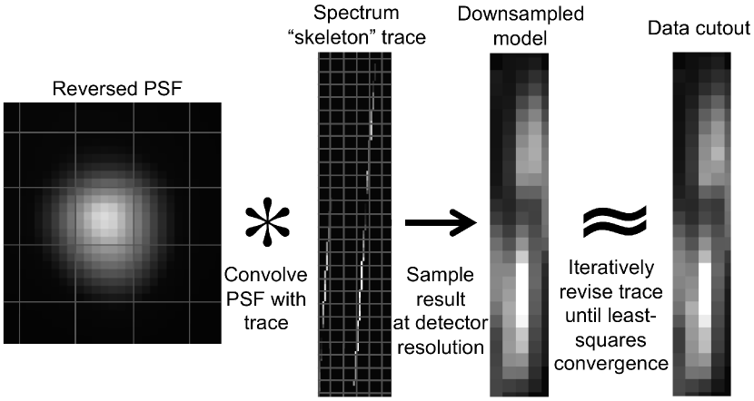
Figure 4: Diagram summarizing the microlens spectrum modeling procedure. On the far left, the IFU PSF model (reflected about the center) is shown with a spatial sampling factor 7 times that of the detector, with an overlaid grid of gray lines representing pixel boundaries. We convolve this with the spectrum model trace shown in the next panel (again shown with a gray grid to illustrate the scale of detector pixels) in order to simulate the true light distribution. To test the accuracy of the trace, we downsample the convolution result to the detector resolution, and compare it to the data cutout being fit. The fitting algorithm switches between adjusting the trace parameters and repeating the convolution and downsampling procedure until the model converges.

A cutout spanning an area of $9\times 29$ detector pixels is sufficient to enclose an individual spectrum as well as major portions of the two nearest neighbors. At the start of the fitting procedure, the cutout is aligned such that the ($X_{0},Y_{0}$) reference point of the spectrum nearly corresponds to pixel position (4, 16) in the detector-downsampled trace array. Two free parameters in the model, $\Delta X$ and $\Delta Y$, allow the algorithm to refine the initial position guess alongside the other geometrical properties. For a given microlens spectrum, the following equations define the conversion between $X,Y$ detector indices and $u,v$ trace array indices:

$$\begin{array}[]{lr}u=\left(X-X_{0}+\frac{9}{2}+\Delta X\right)M\\ v=\left(Y-Y_{0}+\frac{33}{2}+\Delta Y\right)M\\ \end{array}$$ (5)

from which it follows that the trace indices of the 1.37 $\mu$m reference point are $\left(u_{0},v_{0}\right)=\\ \left(M\left(\frac{9}{2}+\Delta X\right),M\left(\frac{33}{2}+\Delta Y\right)\right)$. Based on the typical interval between spectra along a microlens, we set the 1.37 $\mu$m reference points of the neighboring spectra by $(u_{0\uparrow},v_{0\uparrow})=(u_{0}+3.3M,v_{0}+10.0M)$ and $(u_{0\downarrow},v_{0\downarrow})=(u_{0}-3.3M,v_{0}-10.0M)$.

The trace signal is dispersed over the same line segment defined in Equation set 4, with intrinsic spectrum function $s(w)$. The neighboring spectra are parametrized by the same shape with respect to their own reference points, ($u_{0\uparrow},v_{0\uparrow}$) and ($u_{0\downarrow},v_{0\downarrow}$). We form separate trace arrays for the $J$- and $H$-band halves of the spectra, designated $\mathcal{T}_{J,M}(u,v)$ and $\mathcal{T}_{H,M}(u,v)$. We do this in anticipation of separate convolution operations with the $J$- and $H$-band PSFs (Figure 3). The two respective trace arrays are defined as follows:

$$\begin{array}[]{lr}\mathcal{T}_{J,M}(u,v)=\left\{\begin{array}[]{ll}s(w)&-\frac{1}{2}<u-u_{0}-t(v-v_{0})\leq\frac{1}{2}\;\;\;\mbox{and}\;\;\;0\leq w<10\\ s(w_{\uparrow})&-\frac{1}{2}<u-u_{0\uparrow}-t(v-v_{0\uparrow})\leq\frac{1}{2}\;\;\;\mbox{and}\;\;\;0\leq w_{\uparrow}<10\\ s(w_{\downarrow})&-\frac{1}{2}<u-u_{0\downarrow}-t(v-v_{0\downarrow})\leq\frac{1}{2}\;\;\;\mbox{and}\;\;\;0\leq w_{\downarrow}<10\\ 0&\mbox{otherwise}\\ \end{array}\right.\\ \mathcal{T}_{H,M}(u,v)=\left\{\begin{array}[]{ll}s(w)&-\frac{1}{2}<u-u_{0}-t(v-v_{0})\leq\frac{1}{2}\;\;\;\mbox{and}\;\;\;10\leq w\leq 22\\ s(w_{\uparrow})&-\frac{1}{2}<u-u_{0\uparrow}-t(v-v_{0\uparrow})\leq\frac{1}{2}\;\;\;\mbox{and}\;\;\;10\leq w_{\uparrow}\leq 22\\ s(w_{\downarrow})&-\frac{1}{2}<u-u_{0\downarrow}-t(v-v_{0\downarrow})\leq\frac{1}{2}\;\;\;\mbox{and}\;\;\;10\leq w_{\downarrow}\leq 22\\ 0&\mbox{otherwise}\end{array}\right.\\ \end{array}$$ (6)

where $w=9-\frac{22}{Mh}\left(v-v_{0}\right)$, $w_{\uparrow}=9-\frac{22}{Mh}\left(v-v_{0\uparrow}\right)$, and $w_{\downarrow}=9-\frac{22}{Mh}\left(v-v_{0\downarrow}\right)$.

To test a given set of spectrum model parameters, we convolve the $J$ and $H$ trace arrays with the reverse of the PSF model (such that $\mathcal{P}^{\prime}_{M}(i,j)=\mathcal{P}_{M}(-i,-j)$), giving a high-resolution model of the light distribution on the focal plane, $\mathcal{S}_{M}(u,v)$:

$$\mathcal{S}_{M}=\mathcal{T}_{J,M}*\mathcal{P}^{\prime}_{J,M}+\mathcal{T}_{H,M}*\mathcal{P}^{\prime}_{H,M}$$ (7)

Implicitly, we have zero-padded the trace arrays before the convolution, and trimmed the result to the original $9M\times 29M$ array size. The detector-downsampling operation is similar to that used earlier for the PSF model:

$$\mathbb{S}(x,y)=b+\sum_{i=0}^{M-1}\sum_{j=0}^{M-1}\mathcal{S}_{M}(i+Mx,j+My)\mathcal{R}_{M}(i,j)$$ (8)

However, one new variable has been introduced in Equation 8: $b$, a constant offset added to each pixel in the downsampled image model. This is one more parameter open to adjustment by the fitting procedure, which takes into account any background level of scattered light present in the data cutout. For a point source, in some focal plane locations this background reaches up to 3% of the 99.5 percentile-level count rate, considering all detector pixels. Therefore, it becomes especially significant for an exposure of a source as bright as the Moon. The resulting synthetic spectrum image $\mathbb{S}$ can be directly compared with the data cutout (Figure 4). In principle, the least squares fitting algorithm (the MPFIT program in our case) converges on the data cutout over many loops, switching between revising the trace model parameters and comparing the downsampled result to the data.

The combination of unknown position, shape, and intrinsic spectrum $s(w)$ presents too many free parameters for a fitting algorithm to accurately solve for at once. In practice, we need to iteratively build up constraints, starting from as few assumptions as possible. One aspect of the Moon/sky calibration exposure we can take advantage of is the fact that the intrinsic spectrum, $s(w)$, is identical across the image, apart from scale factors due to large-scale variations in sensitivity over the field of view. In addition, by referring to the laser calibration images, we can make very good initial guesses of the height and tilt for a given region of the focal plane. Still, we found these constraints alone were insufficient to reach consistent solutions. The exact vertical position of the spectrum (encoded by $\Delta Y$ in Equation Set 5) proved especially difficult to determine with only limited information about the light source and the instrument response. To get over this barrier, we chose to use prior knowledge of the atmosphere’s transmission function—in particular, the shape imposed on the spectrum by the deep water absorption trough in the middle of the P1640 passband.

Figure 5 shows the expected transmission function of the atmosphere from 1.28 $\mu$m to 1.52 $\mu$m. The data points are based on the measurements made by Manduca & Bell (1979) from Kitt Peak (at altitude 6875 ft, comparable to the 5618 ft altitude of the Palomar Observatory Hale Telescope), here averaged over 0.01 $\mu$m bins. Instead of allowing the points inside the water trough ($6<w<14$) to vary freely, we impose the condition

$$s(w)=\left\{\begin{array}[]{ll}T_{\mbox{\tiny atm}}(w)s(6)&6<w<10\\ T_{\mbox{\tiny atm}}(w)s(14)&10\leq w<14\\ \end{array}\right.$$ (9)

where $T_{\mbox{\tiny atm}}(w)$ is the peak-normalized atmospheric transmission function plotted in Figure 5. Inside the water trough, $s(w)$ is discretized in 0.01 $\mu$m bins; outside, in 0.03 $\mu$m bins (integral values of $w$). Once the above assertion is in place, the fitting algorithm could at last reliably determine both the position and shape of the spectrum, as achieved in the example shown in Figure 4.

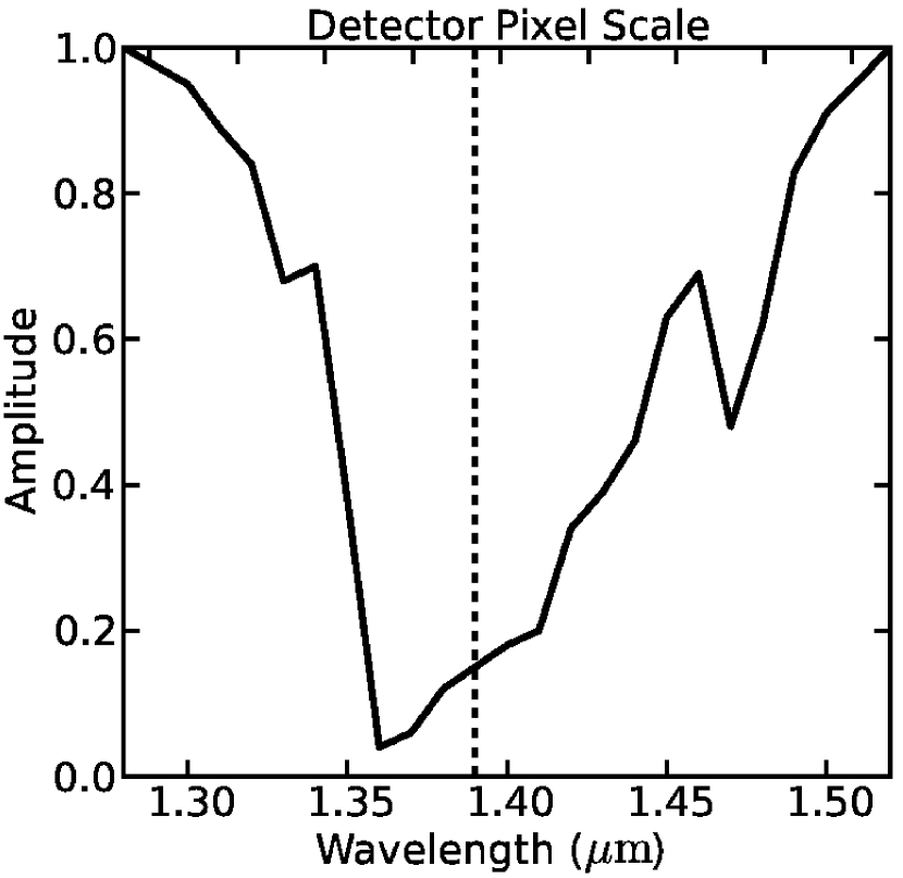
Figure 5: The atmospheric transmission function around the water absorption trough between the $J$ and $H$ bands, binned to 0.01 $\mu$m resolution, based on the measurements by Manduca & Bell (1979). The tick marks on the top axis indicate the scale of vertical detector pixels along the dispersion axis of the spectrum. During the spectrum fitting procedure, when the exact position and shape have not yet been established, the model trace spectrum $s(w)$ is forced to follow this profile in the range $\lambda=\mbox{1.30--1.50}\>\mu\mbox{m}$. The dotted line separates those points of $s(w)$ that are fixed relative to the free spectrum value at $\lambda=1.28\>\mu$m ($6<w<10$) versus $\lambda=1.52\>\mu$m ($10\leq w<14$).

3.3 Global Spectrograph Focal Plane Solution

We repeated the spectrum fitting procedure across the entire spectrograph image to form a global solution unique to the specific epoch of the Moon/sky calibration exposure. To minimize the number of free parameters before executing this, we first determined a mean intrinsic spectrum $\bar{s}(w)$ based on average of the $s(w)$ fit results from a sub-area of about 100 spectra near the center of the field of view. With the spectrum shape fixed, however, there needs to be a parameter that captures variations in overall signal strength across the focal plane. We designated an amplitude parameter $a$ to acts as a multiplicative constant, applied to $\bar{s}(w)$, and freely adjusted alongside $X_{0}$, $Y_{0}$, $h$, $t$, and $d$.

In Figure 6 we have displayed maps of the height, tilt, and amplitude parameters for one epoch. These maps proved essential to the challenging process of debugging the fitting routines. They also enable easy visual comparisons between focal plane properties at different times, and can serve as diagnostic tools during periods of modifications and upgrades to instrument optics. The maps in Figure 6 appear as rotated squares because the microlens array is by design rotated with respect to the detector (as shown previously in Figure 2). We index the microlenses using Cartesian coordinates $i$ and $j$ relative to an origin at the lower left corner. With these coordinates, a range of $0\leq i,j<250$ is sufficient to enclose the $3.8\times 10^{4}$ microlens spectra on the detector.

The ability to analyze the spatial distribution of the IFU spectra is also of great interest. A vector field, like those depicted in Figure 7, is an effective way to illustrate the evolution of the global spectrograph focal plane geometry. To make these plots, we first partitioned the calibration image into an array of $8\times 8$ boxes, each of width 256 detector pixels. For any two comparison epochs, each with spectrum position arrays $X_{0}(i,j)$ and $Y_{0}(i,j)$, we calculated the median of the differences $\Delta X_{0}(i,j)$ and $\Delta Y_{0}(i,j)$ inside each box, resulting in an $8\times 8$ array of vectors. Before plotting those vectors, we subtracted the median difference vector at the image center. In this way, we removed the effect of a trivial bulk shift between the focal plane patterns.

Depending on the duration of time between the pair of calibration images under consideration, the quivers representing the vectors need to be scaled up by different factors to reveal the subtle evolution. Once this is done, it becomes clear that the overall scale and orientation of the spectrograph focal plane pattern vary with time. More complicated, non-uniform distortions also play a role. In all cases, the magnitude of these changes are small enough that they would never be obvious from a mere “blinking” comparison of the source images. For example, the transformation from March 2009 to June 2009 can mostly be attributed to a rotation of the microlens array with respect to the detector (or vice versa) by an angle of merely $14^{\prime\prime}$. Likewise, between 28 June 2009 and 29 June 2009, the focal plane was magnified by about 0.003%. It is a fair guess that the changes we observe in global focal plane geometry are due to minute variations of environmental conditions inside the IFU dewar. However, it remains unclear what the relative contributions are from the various optics and the mechanical support structures. To an extent, the origin of these changes is not an issue, so long as each science data set can be attached to a solution that accurately reflects its particular geometry.

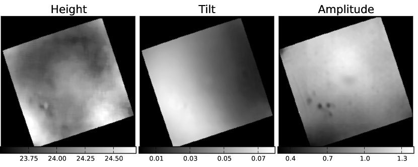
Figure 6: Maps of spectrum parameters making up one global spectrograph focal plane solution. This particular solution is based on the fit to the Moon calibration image acquired on 28 June 2009. The maps appear rotated due to the orientation of the microlens array with respect to the detector (see Figure 2). Height is shown in units of detector pixels, tilt is an inverse slope (unitless), and amplitude is mean-normalized.

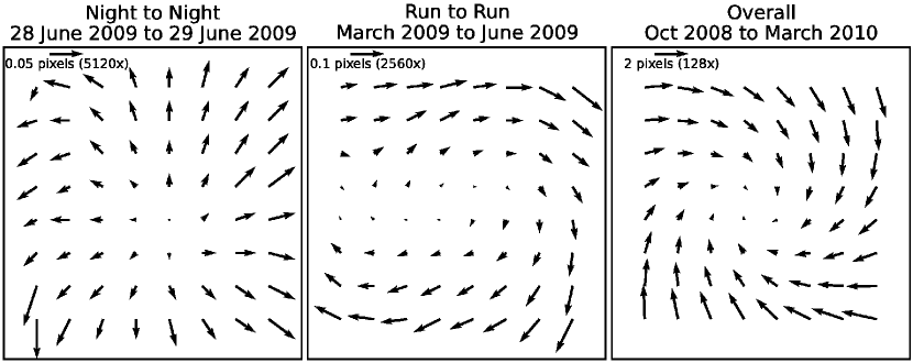
Figure 7: Vector field plots illustrating examples of the evolution of the spectrograph focal plane geometry over three time intervals: 1 day, 3 months, and 17 months. Each quiver represents the median change in spectrum position inside a box $1/8^{\mbox{\footnotesize th}}$ of the full image width. In the top left corner of each plot, a small legend indicates the relative scale of the quiver in terms of detector pixel widths. For each comparison, we customized the quiver scale factor to clearly reveal the transformation.

Another important product of our global fitting procedure is a synthetic image of the entire spectrograph focal plane. Using the established geometric parameters, we can inject an arbitrary source spectrum $s_{\star}(w)$ to simulate the distribution of light incident on the detector. The synthetic focal plane image is useful for inspecting the results of the global fit, and is also an essential ingredient in the algorithm used by the cube extraction pipeline to register the spectrograph image of an individual science exposure at sub-pixel precision (described in § 4.1.5). The formalism is analogous to that described for the individual spectrum cutout model in Equations 5–8. We designate $\mathcal{F}_{J}(p,q)$ and $\mathcal{F}_{H}(p,q)$ to represent the $J$- and $H$-band model trace arrays of the full spectrograph focal plane image, discretized at a spatial sampling rate $M$ times that of the detector. Since the HAWAII-2 detector array size is $2048\times 2048$, the trace arrays are defined over $p,q\in\{0,1,\dotsc,2048M-1\}$. Here we again settled on a sampling factor of $M$ = 7. Since as before, we require $M$ to be an odd integer $\geq 3$, there is always a pair of trace array indices $p,q$ aligned with the center of a given detector pixel $X,Y$:

$$\begin{array}[]{lr}p=MX+\frac{M-1}{2}\\ q=MY+\frac{M-1}{2}.\\ \end{array}$$ (10)

The trace array is determined by the position, height, and tilt solutions, now indexed by microlens coordinates $i,j$:

$$\begin{array}[]{lr}\mathcal{F}_{J,M}(p,q)={\displaystyle\sum\limits_{i=0}^{249}\sum\limits_{j=0}^{249}\mathcal{S}_{J,M,i,j}(p,q)}\\ \mathcal{F}_{H,M}(p,q)={\displaystyle\sum\limits_{i=0}^{249}\sum\limits_{j=0}^{249}\mathcal{S}_{H,M,i,j}(p,q)}\\ \end{array}$$ (11)

$$\begin{array}[]{l}\mbox{where}\\ \begin{array}[]{lr}\mathcal{S}_{J,M,i,j}(p,q)=\left\{\begin{array}[]{ll}s_{\star}(w_{ij})&-\frac{1}{2}<p-p_{0_{ij}}-t_{ij}(q-q_{0_{ij}})\leq\frac{1}{2}\;\;\;\mbox{and}\;\;\;0\leq w_{ij}<10\\ 0&\mbox{otherwise}\\ \end{array}\right.\\ \mathcal{S}_{H,M,i,j}(u,v)=\left\{\begin{array}[]{ll}s_{\star}(w_{ij})&-\frac{1}{2}<p-p_{0_{ij}}-t_{ij}(q-q_{0_{ij}})\leq\frac{1}{2}\;\;\;\mbox{and}\;\;\;10\leq w_{ij}\leq 22\\ 0&\mbox{otherwise}\end{array}\right.\\ \end{array}\\ p_{0_{ij}}=MX_{0_{ij}}+\frac{M-1}{2},\quad q_{0_{ij}}=MY_{0_{ij}}+\frac{M-1}{2},\quad\mbox{and}\>w_{ij}=9-\frac{22}{Mh_{ij}}\left(q-q_{0_{ij}}\right).\\ \end{array}$$ (12)

From the trace arrays, we obtain the spectrograph focal plane image model $\mathcal{I}_{M}(p,q)$ in the same manner as in § 3.2, by convolving them with their corresponding reversed PSF models:

$$\mathcal{I}_{M}=\mathcal{F}_{J,M}*\mathcal{P}^{\prime}_{J,M}+\mathcal{F}_{H,M}*\mathcal{P}^{\prime}_{H,M}$$ (13)

We implement these convolution operations in the Fourier domain to save computational time, which is otherwise a nuisance for the large dimensions of our arrays (Bracewell, 2006, chap. 6). With a spatial sampling factor of $M=7$, we obtain a factor of $\sim$ 50 using FFT-based convolution over direct convolution. In our experience, this cuts the execution time needed to form the synthetic image down from a few hours to a few minutes (assuming the global solution is already done).

Finally, we can obtain the detector-downsampled synthetic focal plane image, $\mathbb{I}(X,Y)$, by binning $\mathcal{I}_{M}$ to the detector resolution using the assumed intra-pixel response:

$$\mathbb{I}(X,Y)=\sum_{i=0}^{M-1}\sum_{j=0}^{M-1}\mathcal{I}_{M}(i+MX,j+MY)\mathcal{R}_{M}(i,j)$$ (14)

Note that this synthetic detector image is idealized in the sense that we have left out the amplitude modulations across the image ($a_{ij}$) as well as background light parameters ($d_{ij}$). For the purpose of registering a science spectrograph image, this is preferred, since we are only concerned with matching the shapes and positions of the spectra.

4 Data Cube Extraction Pipeline

The Project 1640 Data Cube Extraction Pipeline (PCXP), written in the GNU C programming language, automates the processing of raw P1640 detector images and their translation to reduced data cubes. A block diagram summarizing the steps applied to each image is shown in Figure 8. By design, the program is fast enough to use while observing, so that newly acquired images can be inspected in real time to monitor instrument performance and check for unknown objects. The data pipeline can also be used to process an arbitrarily large set of raw data at a later date. For post-processing, we feed the output of the PCXP into the Project 1640 Speckle Suppression Pipeline (PSSP), described by Crepp et al. (2011).

Two outer loops comprise the PCXP execution. First, the program steps through the detector data in the input directory specified by the user at the start time, processing each non-destructive read (NDR) sequence to form a reduced, registered spectrograph image. The second stage of the pipeline loops through the finished spectrograph images and extracts data cubes from each of them. Throughout these steps, the pipeline relies on the empirical model of the spectrograph focal plane described in § 3.

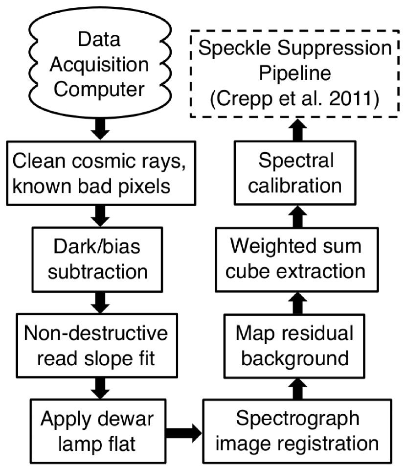
Figure 8: Block diagram of the Project 1640 Data Cube Extraction Pipeline (PCXP). Raw detector data are processed into reduced, registered spectrograph images (§ 4.1). In the second main loop, beginning with the residual background mapping, the spectrograph images are translated to data cubes with the help of the global spectrograph focal plane solution (§ 4.2).

4.1 Detector Image Processing

4.1.1 Cosmic Ray Removal

The pipeline identifies pixels contaminated by cosmic rays by checking for anomalous jumps in digitized count values within the NDR sequence. For each detector pixel, our algorithm determines the median increase in counts between successive reads over the course of the exposure. A count increment greater than five times the median is flagged as a cosmic ray event. At each pixel meeting this criterion, the count contribution of the cosmic ray event is subtracted from the read corresponding to the event as well as all the following reads, canceling out its influence. We chose our threshold based on inspections of images of faint occulted stars, with relatively noisy slopes. We blinked “before” and ”after” images to check that all apparent cosmic ray events, and no starlight-dominated pixels were erroneously flagged.

This method of cosmic ray removal only works for exposures consisting of more than two reads. For a shorter exposure there is no way to take advantage of the NDR detector mode to identify cosmic rays. In this case the pipeline passes the detector image through the IRAF NOAO cosmic ray cleaning algorithm.

4.1.2 Bias/Dark Subtraction

During each observing run, a set of “dark” NDR sequences are obtained by taking calibration exposures with the IFU in a cryogenic state identical to the scientific data acquisition mode, except that the coronagraph beam entrance window is capped to obstruct external light. These dark exposures record the bias, thermal, dark current, and badly-behaved “hot” pixel count values of the detector array at each read interval. The median of 11 dark NDR sequences for each exposure time is added to a permanent library directory of dark exposures, marked by date and exposure time. See Figure 9 for an example of a dark exposure. After loading the dat file of a science target, the first processing step of the pipeline is to find the most appropriate dark NDR sequence and perform a readwise subtraction.

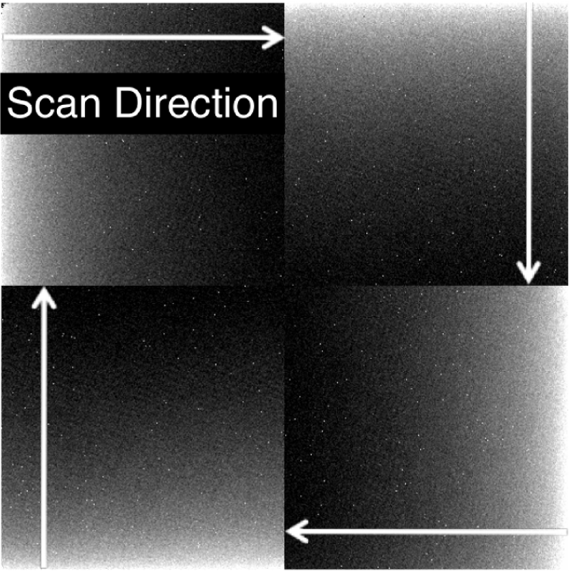
Figure 9: An example of a dark exposure used to subtract the bias, thermal counts, and hot pixels from science images. The “bias tilt”—the gradient in the bias pedestal—is strongest along the scan direction of each detector quadrant (each with its own read-out amplifier).

4.1.3 Non-destructive Read Slope Fitting

After subtracting the bias/dark component and removing the cosmic rays, the pipeline fits a slope to the ADU count versus time values recorded in the NDR sequence. This reduces the detector data for a given exposure to a single $2048\times 2048$ pixel representation of the spectrograph image. We employ an ordinary least-squares linear regression to determine the count rate for each pixel, eventually storing the floating point values in a FITS file in units of counts/second.

The slope fitting is complicated by pixel saturation caused by bright sources. However, the NDR detector mode is advantageous for handling this. In the case where a pixel reaches saturation at some point after the first two reads, the affected reads are simply excluded from that pixel’s linear regression. This approach, recommended after tests described by Ives (2008), extends the effective dynamic range of a long exposure by a factor of $\sim N_{reads}/2$. For pixels that reach saturation before the second read, a slope computation is not possible. If this saturation occurred between the first and second reads, then the slope can at least be approximated based on the difference between the first read value and an assumed zero level from the dark NDR sequence. However, in the case of a pixels saturating before the first read, this result will not be physically meaningful. To prevent erroneous measurements from being made by investigators analyzing images affected by saturation, the pipeline sets an appropriate header variable in the reduced FITS files. This header keyword indicates whether any of the detector pixels saturated, and if so, whether that occurred at the first, the second, or a subsequent read.

4.1.4 Detector Flat-Fielding

A externally controlled lamp inside the dewar of the P1640 IFU can fully illuminate the detector. To counteract pixel-to-pixel variations in detector sensitivity, we constructed a detector flat field map based on the mean of 12 dewar lamp exposures. Since the lamp intensity is not uniform across the detector, we used IRAF to fit a cubic spline surface to the normalized, mean dewar lamp image. We divided by the resulting spline surface to form the final detector flat, with large-scale variations removed (see the next section for an explantation of how large-scale variations in sensitivity are corrected for during cube extraction). The standard deviation of pixel values in the detector flat field map is 0.13. After the NDR slope-fitting step, the pipeline divides the spectrograph image by the flat field map to compensate for pixel-to-pixel variations. For locations in the flat field map with exceptionally low values ($<0.3$), no division is carried out since doing so would tend to enhance the noise induced by weak, problematic pixels.

4.1.5 Spectrograph Image Registration

Due to flexure—varying mechanical stress on the instrument while the telescope slews—the projection of the microlens array onto the detector changes over the course of an observing period. The plot in Figure 10 illustrates the magnitude of this effect based on measurements from three observing runs. Between targets, the positions of the spectra on the detector can uniformly shift by up to 2 pixels in each direction. Between observing runs there is a more pronounced, systematic shift in the spectrograph-detector alignment. To accurately extract the data, the pipeline needs to register the precise offset between each spectrograph image and the focal plane model of the corresponding epoch. We accomplish this through two stages: first a crude estimate based on a cross-correlation with the downsampled spectrograph image model (array $\mathbb{I}$ in Equation 14), followed by a more elaborate approach to refine the offset to sub-pixel precision.

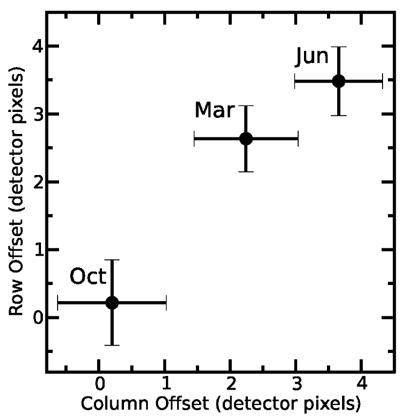
Figure 10: Example distributions of the spectrograph-detector alignment offsets with respect to a canonical template. The mean offsets, with bars indicating the standard deviations in each direction, are plotted for three P1640 observing runs: October 2008, March 2009, and June 2009.

For efficiency, the initial cross-correlation is restricted to a $200\times 200$ square pixel section of the science image $\mathbb{D}(X,Y)$. We denote this cutout box with a tilde accent on top of the original array symbol:

$$\tilde{\mathbb{D}}(x,y)=\mathbb{D}\left(X_{p}-100+x,Y_{p}-100+y\right)\quad\mbox{for}\;0\leq x,y<200.$$ (15)

Likewise we use $\tilde{\mathbb{I}}$ to represent the same section from the downsampled focal plane image model. The center of the box, $(X_{p},Y_{p})$, is chosen based on the average count rate computed within $16\times 16$ partitions across the image, so as to enclose spectra with relatively high signal strength. In a typical science image with the star occulted by the coronagraph, this is near the center of the image, where the residual starlight is brightest.

We cross-correlate $\tilde{\mathbb{I}}$ and $\tilde{\mathbb{D}}$ to determine the crude offset. A given science focal plane pattern is not expected to stray more than two pixels away from the calibration exposure of the matching epoch. Furthermore, the periodicity of the spectrum pattern ensures that large lags will merely introduce degenerate solutions. Therefore, we do not compute the full two-dimensional cross-correlation array, but merely a small region bounded by horizontal and vertical lags up to 4 pixels in each direction:

$$\tilde{\mathbb{C}}_{0}(r,s)={\displaystyle\sum\limits_{x=4}^{195}\sum\limits_{y=4}^{195}}\tilde{\mathbb{I}}(x-r,y-s)\tilde{\mathbb{D}}(x,y)\quad\mbox{for}\>-4\leq r,s\leq 4$$ (16)

The summation limits take the lag range into account in order to avoid the influence of non-overlapping array edges. The lag combination that maximizes $\tilde{\mathbb{C}}(r,s)$, which we denote $(r_{p},s_{p})$, is our initial guess for the horizontal and vertical displacement of $\mathbb{D}$ with respect to $\mathbb{I}$.

The second stage of the registration routine determines separately the fine $X$ and $Y$ offsets. As apparent in Figure 2, the spectral dispersion is almost completely aligned with the $Y$ axis of our detector image coordinate system. As a consequence, the shape of a spectrum’s horizontal cross-section at a given wavelength is determined much more by the spectrograph PSF shape than by the intrinsic spectrum of the light source. It is effectively the cross-dispersion profile commonly referred to in literature on more conventional spectroscopic observations (e.g, Miskey & Bruhweiler, 2003). Therefore, to measure the effect of a slight horizontal offset on the detector-sampled image, we can start with the high-resolution model of the light distribution $\mathcal{I}_{M}$ (Equation 13 from § 3.3), even though its intrinsic spectrum does not necessarily match the data. To simulate how the detector would “see” the image model for a range of small fractional-pixel offsets from the initial alignment, we downsample $\mathcal{I}_{M}$ as in Equation 14, but with the detector sampling array shifted by a range of horizontal sub-pixel offsets indexed by the variable integer $\delta$:

$$\begin{array}[]{lr}\tilde{\mathbb{I}}_{\delta}(x,y)={\displaystyle\sum\limits_{i=0}^{M-1}\sum\limits_{j=0}^{M-1}\mathcal{I}_{M}(M(X_{p}-100+x)+i-\delta,M(Y_{p}-100+y)+j)\mathcal{R}_{M}(i,j)}\\ {\displaystyle\mbox{for}\quad 0\leq x,y<200\quad\mbox{and}\;-\frac{M-1}{2}\leq\delta\leq\frac{M-1}{2}.}\\ \end{array}$$ (17)

Now we reevaluate the cross-correlation peak for the $M$ fine horizontal offsets values, with $r$ and $s$ fixed at $r_{p}$ and $s_{p}$:

$$\tilde{\mathbb{C}}_{\delta}(r_{p},r_{s})={\displaystyle\sum\limits_{x=4}^{195}\sum\limits_{y=4}^{195}}\tilde{\mathbb{I}}_{\delta}(x-r_{p},y-s_{p})\tilde{\mathbb{D}}(x,y)\quad\mbox{for}\;-\frac{M-1}{2}\leq\delta\leq\frac{M-1}{2}.$$ (18)

The fractional offset index $\delta$ that maximizes $\tilde{\mathbb{C}}_{\delta}(r_{p},r_{s})$ gives the fine horizontal displacement of the data, $\delta$, with respect to the crude initial guess, $r_{p}$. The full horizontal offset is $r_{p}+\delta/M$ detector pixel widths.

We originally intended to use the same approach to determine the fine vertical offset. Unfortunately, in this case the disparity between the intrinsic spectrum of the data and the image model strongly biases the cross-correlation result. In a typical science image, the cutout box $\tilde{\mathbb{D}}$ contains $\sim$10 speckles. Their chromatic position dependence (as illustrated in Figure 1) causes steep brightness gradients in the spectra formed on the spectrograph focal plane, since a given microlens will collect light from a speckle over only a fraction of the passband. Whatever intrinsic spectrum is built into the image model, $\mathcal{I}_{M}$, will significantly differ from that of most of the sample. We found that the effects of these disparities do not average out over an ensemble. Instead, they systematically push the cross-correlation result up or down by a degree that does not reflect the actual relative wavelength alignment.

Instead of using the image model as an alignment template, we return to the fitting approach described in § 3.2. This time, however, rather than fitting the full spectrum parameter set, we concentrate on the region with the most information about the vertical position: the telluric water absorption trough. Therefore, we confine the least-squares fit region to a $3\times 11$ box, aligned such that the 1.37 $\mu$m reference point is near the middle pixel on the 8th row.

We further simplify the spectrum fit by describing the local light source with merely two parameters: an amplitude and color. The other free parameters are the background light offset and the vertical position. The height and tilt are already known from the calibration image solution, and the horizontal position is fixed based on the previous step in the registration algorithm. As in Equation 9, the spectrum trace points with wavelengths $1.28\>\mu\mbox{m}<\lambda<1.52\>\mu$m are again tied to the transmission function plotted in Figure 5. The anchor points at $\lambda=$1.28 $\mu$m and 1.58 $\mu$m are set based on the amplitude and color parameters.

To get a diverse set of spectrum shapes spanning a wide region of the speckle halo, during the fine vertical offset fitting procedure we sample 121 spectra over a $600\times 600$ pixel box (as compared to the $200\times 200$ pixel box used for the horizontal registration). Of the 121 fits, the median vertical offset is taken as the final value, and rounded to the nearest 1/7th of a pixel to match the quantization of the fine horizontal offset. In trial runs, we found the vertical offsets determined from the full set of sample spectra follow a Gaussian distribution, with standard deviation 0.2–0.4 pixel widths, depending on the source image. We accept this as the uncertainty in the vertical registration.

4.2 Cube Extraction

4.2.1 The Role of the Global Spectrograph Focal Plane Solution

In order to form a data cube, the pipeline must “know” where individual spectra are positioned on the focal plane, and furthermore, which points of those spectra correspond to a given wavelength. We rely on the global spectrograph focal plane solution described in § 3.3 to establish the image geometry for each epoch under consideration. One of the products of the calibration image fitting procedure is a text file tabulating the positions of all $3.8\times 10^{4}$ spectra alongside their corresponding microlens indices. This table, combined with the results of the registration algorithm (§ 4.1.5) and the maps of height and tilt parameters give all the information needed to organize the detector data for a given science image.

The amplitude map produced during the global fit (see Figure 6) also has an important role. It compliments the dewar lamp flat described in § 4.1.4 by capturing the larger-scale variations in sensitivity across the field of view. By looking up the amplitude parameter associated with a given microlens, we can appropriately scale any detector samples from that spectrum to compensate for optical effects such as vignetting.

4.2.2 Residual Background Map

Despite the numerous stages in the detector image processing, some minor extraneous background structure persists into the processed focal plane image. This component, superimposed on the real signal, is caused by a combination of residual bias counts, scattered light within the instrument, and thermal contamination from outside the dewar (unaccounted for in the dark subtraction). In the cube extraction routine, after loading an individual focal plane image, the pipeline forms a map of background count rates based on measurements between spectra.

Figure 11 shows the regions used to estimate the background count rate associated with a given microlens. The upper left box is situated so that its bottom row is matched with the $\lambda=1.28\>\mu$m point (rounded to the nearest row), and the bottom row of the lower right box is on level with $\lambda=1.67\>\mu$m. For both background boxes, the near side is spaced three columns from the rounded center of the spectrum.

The pipeline takes the median of the sample of the pixels in both $2\times 5$ dark regions and stores this in a residual background map. After forming the background estimates for all microlenses, the resulting map is smoothed with a box median filter and stored for use in the inner extraction loop.

4.2.3 Weighted Sum Extraction

Our cube extraction method is summarized in Figure 11. After forming the background map, the extraction routine loops through microlens indices $i$ and $j$. For each microlens, we retrieve the parameters from the global spectrograph focal plane solution: position, height, tilt, and amplitude (represented by the variables $(X_{0_{ij}},Y_{0_{ij}})$, $h_{ij}$, $t_{ij}$, and $a_{ij}$, respectively). An inner loop steps through 23 wavelength channels in 0.03 $\mu$m increments between $\lambda=1.10\>\mu$m and 1.76 $\mu$m. We index these channels by integer values of $w$ ($0\leq w\leq 22$), and determine the extraction target point for each cube element, or spaxel, as follows (cf. Equation set 4):

$$\begin{array}[]{lr}X_{c_{ij}}(w)=X_{0_{ij}}+r_{p}+\delta/M+t_{ij}h_{ij}\left(\frac{9-w}{22}\right)\\ Y_{c_{ij}}(w)=Y_{0_{ij}}+s_{p}+\varepsilon/M+h_{ij}\left(\frac{9-w}{22}\right)\end{array}$$ (19)

where $r_{p}$ and $s_{p}$ are the crude horizontal and vertical offsets, and $\delta$ and $\epsilon$ are the fine horizontal and vertical offset indices determined by the registration algorithm (§ 4.1.5) for the current reduced spectrograph image, $\mathbb{D}(X,Y)$. We use a hat symbol to designate the same coordinates rounded to the nearest pixel center: $\left(\hat{X}_{c_{ij}}(w),\hat{Y}_{c_{ij}}(w)\right)$.

The spaxel for each microlens and wavelength combination is based on the weighted sum over a $3\times 3$ detector pixel square centered on $\left(\hat{X}_{c_{ij}}(w),\hat{Y}_{c_{ij}}(w)\right)$:

$$\mathcal{C}(i,j,w)={\displaystyle\sum\limits_{m=-1}^{1}\sum\limits_{n=-1}^{1}\mathbb{W}_{\alpha,\beta,w}(m,n)\left(\mathbb{D}\left(\hat{X}_{c_{ij}}(w)+m,\hat{Y}_{c_{ij}}(w)+n\right)-b_{ij}\right)/a_{ij}.}$$ (20)

The weights $\mathbb{W}_{\alpha,\beta,w}(m,n)$ applied to the detector samples are based on the PSF model, downsampled and truncated to the $3\times 3$ pixel extraction box as follows:

$$\mathbb{W}_{\alpha,\beta,w}(m,n)=\left\{\begin{array}[]{ll}{\displaystyle\Gamma_{J}(\alpha,\beta)\sum\limits_{i=0}^{M-1}\sum\limits_{j=0}^{M-1}\mathcal{P}_{J,M}\left(i+(m+4)M-\alpha,j+(n+4)M-\beta\right)\mathcal{R}_{M}(i,j)}\\ \quad\quad\mbox{if}\;\;0\leq w<10\\ \\ {\displaystyle\Gamma_{H}(\alpha,\beta)\sum\limits_{i=0}^{M-1}\sum\limits_{j=0}^{M-1}\mathcal{P}_{H,M}\left(i+(m+4)M-\alpha,j+(n+4)M-\beta\right)\mathcal{R}_{M}(i,j)}\\ \quad\quad\mbox{if}\;\;10\leq w\leq 22\\ \end{array}\right.,$$ (21)

defined for $-1\leq m,n\leq 1$. The formulas for the $J$- and $H$-band PSFs, $\mathcal{P}_{J,M}$ and $\mathcal{P}_{H,M}$, as well as the intra-pixel response, $\mathcal{R}_{M}$, can be found in § 3.1. The integers $\alpha$ and $\beta$ encode the offsets of the extraction target point from the extraction box center:

$$\begin{array}[]{lr}\alpha=\mathit{Round}\left(\left(X_{c_{ij}}(w)-\hat{X}_{c_{ij}}(w)\right)M\right)\\ \beta=\mathit{Round}\left(\left(Y_{c_{ij}}(w)-\hat{Y}_{c_{ij}}(w)\right)M\right).\\ \end{array}$$ (22)

The resulting indices take on integer values in the range $-\frac{M-1}{2}\leq\alpha,\beta\leq\frac{M-1}{2}$ (corresponding to offsets up to $\frac{3}{7}$ of a pixel width in each direction when $M=7$). Lastly, the $\Gamma$ factor in front of each weight formula compensates for the effect that the offset between the PSF center and the extraction box center has on the sum of products in Equation 20. The need for this can be qualitatively understood by the fact that the overall flux in a $3\times 3$ pixel sample of the PSF decreases when the peak is offset from the center. The $\Gamma$ correction factor varies from unity at perfect alignment up to 1.09 in the worst case for extreme offsets.

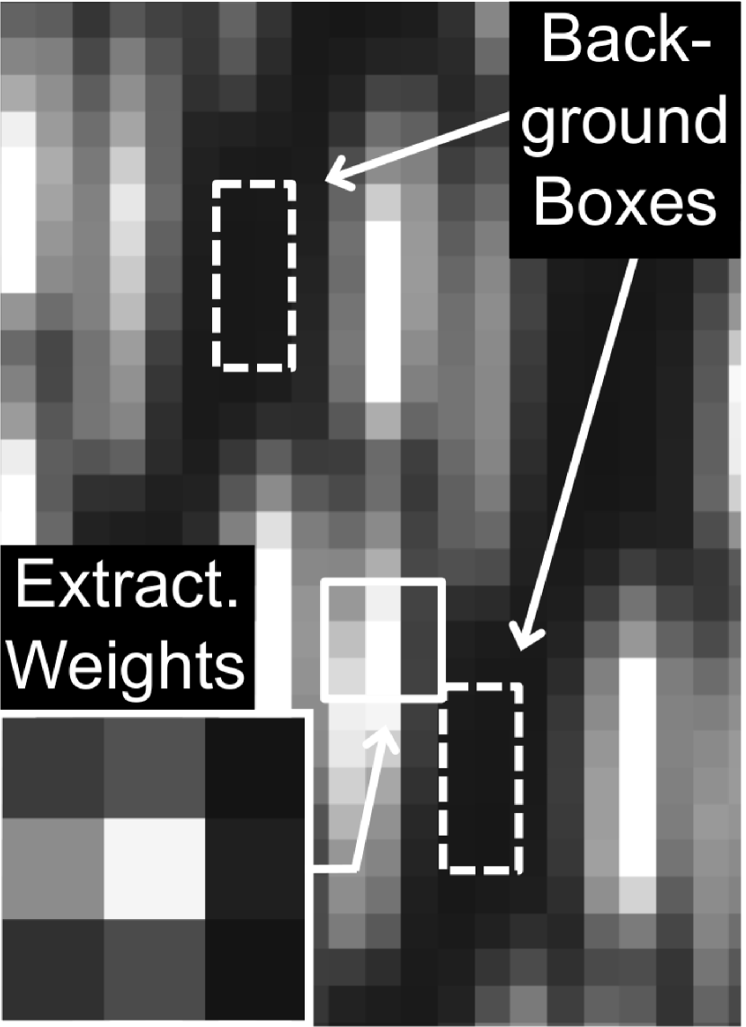
Figure 11: Diagram of the P1640 cube extraction method. We step down the spectrum in 0.03 $\mu$m increments, using the global focal plane solution to select a $3\times 3$ pixel region for each spaxel in the cube. The sum of the extracted samples is weighted based on the fractional offset of the true extraction target point from the box center. In the example shown here, the weighting scheme (bottom left inset) captures the leftward skew of the spectrum cross section at this particular wavelength. The two dashed boxes outline the “dark” regions used to sample the local background level around each spectrum.

4.2.4 Spectral Calibration

For a given microlens, the separation between the extraction target points of the first and last channels—corresponding to $\lambda=1.10\>\mu\mbox{m and }1.76\>\mu$m—is typically about 24 detector pixels. Since we use $3\times 3$ pixel boxes to extract a signal for each of 23 channels spanning that length, the footprints of adjacent channels necessarily overlap. We have examined the effect of this by extracting data cubes directly from the laser calibration images (discussed in § 3.1). From these cubes, we compared the mean flux in neighboring cube channels. The results, plotted in Figure 12 for 1.25 $\mu$m and 1.58 $\mu$m emission, reveal the effective filter shape of an individual data cube channel.

The cube channel filters exhibit a full width half-maximum value of $\sim$ 70 nm at both $J$ and $H$ band. Knowledge of this profile is essential for comparisons between P1640 data and existing astronomical spectra. We cannot simply bin a reference spectrum to the channel spacing; we must also convolve it with the cube channel filter before comparing it to data cube measurements. Suppose an object appears in a data cube, and we carry out channel-wise photometry to find a spectrum $\mathcal{A}(w)$, $0\leq w\leq 22$. To compare this meaningfully to an established spectrum, $\mathcal{B}(\lambda)$, acquired by some other instrument with wavelength bin width $\Delta\lambda$, requires two steps. First, we re-bin $\mathcal{B}(\lambda)$ to the cube channel interval, 0.03 $\mu$m, to form an intermediate-resolution spectrum $\mathcal{B}^{\prime}(w)$:

$$\mathcal{B}^{\prime}(w)=\left\{\begin{array}[]{cr}{\displaystyle\sum\limits^{1.115+0.03w\>\mu\mbox{\scriptsize m}}_{\lambda=1.085+0.03w\>\mu\mbox{\scriptsize m}}\mathcal{B}(\lambda)\Delta\lambda}&\quad 0\leq w\leq 22\\ 0&\mbox{otherwise.}\end{array}\right.$$ (23)

We then convolve the intermediate-resolution spectrum $\mathcal{B}^{\prime}$ with the cube channel filters $\mathfrak{F}_{J}(z)$ and $\mathfrak{F}_{H}(z)$. The filter functions are defined to follow the profiles shown in Figure 12 for $-3\leq z\leq 3$ (so that $z=0$ corresponds to the central peak of the filter), and are zero-valued outside that range.

$$\mathcal{B}^{\prime\prime}(w)=\left\{\begin{array}[]{ll}{\displaystyle\frac{\sum\limits^{3}_{z=-3}\mathfrak{F}_{J}(z)}{\sum\limits^{3}_{z=-w}\mathfrak{F}_{J}(z)}\sum\limits^{3}_{z=-3}\mathcal{B}^{\prime}(w+z)\mathfrak{F}_{J}(z)}&0\leq w<10\\ {\displaystyle\frac{\sum\limits^{3}_{z=-3}\mathfrak{F}_{H}(z)}{\sum\limits^{22-w}_{z=-3}\mathfrak{F}_{H}(z)}\sum\limits^{3}_{z=-3}\mathcal{B}^{\prime}(w+z)\mathfrak{F}_{H}(z)}&10\leq w\leq 22\\ \end{array}\right.$$ (24)

The ratios in front of each convolution sum compensate for the effect of the spectrograph passband edges on the filtering (they are unity when $w$ is at least three channels from both passband edges). The resulting spectrum, $\mathcal{B}^{\prime\prime}(w)$, is smoothed to the same resolution as the cube-derived spectrum $\mathcal{A}(w)$. If $A(w)$ has been corrected for the P1640 spectral response, then the two spectra can be directly compared, apart from some scale factor. If on the other hand, $\mathcal{A}(w)$ is a “raw” cube spectrum, with undetermined spectral calibration, and $\mathcal{B}^{\prime\prime}(w)$ refers to the same source, then it can be used to correct $\mathcal{A}(w)$—and, in general, any P1640 data cube, as described next.

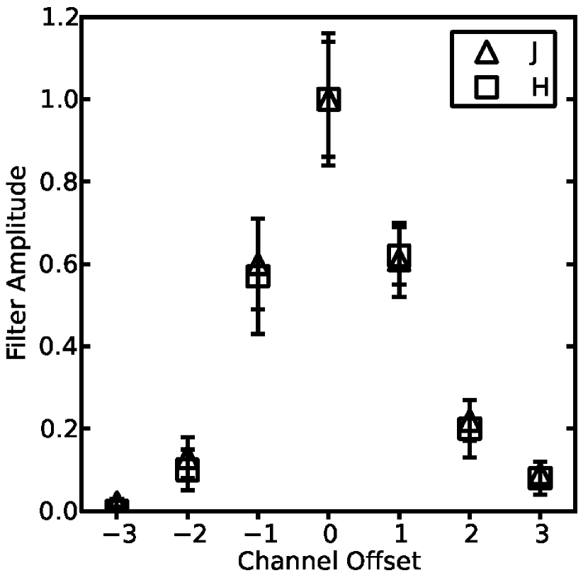
Figure 12: Normalized response of the P1640 cube extraction to 1.25 $\mu$m and 1.58 $\mu$m laser sources. These are the effective filter profiles assumed for cube channels in $J$ and $H$ band, respectively. The error bars indicate the standard deviation of the 100$\times$100 spaxel measurement sample.

We characterize the wavelength-dependent sensitivity of P1640, or spectral response function, by comparing the “raw” data cube count values of an unocculted reference star (observed off-axis from the coronagraph focal plane mask) with its established near-infrared spectrum. In practice, we have chosen stars with spectra archived in the NASA Infrared Telescope Facility (IRTF) Spectral Library to calibrate our response (Rayner et al., 2009). The spectral response function is determined by dividing the re-binned, smoothed reference spectrum ($\mathcal{B}^{\prime\prime}(w)$, in the notation above) by the spectrum of the same source derived from a P1640 data cube.

We measure the signal of the observed reference star by carrying out aperture photometry on each channel image making up the data cube, enclosing the third Airy ring. To capture the wavelength-dependent scaling of the coronagraph PSF, we linearly increased the photometric aperture radius from 13 to 20 spaxels across the passband. The resulting response curve for one calibration star, HD 75555 ($V=8.1$; spectral type F5.5III-IV), is shown in Figure 13. The response curve shows the expected roll-off at the edges of the operating range due to telluric water absorption features. The valley centered near $1.4~{}\mu$m is likewise due to water absorption between $J$ and $H$ band. The overall climb in the response towards longer wavelengths is caused by the wavelength-dependence of three effects in combination: the energy per photon as dictated by the Plank relation, $E=\frac{hc}{\lambda}$; detector quantum efficiency; and the transmission of the blocking filter at the IFU entrace.

We normalize the spectral response function to its mean value before storing it for general application to data cubes. The cube extraction pipeline loads one of these mean-normalized spectral response functions into memory before beginning the cube extraction routine. If the appropriate switch is set by the user, the pipeline will divide the spaxel values in each channel image by the corresponding response function value.

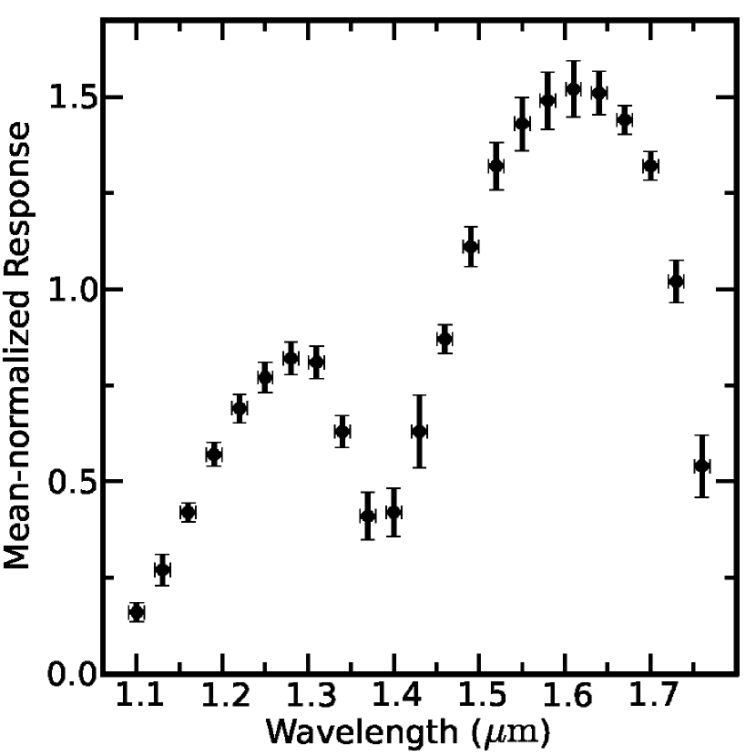
Figure 13: P1640 response curve, determined through a comparison between photometry on an unocculted star’s data cube (HD 75555, in this case) with the established spectrum of the star archived in the Infrared Telescope Facility Spectral Library.

4.2.5 Error Sources

Uncertainty in the global spectrograph focal plane solution, the image registration, and the weighting function combine to contribute a pseudo-random error to each cube point, at a level of $\sim$ 5% of the spaxel value. We extracted cubes from the Moon calibration images to estimate the magnitude of this error. Since spatial amplitude variations are compensated for during extraction, ideally any given spatial cross-section of a cube extracted from a calibration image would appear flat. Instead, we observe a standard deviation of 3%, with some variation between channels and areas of the image.

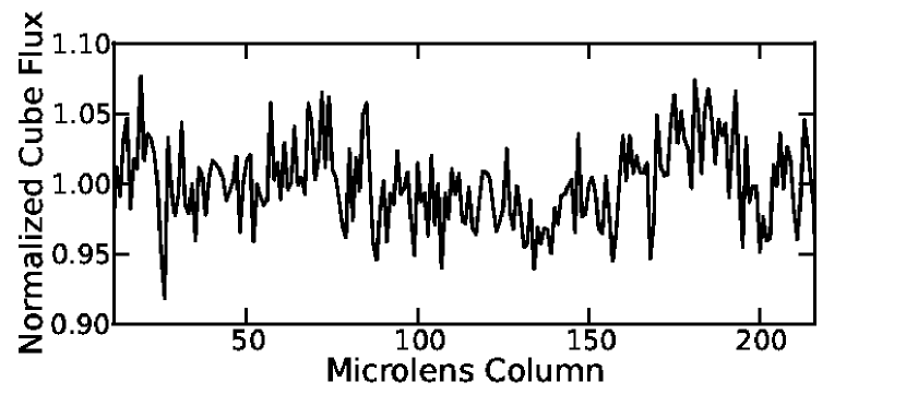
Figure 14: A row in a data cube extracted from a June 2009 Moon calibration image, with flux values normalized to unity. The scatter in flux across the row (here the standard deviation is 3%) reveals flux-proportional errors in the cube extraction.

There are also systematic errors caused by light from adjacent microlenses overlapping on the focal plane, which we refer to as cross-talk. The horizontal space between spectra on the focal plane is 3.3 detector pixels, and yet we know from the spectrograph PSF model (Figure 3) that about 10% of the downsampled PSF flux falls outside the central three columns. As a result, a small fraction of light from one microlens is inevitably counted during the extraction of a neighboring spectrum. Consider the spectrograph image cutout shown in Figure 11. For each channel of a given spectrum, you can attribute the dominant contamination to a different channel belonging to the neighboring spectrum positioned either above or below along the microlens column. We know from examining the laser calibration data cubes that the upper limit of the flux incorrectly extracted into a cube point is $\sim$ 5% of the cube value in a neighboring spectrum. In other words, suppose $\mathcal{C}(i_{0},j_{0},w_{0})$ is the cube point whose contamination we are trying to assess. Based on our spectrum model, we can determine that some channel $w_{1}$ of microlens $(i_{0},j_{0}-1)$ is the dominant contamination source for channel $w_{0}$ of microlens $(i_{0},j_{0})$. Therefore, we estimate the cross-talk error $0.05\mathcal{C}(i_{0},j_{0}-1,w_{1})$, added in quadrature with the uncertainty described earlier. Using a table of established cross-talk channel pairs, we can repeat this error estimate for each channel of a spectrum of interest. The spectral response function plotted in Figure 13 and the source spectrum plotted in Figure 15 reflect this analysis.

4.3 Pipeline Data Products

The PCXP stores the reduced data output in FITS files, and organizes them in a directory tree by object and date. Three channels from an example cube based on an occulted star observation are displayed in Figure 1. In addition to the normal cube extraction described in § 4.2, there are several other products the pipeline derives from the raw data. From the brightest stars, there is enough signal recorded in a single 7.7 second read to form a cube without using the full exposure time. One option of the pipeline takes advantage of this, checking if the $V$-band magnitude is less than 2.0, and if so then making cubes from each pair of consecutive reads in the NDR sequence. The resulting “read-wise” cubes have a speckle pattern resolved to a higher time resolution, which may eventually be exploited to improve speckle suppression. At the opposite time scale, the pipeline can form cubes from the mean of all spectrograph images acquired on the same data of a given target. The pipeline also forms “collapsed” images by summing all the channel images of a cube, as well as the subsets of channels corresponding to the $J$ and $H$ bands.

5 Example Spectrum Retrieval: Titan

To demonstrate the efficacy of our data extraction and calibration procedures, we apply them here to an observation of Saturn’s moon Titan acquired on 2009 March 15. After locking the AO system on Titan, its image was positioned off-axis from the focal plane mask so that no part of the $1\arcsec$ disk was occulted by the coronagraph. We used the pipeline to generate a data cube from a single 138 s exposure, calibrating the relative channel fluxes with the response function shown in Figure 13. Next, we averaged 1900 spaxels inside the resolved disk of Titan. After normalizing the disk-averaged spectrum to the mean channel flux, we compared it to unpublished data obtained by Emily Schaller two days earlier using the SpeX near-infrared spectrograph (Rayner et al., 2003) at the NASA Infrared Telescope Facility (IRTF). Following the procedure in § 4.2.4, we re-binned and smoothed the IRTF spectrum to match the resolution of the data cube (Equations 23–24). The resulting spectra are plotted in Figure 15. The near-infrared spectrum of the moon is marked by a series of broad CH₄ absorption troughs (Fink & Larson, 1979). At the two albedo peaks in our passband, 1.3$~{}\mu$m and 1.6$~{}\mu$m, Titan’s atmospheric opacity is low enough for the direct reflection of sunlight off the water ice surface to constitute the observed flux, rather than diffuse scattering in its stratospheric haze (Griffith et al., 1991).

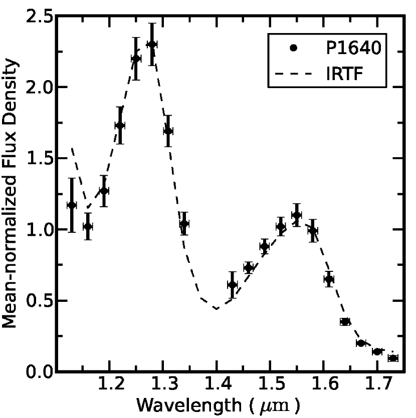
Figure 15: Disk-averaged spectrum of Titan extracted from a P1640 data cube, calibrated using the spectral response function in Figure 13. For comparison, a near-infrared spectrum of Titan acquired with IRTF/SpeX by Schaller is plotted alongside the P1640 data, after being binned and smoothed to the P1640 cube resolution. The IRTF/SpeX and P1640 Titan data were acquired two days apart, on 2009 March 13 and 15, respectively. Each spectrum is normalized to the mean of the points included in the plot. Channels 1, 10, 11, and 23 ($\lambda=1.10\>\mu\mbox{m},1.37\>\mu\mbox{m},1.40\>\mu\mbox{m, and }1.76\>\mu\mbox{m}$, respectively) were excluded due to varying telluric water absorption.

We expect the disk-averaged spectra acquired on these two dates to be similar. As Titan rotates over a 16-day period, in synchronicity with its orbit around Saturn, the near-infrared albedo observed from Earth (through the 1.3$~{}\mu$m and 1.6$~{}\mu$m methane “windows”) varies in a cycle with an amplitude on the order of 10%. This variation is caused by a change in surface features between the leading and trailing hemispheres (Lemmon et al., 1995). However, despite the 45 degree rotation of Titan with respect to Earth between the IRTF and P1640 observations, previous monitoring by several investigators indicates no significant albedo change between our specific pair of planetographic longitudes ($197\arcdeg$ and $243\arcdeg$) (Griffith et al., 1998). Furthermore, long-term monitoring of Titan’s albedo only occasionally reveals deviations from predicted reflectivity due to transient cloud features (e.g. Griffith et al., 1998; Schaller et al., 2009). The anticipated resemblance of the two spectra is confirmed in Figure 15: the average absolute difference between the IRTF and P1640 Titan data over the 19 channels used in Figure 15 is 7% of the mean flux, and most flux points agree within the error bars of the P1640 data. The only channel flux showing significant disparity with the IRTF data, centered at 1.13 $\mu$m, is located near the edge of a telluric water absorption trough, and therefore is more susceptible to calibration errors than most channels on the plot. For examples of M dwarf stellar spectra that have been measured from P1640 data cubes, see Zimmerman et al. (2010) and Hinkley et al. (2010).

6 Discussion

Starting from the economic constraint of limited detector area, the design of any integral field spectrograph must reach compromises between the competing parameters of spatial resolution, field of view, spectral resolution, and spectral range. For Project 1640, the need to Nyquist-sample the starlight speckle pattern inside the angular extent of the adaptive optics system “control radius” largely determined the balance of these tradeoffs. The other major factor was the overarching science goal of distinguishing astrophysically interesting features in the spectral energy distributions of young giant exoplanet atmospheres. Based on these considerations, the P1640 collaboration concluded on an IFU design that strongly favored a high density of spatial elements over spectral resolution, to a greater extreme than previous microlens-based integral field spectrographs. For example, the broadband mode of the TIGER IFU had 572 spatial elements dispersed at spectral resolution $R\>\sim\>370$, and the broadband mode of the OSIRIS IFU has 1024 spatial elements dispersed at $R\>\sim\>3400$ (Bacon et al., 1995; Larkin et al., 2006). P1640, by comparison, has 38,000 spatial elements with $R\>\sim\>40$, corresponding to over a factor of 30 increase in spatial elements, and a similarly substantial reduction in spectral resolution. Only two other IFUs will join P1640 in this operating regime in the next year: GPI and VLT-SPHERE—both designed for exoplanet imaging.

Since the properties of P1640 data are unusual even in the context of preceding IFUs, the instrument commissioning has required development of novel extraction and calibration approaches. Consider that each detector pixel width spans approximately 27.5 nm in spectral dispersion—4% of the instrument passband—and that the physical length of an individual microlens spectrum’s footprint is merely 0.5 mm at the focal plane. As such, great care has been required to accurately map the spectrograph focal plane data, in a manner that is resilient to subtle long-term changes in optical alignment. We described an answer to this problem in § 3, using a hierarchical fitting procedure to build a comprehensive, epoch-specific model of the full spectrograph focal plane. The last obstacle to securing the layout of the data, instrument flexure, must be dealt with individually for each exposure. Therefore, unlike the case of building the spectrograph focal plane model, we register each science spectrograph image “on the fly” inside the data pipeline, as explained in § 4.1.5.

The relatively long execution time required to build the spectrograph focal plane solution ($\sim$ 12 hours on a single high-performance workstation) means that it is sometimes necessary to rely on an outdated solution to extract data. Such will be the case, for example, during the first night of an observing run when the calibration Moon/sky image has not yet been acquired and fit. We know from the geometric evolution illustrated in Figure 7 that consequent errors in the positions of the spectra, along with other properties, will inevitably degrade the quality of the cube. However, for a preliminary inspection of data, and to check on instrument performance, the result will usually be acceptable. Recall that the spectrograph image registration uses a region of the image with the strongest signal to align the model. Therefore, under circumstances where the solution is old, the extraction will still tend to be fairly accurate near the brightest region of the image, but will progressively worsen towards the outskirts of the focal plane.

The main advantages of our weighted sum approach to IFU spectrum extraction, described in § 4.2.3, are simplicity and speed. Our reasoning behind using the spectrograph PSF itself to shape the weighting function is that it mimics the cross-dispersion profile of the spectrum. This way, along the middle horizontal row of the $3\times 3$ extraction box, we weight the detector samples by an estimate of their relative intensity (see Figure 11 for an example). Horne (1986) originally devised this strategy for extracting coarsely-sampled CCD spectra. He demonstrated that matching the weights to the expected cross-dispersion profile optimizes the fidelity of the extraction in the case where read noise is prevalent. This makes sense intuitively because we want detector samples with high count rates to have more influence than weak, noisy ones. Unlike the case of Horne’s spectrograph, however, we are dealing with many closely packed spectra, and so we are forced to truncate our weighting area to a region smaller than the actual extent of the PSF. We attempt to account for this in the weighting formula in Equation 21. Since this correction depends not just on the shape of the PSF but also the target spectrum, it is necessarily only an estimate, and can contribute errors on the order of a few percent to the spaxel value.

As compared to the cross-dispersion axis, for the dispersion axis there is more freedom in the choice of extraction weights. The tradeoffs here are signal-to-noise ratio per channel versus spectral resolution. Ultimately, for any weighted sum approach, the spectral resolution is limited by the width of the monochromatic IFU response along the dispersion axis. The spectrograph PSF fitting result plotted in the right-hand panel of Figure 3 shows this is about 2 detector pixels for P1640, which translates to $\sim$ 50 nm in the dispersion direction. For simplicity, we chose to remain with the PSF again to set the weights; the resulting cube spectra have a resolution of about 70 nm ($R\>\sim\>20$). In the future, it would be worthwhile to experiment with a hybrid weighting function that combines the cross-dispersion profile of the PSF with a different vertical profile, to investigate how much the spectral resolution can be improved. As one example of an alternative, Maire et al. (2010) propose extracting spectra from the GPI IFU by summing strictly along a single row/column of pixels in the cross-dispersion direction.

Another possible improvement to our data pipeline is a completely different extraction approach based on deconvolution or fitting. A well-designed fitting algorithm might disentangle the flux contributions of wavelengths with overlapping footprints. We have done a few experiments in this direction—for example, we applied the same MPFIT-based algorithm we used to model the microlens spectra in the Moon/sky calibration image (§ 3.2) to a science image. The results were of significantly poorer quality than our normal data cubes, partly as a consequence of not having the luxury to average the fit spectra over many microlenses, as we do with calibration images. In another program, two of our co-authors created a program that fits each spectrum cutout as a train of scaled PSFs, each one representing a different channel. While its implementation is not complete, this method shows promise of forming data cubes with slightly higher spectral resolution than the existing extraction. Since any fitting approach is inherently much slower than a weighted sum translation, one can imagine two cube extraction algorithms co-existing for different purposes: one as an offline procedure reserved for images of the greatest interest, and the other program applied to all P1640 data.

7 Conclusions

We have developed a collection of algorithms to reduce the data acquired by P1640, a coronagraphic integral field spectrograph designed for high contrast imaging. Our aim has been to describe our data pipeline software in enough detail that upcoming microlens-based imaging spectrograph projects can take advantage of our experience in treating closely packed, coarsely sampled spectra.

An essential element of our approach is an empirical model of the spectrograph focal plane image, based on calibration exposures in which the entire microlens array is illuminated, in turn, by broadband and monochromatic light. To derive a solution specific to each observation epoch, we fit a set of parameters describing each microlens spectrum (position, tilt, height, and overall signal amplitude). We use the resulting table of solved parameters to determine the extraction location on the focal plane for any given combination of microlens and wavelength, and hence build the data cube.

We implement the cube extraction with a weighted sum that optimizes the signal-to-noise ratio by mimicking the expected cross-dispersion profile, as constrained by the sub-pixel spectrograph image registration. Sources of error in the final data cube are cross-talk between adjacent microlens spectra, uncertainty in the spectrograph focal plane model, uncertainty in sub-pixel registration, and uncertainty in the determination of extraction weights. Nevertheless, based on an observation of Saturn’s moon Titan, we have demonstrated our ability to retrieve strong-featured near-infrared spectra to $\sim$ 5% accuracy. As our methods for handling this new form of data evolve, we expect P1640 to continue its pioneering role in high contrast astronomy.

References

- Bacon et al. (1988) Bacon, R., et al. 1988, European Southern Observatory Conference and Workshop Proceedings, 30, 1185
- Bacon et al. (1995) Bacon, R., et al. 1995, A&AS, 113, 347
- Beichman et al. (2010) Beichman, C. A., et al. 2010, PASP, 122, 162
- Beuzit et al. (2008) Beuzit, J.-L., et al. 2008, Proc. SPIE, 7014
- Bouchez et al. (2009) Bouchez, A. H., et al. 2009, Proc. SPIE, 7439
- Bracewell (2006) Bracewell, R. 2006, Fourier Analysis and Imaging (Springer)
- Brown (2007) Brown, M. G. 2007, Ph.D. Thesis
- Chauvin et al. (2010) Chauvin, G., et al. 2010, A&A, 509, A52
- Crepp et al. (2011) Crepp, J. R., et al. 2011, ApJ, 729, 132
- Dekany et al. (1997) Dekany, R. G., Wallace, J. K., Brack, G., Oppenheimer, B. R., & Palmer, D. 1997, Proc. SPIE, 3126, 269
- Fink & Larson (1979) Fink, U., & Larson, H. P. 1979, ApJ, 233, 1021
- Fixsen et al. (2000) Fixsen, D. J., Offenberg, J. D., Hanisch, R. J., Mather, J. C., Nieto-Santisteban, M. A., Sengupta, R., & Stockman, H. S. 2000, PASP, 112, 1350
- Griffith et al. (1991) Griffith, C. A., Owen, T., & Wagener, R. 1991, Icarus, 93, 362
- Griffith et al. (1998) Griffith, C. A., Owen, T., Miller, G. A., & Geballe, T. 1998, Nature, 395, 575
- Hinkley et al. (2007) Hinkley, S., et al. 2007, ApJ, 654, 633
- Hinkley et al. (2011) Hinkley, S., et al. 2011, PASP, 123, 74
- Hinkley et al. (2010) Hinkley, S., et al. 2010, ApJ, 712, 421
- Horne (1986) Horne, K. 1986, PASP, 98, 609
- Ives (2008) Ives, D., 2008, UK Astronomical Technology Centre Technical Memo: Threhold Limited NDR Algorithm
- Janson et al. (2008) Janson, M., Brandner, W., & Henning, T. 2008, A&A, 478, 597
- Larkin et al. (2006) Larkin, J., et al. 2006, Proc. SPIE, 6269
- Leconte et al. (2010) Leconte, J., et al. 2010, ApJ, 716, 1551
- Lemmon et al. (1995) Lemmon, M. T., Karkoschka, E., & Tomasko, M. 1995, Icarus, 113, 27
- Macintosh et al. (2006) Macintosh, B., et al. 2006, Proc. SPIE, 6272
- Manduca & Bell (1979) Manduca, A., & Bell, R. A. 1979, PASP, 91, 848
- Maire et al. (2010) Maire, J., et al. 2010, Proc. SPIE, 7735
- Markwardt (2009) Markwardt, C. B. 2009, Astronomical Society of the Pacific Conference Series, 411, 251
- McElwain et al. (2007) McElwain, M. W., et al. 2007, ApJ, 656, 505
- McElwain et al. (2008) McElwain, M. W., et al. 2008, SPIE Astronomical Instrumentation conference poster: An IFS for the Subaru Observatory HiCIAO system
- Miskey & Bruhweiler (2003) Miskey, C. L., & Bruhweiler, F. C. 2003, AJ, 125, 3071
- Mouillet et al. (2009) Mouillet, D., et al. 2009, Science with the VLT in the ELT Era, 337
- Offenberg et al. (2001) Offenberg, J. D., et al. 2001, PASP, 113, 240
- Oppenheimer & Hinkley (2009) Oppenheimer, B. R., & Hinkley, S. 2009, ARA&A, 47, 253
- Perrin et al. (2003) Perrin, M. D., Sivaramakrishnan, A., Makidon, R. B., Oppenheimer, B. R., & Graham, J. R. 2003, ApJ, 596, 702
- Pueyo et al. (2011) Pueyo, L., et al. 2011, ApJ, in prep.
- Racine et al. (1999) Racine, R., Walker, G. A. H., Nadeau, D., Doyon, R., & Marois, C. 1999, PASP, 111, 587
- Rayner et al. (2009) Rayner, J. T., Cushing, M. C., & Vacca, W. D. 2009, ApJS, 185, 289
- Rayner et al. (2003) Rayner, J. T., Toomey, D. W., Onaka, P. M., Denault, A. J., Stahlberger, W. E., Vacca, W. D., Cushing, M. C., & Wang, S. 2003, PASP, 115, 362
- Schaller et al. (2009) Schaller, E. L., Roe, H. G., Schneider, T., & Brown, M. E. 2009, Nature, 460, 873
- Sivaramakrishnan et al. (2001) Sivaramakrishnan, A., Koresko, C. D., Makidon, R. B., Berkefeld, T., & Kuchner, M. J. 2001, ApJ, 552, 397
- Soummer (2005) Soummer, R. 2005, ApJ, 618, L161
- Sparks & Ford (2002) Sparks, W. B., & Ford, H. C. 2002, ApJ, 578, 543
- Thatte et al. (2007) Thatte, N., Abuter, R., Tecza, M., Nielsen, E. L., Clarke, F. J., & Close, L. M. 2007, MNRAS, 378, 1229
- Zimmerman et al. (2010) Zimmerman, N., et al. 2010, ApJ, 709, 733