Flow-dependent unfolding and refolding of an RNA by nonequilibrium umbrella sampling

Abstract

Nonequilibrium experiments of single biomolecules such as force-induced unfolding reveal details about a few degrees of freedom of a complex system. Molecular dynamics simulations can provide complementary information, but exploration of the space of possible configurations is often hindered by large barriers in phase space that separate metastable regions. To solve this problem, enhanced sampling methods have been developed that divide a phase space into regions and integrate trajectory segments in each region. These methods boost the probability of passage over barriers, and facilitate parallelization since integration of the trajectory segments does not require communication, aside from their initialization and termination. Here we present a parallel version of an enhanced sampling method suitable for systems driven far from equilibrium: nonequilibrium umbrella sampling (NEUS). We apply this method to a coarse-grained model of a 262-nucleotide RNA molecule that unfolds and refolds in an explicit flow field modeled with stochastic rotation dynamics. Using NEUS we are able to observe extremely rare unfolding events that have mean first passage times as long as 1.4 s ($3.4\times 10^{13}$ dynamics steps). We examine the unfolding process for a range of flow rates of the medium, and we describe two competing pathways in which different intramolecular contacts are broken.

I Introduction

Nonequilibrium measurements on biological macromolecules, such as mechanical force-induced unfolding Liphardt et al. (2001) and flow-based analogs Lin et al. (2009), have emerged as a powerful complement to equilibrium studies. Indeed, it now possible to follow the evolution of distances through fluorescence resonance energy transfer (FRET) simultaneously with forces through optical traps Comstock et al. (2011). While these measurements provide unprecedented experimental data on the stochastic dynamics of individual molecules, they still only probe at most a few degrees of freedom among many. Molecular dynamics simulations, which provide complete information about the positions of all participating particles subject to the assumptions of the model, have proven to be a valuable tool for interpreting these data Sotomayor and Schulten (2007). However, the time scales for conformational change are often long compared with elementary fluctuations, which makes waiting for the events of interest to occur spontaneously under conditions representative of experimental ones prohibitively computationally costly. To accelerate convergence, many simulation studies employ unrealistically extreme nonequilibrium conditions (see discussion in Hu et al. Hu et al. (2006)).

Alternatively, enhanced sampling methods can be used to improve exploration of phase space and focus computational effort on low probability regions of mechanistic importance, such as transition states. The most widespread such methods Frenkel and Smit (2002); Dellago and Bolhuis (2009); E and Vanden-Eijnden (2010) rely on the fact that the statistics of equilibrium systems are known a priori, which prevents the applicability of such methods to nonequilibrium situations. However, there now exist methods that can enhance the sampling of low probability regions without relying on equilibrium properties of the system Allen et al. (2005, 2006a, 2006b, 2009); Warmflash et al. (2007); Dickson et al. (2009a, b); Dickson and Dinner (2010); Huber and Kim (1996); Zhang et al. (2007); Bhatt et al. (2010); Bhatt and Zuckerman (2010). Although these methods differ in detail, the essential idea in all of them is to harvest segments of unbiased dynamics trajectories such as to achieve relatively uniform sampling of different regions of a space of physically relevant degrees of freedom (order parameters). The acceleration of convergence follows from the fact that each trajectory segment need only traverse a small portion of the space of order parameters, across which the probability is relatively uniform.

We have been developing one such method: nonequilibrium umbrella sampling (NEUS) Warmflash et al. (2007); Dickson et al. (2009a, b); Dickson and Dinner (2010). In this paper, we present a streamlined version of the algorithm with improved convergence properties. The most significant change is the explicit association of a weight with each saved copy of the system, motivated by the weighted ensemble method Huber and Kim (1996); Zhang et al. (2007, 2010); Bhatt et al. (2010); Bhatt and Zuckerman (2010). The fact that many trajectory segments are integrated independently makes the method highly parallelizable, and we detail and implement a strategy that can provide excellent scaling to large numbers of processors.

We use the method to simulate partial unfolding and refolding of a coarse-grained model of a 262-nucleotide RNA molecule in the presence of a flow field. Our interest in this system comes from single-molecule studies of FRET between probes on the L18 loop and 3^′ terminus of the catalytic domain of the RNase P RNA from Bacillus stearothermophilus Smith et al. (2008); Qu et al. (2008); Li et al. (2009). In these studies, the molecule was tethered in a microfluidic channel to enable relatively rapid changes in magnesium ion concentration, and this led to the question of whether flow contributed to the dynamics observed Li et al. (2009). Here, we show that there are two competing unfolding pathways, the likelihoods of which depend on the rate of flow of the solution. We compare these results with reversible unfolding simulations (without a net flow).

II Methods

II.1 Algorithm

As we show, the events of interest are on the time scale of milliseconds to seconds, while straightforward simulations of the coarse-grained model are limited to tens of microseconds. Thus enhanced sampling is needed. Here, we describe the version of nonequilibrium umbrella sampling (NEUS) Warmflash et al. (2007); Dickson et al. (2009a, b); Dickson and Dinner (2010) used in the present study. To this end, we summarize the overall strategy, and then we describe the phases of the simulation and parallelization; differences from earlier versions of the algorithm and competing methods are noted.

II.1.1 Overall strategy

The sampling is guided by a set of physically relevant variables (“order parameters”). Ideally, these order parameters will describe the slow dynamics in the system, and the remaining degrees of freedom will relax relatively fast. In this work, we employ a single order-parameter that quantifies the total number of intramolecular contacts (Section II.2). However, we explicitly separate the “forward” (unfolding) and “backward” (refolding) transition path ensembles as in Dickson et al. Dickson et al. (2009b). This allows the sampling of the orthogonal degrees of freedom to differ between the two ensembles (i.e., allows for separate unfolding and refolding pathways), and it enables the calculation of transition rates between basins.

For the simulations, we divide the space of order parameters into regions, which need not be uniform in size. Each region contains one or more copies of the system (walkers) that evolve independently according to the natural dynamics of the system, and we associate with that copy a weight for contributing to averages. When a copy of the system attempts to leave its region, the configuration is saved to a list of entry points for the neighboring region, along with the weight of the copy. When a neighboring list is full, the oldest saved configuration is overwritten and its weight is distributed over the remaining points in the list in a manner that does not affect their relative probabilities of being chosen. The copy is then restarted from a saved configuration, $i$, which is chosen from one of its region’s lists with likelihood proportional to its weight ($w_{i}$). The weight of this point is then partitioned between the active and saved copies: $\gamma w_{i}$ ($\gamma\in(0,1]$) is given to the active copy, and the rest, $(1-\gamma)w_{i}$, remains associated with the saved entry point. Note that $\gamma=1$ results in straightforward dynamics, or a single, continuous trajectory. Here we use $\gamma=0.9$. The incorporation of this feature in the NEUS algorithm is motivated by the (equal) partitioning of the probability when a trajectory branches in the weighted ensemble (WE) method Huber and Kim (1996); it ensures conservation of the starting probability and suppresses artificial amplification of particular trajectories. As a result, we are able to obtain converged results with only one set (lattice) of regions in the extended space as opposed to two as in previous work Warmflash et al. (2007); Dickson et al. (2009a, b).

II.1.2 Initialization

A common situation is that one is interested in studying a transition between two or more states but one knows the configuration of the system in only one of the stable states. This situation applies here to the RNA-under-flow system, since we know the folded configuration but not the most likely unfolded configurations. Although in principle one could start the simulation in each region using any configuration consistent with the allowed order parameter values, in practice it is best to start with a distribution of structures that is as consistent as possible with the physically weighted dynamics to avoid introducing unnecessary errors that take time to be corrected. To this end, we progressively activate the regions in a manner similar to Forward Flux Sampling (FFS) Allen et al. (2009) as follows.

We start by running an unconstrained simulation that is initialized in the known stable configuration. During this simulation, we record the configuration each time the system crosses a boundary of a region but do not reset the configuration. These configurations serve as the initial entry (i.e., resetting) points for the regions visited, and all such configurations are assigned equal weight. Following the unconstrained simulation, we begin the umbrella sampling simulation starting from saved entry points in each region that has at least one such point, employing and updating the copy weights as described above. Regions that were not visited previously are activated once entry points for them are obtained. As the simulations proceed, regions of lower and lower probability are activated by their neighbors, and trajectories emerge from the original stable state. Once all the regions are activated, we are able to concurrently sample the entire order parameter space of interest, using only points that resulted directly from the starting distribution.

In the present study, the progressive initialization of regions accounts for about 2% of the total simulation time. The sampling procedure employed here further differs from FFS in that it does not explicitly require a notion of forward progress and thus can be used with sampling regions that are defined by an arbitrary number of order parameters. By the same token, trajectories are terminated when they cross any boundary, not only a forward one. This distinction is of practical importance when the dynamics do not lead rapidly back to the starting basin (see Dickson et al. Dickson and Dinner (2010) for further discussion).

II.1.3 Weight redistribution

The algorithm as described is in principle complete. Indeed, it is very similar to the WE method except that (i) it permits strict control of the number of copies in a region (including only limiting it to one) and (ii) differs in the details of weight partitioning when resetting (branching) and redistributing when overwriting (pruning). However, the transfer of weight between regions of high probability can be very slow when the weight must pass through a bottleneck region of low probability. This is because a very large number of low probability walkers are required to add up to a significant change of weight in a high probability region. This convergence issue arises despite the fact that the time for initial exploration of the space decreases with increases in the number of regions, as in any umbrella sampling procedure Chandler (1987); Frenkel and Smit (2002).

To accelerate convergence after the initialization phase, we periodically use the interface-to-interface crossing statistics to predict statistical weights for each region ($\{W_{i}\}$), and scale the weights of the entry points in each region, $i$, such that their sum is equal to $W_{i}$. Here, the weights are obtained from a modified version of the scheme in Vanden-Eijnden and Venturoli Vanden-Eijnden and Venturoli (2009), where the total flux into a region is set equal to the total flux out of a region. To this end, we accumulate a transition matrix, $\mathbb{T}$: each off-diagonal element $t_{ij}$ is the number of transitions observed from region $j$ to region $i$ in the last weight update period, and each diagonal element $t_{ii}=-\sum_{j}t_{ji}$. We then solve the equation $\mathbb{T}{\bf W}={\bf 0}$ for the weight vector ${\bf W}$ by using singular value decomposition to compute the nullspace of $\mathbb{T}$, which is the single nontrivial solution ${\bf W}$. Here, we perform this operation periodically throughout the simulation, as in previous NEUS studies Dickson et al. (2009b); Vanden-Eijnden and Venturoli (2009); this contrasts with the study by Bhatt et al. Bhatt et al. (2010) in which a single such step is used to pre-condition the simulation and then flux balance is used to check convergence.

II.1.4 Parallelization

The simulations of the copies of the system require only limited communication. As such, NEUS and methods like it lend themselves well to parallelization. However, we find that they benefit from careful implementation on high performance computers. All simulations for the present study are run on parallel architectures using the Global Arrays toolkit Nieplocha et al. (1996), which implements a global address space programming model in which processes can access remote data using one-sided communication. One-sided communication is particularly useful in this case, since the timing of boundary crossing events is not predictable. The global address space also enables one to distribute the storage of a large set of region entry points across the memory of many compute nodes. The entry points for each region, the region weights, boundary crossing statistics and sampling histogram data are all stored as global arrays. These arrays can be modified by any process using “put” functions and “get” functions, where locks are used to enable atomic updates of global data (modifications of the entry point lists, for instance) that prevent processes from concurrently accessing the same region of a global array.

Although the dynamics of the copies are simulated essentially without communication once they are initialized, NEUS still periodically requires some collective operations, such as weight updates, and the computation of rates and probability distributions. To allow for such operations, we break down the simulation into “cycles” of computation, at the end of which all processes are synchronized. Within the cycles, the work is distributed among the processes as follows. When a process is finished running a trajectory segment, it queries how many steps have been run in each region $k$ so far this cycle ($N_{k}$), and it uses the results to decide in which region to run the next trajectory segment. Specifically, it chooses to start a trajectory in region $j$ with probability

$$P_{j}=\frac{N_{\text{steps}}-N_{j}}{\sum_{k}(N_{\text{steps}}-N_{k})},$$ (1)

where $N_{\text{steps}}$ is the number of steps to be run in each region per cycle. A trajectory is run until either the counter in its region reaches $N_{\text{steps}}$ (upon which the current configuration of the system is saved to the entry point list as a simple means of maintaining it), and a computational cycle ends when all counters reach $N_{\text{steps}}$.

II.2 Model

The system is a model of the catalytic domain of RNase P RNA from Bacillus stearothermophilus. To make the simulations tractable, we use a coarse-grained representation that averages over the atomic structure and dynamics, while taking into account the secondary and tertiary interactions that stablize the native state: the self-organized polymer (SOP) model Hyeon and Thirumalai (2007). In the SOP model, each nucleotide of the RNA is treated as a bead, and the beads interact through potentials that depend on the known native structure. The potential defining the model is the sum of a finitely extensible nonlinear elastic (FENE) potential that connects adjacent beads Kremer and Grest (1990) ($V_{\text{FENE}}$); a Lennard-Jones attraction between beads that has a minimum at the native structure distance ($V^{\text{att}}_{\text{nb}}$); pairwise non-bonded repulsions scaling as $r^{-6}$, which locally straighten the chain and mimic steric repulsions between nucleotides ($V^{\text{rep}}_{\text{nb}}$); and a Weeks-Chandler-Andersen Weeks et al. (1971) (WCA) repulsion between each bead and the wall at $y=0$ ($V^{\text{wall}}$). The total potential function is

$$V_{\text{T}}=V_{\text{FENE}}+V^{\text{att}}_{\text{nb}}+V^{\text{rep}}_{\text{nb}}+V_{\text{wall}}\\$$

with

$$V_{\text{FENE}} =-\sum_{i=1}^{N-1}\frac{k}{2}R_{0}^{2}\log\left(1-\frac{(r_{i,i+1}-r^{0}_{i,i+1})^{2}}{R_{0}^{2}}\right)$$

$$V^{\text{att}}_{\text{nb}} =\sum_{i=1}^{N-3}\sum_{j=i+3}^{N}\epsilon_{h}\left[\left(\frac{r_{ij}^{0}}{r_{ij}}\right)^{12}-2\left(\frac{r_{ij}^{0}}{r_{ij}}\right)^{6}\right]\Delta_{ij}$$

$$V^{\text{rep}}_{\text{nb}} =\sum_{i=1}^{N-2}\epsilon_{l}\left(\frac{\sigma^{*}}{r_{i,i+2}}\right)^{6}+\sum_{i=1}^{N-3}\sum_{j=i+3}^{N}\epsilon_{l}\left(\frac{\sigma}{r_{ij}}\right)^{6}(1-\Delta_{ij})$$

$$V_{\text{wall}} =\sum_{i=1}^{N}H(2^{1/6}\sigma_{\text{WCA}}-y_{i})\times 4\epsilon_{l}\left[\left(\frac{\sigma_{\text{WCA}}}{y_{i}}\right)^{12}-\left(\frac{\sigma_{\text{WCA}}}{y_{i}}\right)^{6}\right],$$ (2)

where $r_{ij}$ is the distance between residues $i$ and $j$, and $r^{0}_{ij}$ is their distance in the native structure. We set the parameters in (II.2) to those in Hyeon and Thirumalai Hyeon and Thirumalai (2007), namely $R_{0}=0.2$ nm, $\epsilon_{h}=0.7$ kcal/mol, and $\epsilon_{l}=1.0$ kcal/mol; we set $\sigma=7$ Å to ensure noncrossing of the chain, and we set $\sigma^{*}=3.5$ Å to prevent the flattening of helical structures. In $V_{\text{wall}}$, $\sigma_{\text{WCA}}=2$ Å, and $H(x)$ is a Heaviside function equal to $0$ for $x<0$ and $1$ for $x>0$. The equation of motion for the polymer is integrated with the Velocity-Verlet algorithm with time step $\delta t=40$ fs.

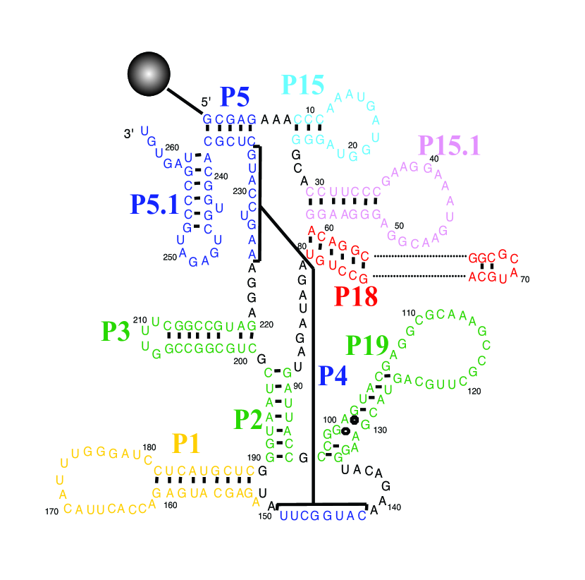
The native, folded structure was constructed from the crystal structure for the full RNase P RNA Kazantsev et al. (2005). The coordinates of the catalytic domain (262 residues) were isolated from the full structure (417 residues), and coarse-graining into beads was carried out by replacing the coordinates of each residue with its center of mass. Unstructured residues, which did not have crystal structure coordinates (in Figure 1, residues 161-181 in P1, 15-20 in P15, 64-73 in P18, and 106-125 in P19) were added by introducing the appropriate number of beads into the sequence, separated by the average bead-bead distance (about 5 Å); these unstructured residues have no contacts. The structure was allowed to relax to its minimum energy by integrating without a random force so that the added unstructured residues form simple loops. Using this structure, we consider a native contact to exist ($\Delta_{ij}=1$) between all pairs of residues $i$ and $j$ with $|i-j|>2$ and distance less than $R_{C}=1.4$ nm in the native structure; for all other pairs $\Delta_{ij}=0$.

The solvent in the simulation is modeled using the stochastic rotation dynamics method Malevanets and Kapral (1999); Ihle and Kroll (2001); Lamura et al. (2001); Allahyarov and Gompper (2002), in which the solvent is represented by a large number of infinitesimal particles that are grouped into cubic “interaction cells”. Each step of the algorithm comprises two parts: (1) free streaming, in which the position of particle $i$ (${\bf r}_{i}$) is updated according to ${\bf r}_{i}(t+\Delta t)={\bf r}_{i}(t)+{\bf v}_{i}(t)\Delta t$ where ${\bf v}_{i}$ is the velocity at time $t$ and $\Delta t=150\delta t$ is the solvent time step and (2) “collision”, in which ${\bf v}_{i}(t+\Delta t)={\bf v}_{\rm cell}(t)+\Omega[{\bf v}_{i}(t)-{\bf v}_{\rm cell}]$ where ${\bf v}_{\rm cell}$ is the average velocity of particles in the cell containing $i$, and $\Omega$ is a stochastic rotation matrix which rotates vectors around a random axis by $\pm\alpha$, a fixed angle, with equal likelihood. Here we use $\alpha=0.243\pi$, which in combination with the other parameters used here for the solvent, gives a viscosity of $0.8$ g/m/s, which is approximately the viscosity of liquid water at our simulation temperature (300 K). The viscosity was calculated using Equations 10 and 14 of Kikuchi et al.Kikuchi et al. (2003).

Figure 1: Secondary structure of the RNA molecule. In the simulation, the 5^′ end of the molecule is attached to a tether (black sphere), that prevents the molecule from moving along with the flow. The index of every tenth residue is shown.

We allow the solvent to influence the RNA by including the polymer beads in the collisions, as in Webster and YeomansWebster and Yeomans (2005). This is done using

$${\bf v}_{\rm cell}(t)=\frac{\sum_{\rm cell}m{\bf v}_{i}(t)+\sum_{\rm cell}M{\bf V}_{i}(t)}{N_{\rm cell}^{\rm solv}m+N_{\rm cell}^{\rm poly}M}$$ (3)

where $m=32$ amu is the mass of the solvent particles (chosen to make a solvent mass density of 1 g/mL), and $M=300$ amu is the mass of the residues, compared with a range in mass for RNA nucleotides of 320 to 360 amu. ${\bf V}_{i}(t)$ is the velocity vector for residue $i$, and the sum is over all particles in the cell.

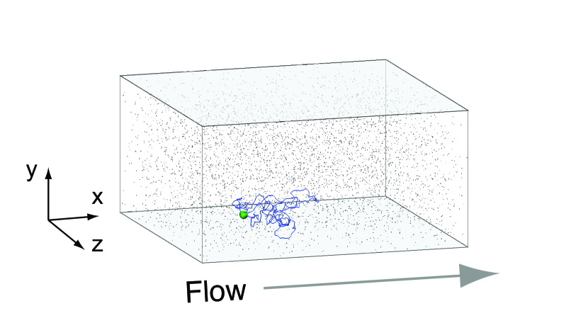
We use periodic boundary conditions in the $x$ and $z$ directions, reflective walls at $y=0$ and $y=L_{y}$, and drive the solvent to flow in the positive $x$ direction (Figure 2). The dimensions of the box are $L_{x}=L_{z}=384$ Å and $L_{y}=192$ Å. The interaction cells are cubic with side length 8 Å, which was chosen to be comparable with the average distance traveled by a solvent particle in a time $\Delta t$. Following previous work, we shift the lattice periodically to avoid artifacts Ihle and Kroll (2001) and employ the generalized bounce back rule for partially filled cells along the $y=0$ and $y=L_{y}$ edges Lamura et al. (2001). An extra FENE interaction is added between the 5^′ terminus and the tether point, located at (120 Å, 25 Å, 192 Å) to prevent the molecule from moving along with the flow.

Figure 2: The simulation cell. The boundaries at $y=0$ and $y=L_{y}$ have reflective boundary conditions, while the others are periodic. The tether point is shown as a large green sphere, and the RNA molecule is in blue. $5000$ of the $503200$ solvent molecules are shown here. A flow is induced in the positive $x$-direction by applying a constant acceleration to the solvent particles, which in turn causes extension of the RNA molecule in that direction.

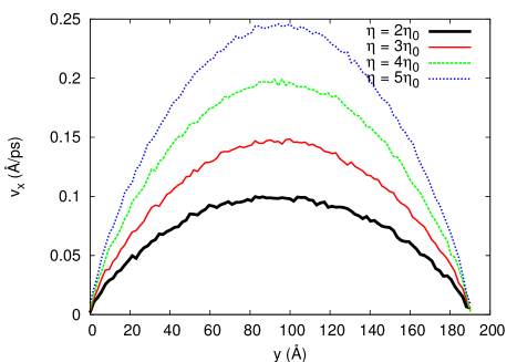
The flow is introduced by accelerating each solvent particle that is not in the $y=0$ or $y=L_{y}$ boxes in the $x$ direction after every rotation step according to $v_{x}^{i}\rightarrow v_{x}^{i}+\eta\Delta t$, where $\eta$ is an acceleration parameter. The $\eta$ values used here range from $2\eta_{0}$ to $5\eta_{0}$, where $\eta_{0}=625$ Å/fs². Figure 3 shows average flow profiles, obtained without the polymer. The Péclet number is the ratio of advective motion to thermal diffusive motion, given by

$$\text{Pe}=\frac{L\bar{v}_{x}}{D}$$ (4)

where $L=8$ Å is the characteristic length, $\bar{v}_{x}$ is the average velocity of the solvent in the $x$ direction, and $D$ is the self-diffusion constant of a single residue calculated in zero flow. Here, Pe ranges from $1.4\times 10^{-2}$ to $3.9\times 10^{-2}$, indicating that at all values of $\eta$ we examine, thermal motion is much stronger than advective motion (i.e., $\text{Pe}\ll 1$). Prior to the start of the umbrella sampling simulation, the solvent was equilibrated without the polymer until the flow profiles converged; this required $40$ ns, which corresponds to roughly $6700$ streaming steps.

Figure 3: Flow velocity profiles. For each flow rate examined here, we plot the average velocity of solvent molecules in the $x$-direction as a function of $y$. These were obtained without the polymer. The profiles are parabolic, due to the presence of reflective walls at $y=0$ and $y=L_{y}$.

II.3 Order parameter

The order parameter that we use here to distinguish between the folded and unfolded states is an estimate of the number of native contacts that are made in a given configuration:

$$N_{c}(t)=\sum_{i,j}\Delta_{ij}\phi(r_{ij}(t))$$ (5)

where $r_{ij}(t)$ is the distance between the two residues at time $t$, $\phi(r_{ij})$ is a function that is equal to $1$ when the contact is satisfied ($r_{ij}<a_{f}r^{0}_{ij}$), $0$ when the contact is not satisfied ($r_{ij}>2a_{f}r^{0}_{ij}$), and varies between $0$ and $1$ for intermediate values as $(a_{f}r^{0}_{ij}/r_{ij})^{8}$, where the exponent was chosen to make the jump at $r_{ij}=2a_{f}r^{0}_{ij}$ small, while being efficient to compute. The constant $a_{f}=2.0$ was used here; we found that it provided a good balance between limiting sensitivity to fluctuations within stable states (large $a_{f}$) and detecting early unfolding activity (small $a_{f}$). A plot of $\phi(r_{ij})$ is shown in Figure 4.

Figure 4: The function $\phi(r_{ij})$ that is used to calculate the order parameter $N_{c}$.

We use this order parameter to define “folded” and “unfolded” basins as $N_{c}\geq N_{\text{fold}}$ and $N_{c}\leq N_{\text{unfold}}$ respectively. We separate the transition path ensemble into two subensembles: the unfolding ensemble and the refolding ensemble. By tracing the dynamics of each copy back through the saved entry points, we can classify each copy as being on a trajectory that originates in either the folded or unfolded basin. The unfolding ensemble is composed of all trajectories that originate in the folded basin (regardless of whether they reach the unfolded basin or return to the folded one), and the refolding ensemble is composed of all trajectories that originate in the unfolded basin (regardless of whether they reach the folded basin or return to the unfolded one). In other words, the ensembles are defined by the histories rather than futures of walkers. Each ensemble has its own set of regions that span the order parameter space. As shown in Dickson et al. Dickson et al. (2009b), the two sets of regions can be seen as a single set of nonoverlapping regions in an extended space, and transition rates between the basins can be obtained by calculating fluxes in this extended space.

II.4 Simulation details

In the simulations presented here, the saved entry point lists for each region are divided into two lists of 250 points each. One list is dedicated to points coming from the right (higher $N_{c}$) and the other to points coming from the left (lower $N_{c}$). This helps ensure that the left and right ensembles are both well described. An element of a list consists of the positions and velocities of all the residues of the molecule, as well as forces from the previous step of the Velocity-Verlet algorithm. Along with these data we store the weight of the trajectory, and a time counter that is used to determine when to perform solvent streaming steps. We found it unnecessary to store the coordinates of the solvent along with the flux input point, since the solvent relaxes almost instantaneously to the presence of the polymer (data not shown), as there are no steric interactions between the polymer and solvent.

In the work below, a cycle constitutes 2000 RNA time steps in each active sampling region. We allow 3000 cycles for progressive initialization (Phase II), and another 3000 cycles with global weight updates (Phase III). We perform a global weight update at the beginning of Phase III, and again every 600 cycles after that. As will be discussed below, the number of sampling regions used depends on the pathway observed, and is either 40 or 84 in each direction, for a total of either 80 or 168 regions in the extended space. The total number of sampling steps depends on how fast regions are initialized in Phase II, but it is less than $9.6\times 10^{8}$ in the 40 region case and less than $2.02\times 10^{9}$ in the 84 region case.

III Results

The RNA-under-flow system was examined at four different flow accelerations: $\eta=2\eta_{0}$, $3\eta_{0}$, $4\eta_{0}$ and $5\eta_{0}$. These correspond to Péclet numbers of $1.5\times 10^{-2}$, $2.3\times 10^{-2}$, $3.0\times 10^{-2}$ and $3.9\times 10^{-2}$, respectively. These numbers indicate that thermal motion is much more important than advective motion (i.e., $\text{Pe}\ll 1$), but, as we show, there are significant flow effects. We also examine the equilibrium case: $\eta=0$. For each flow rate we obtained folding and unfolding rates, probability distributions for the numbers of native contacts, and a set of input structures to each umbrella sampling region, from which we can reconstruct folding and unfolding pathways. As detailed below, the folded and unfolded basins were defined by our measure of the number of native contacts, $N_{c}$ (Section II.3).

III.1 Competing unfolding pathways

Interestingly, we found two competing reaction pathways for the molecule. One pathway (“path M”) occurred by breaking contacts in the middle of the molecule, in and around the P1 loop (residues 150-190, see Figure 1), while the other (“path E”) occurred by breaking contacts in and around the P5 region (residues 1-5 and 234-238), which is near the tethered end. We obtained pathways in duplicate for each value of $\eta$, and found a dependence of the pathway on the flow pressure. For $\eta\leq 3\eta_{0}$ we observed path M in both trials, for $\eta=5\eta_{0}$ we observed path E in both trials, and for $\eta=4\eta_{0}$ we observed path M and path E each once, which suggests that path E is more probable for higher flow rates, and that $\eta=4\eta_{0}$ is close to a transition point where the relative probabilities of the two pathways cross over.

The folded basin for both pathways was located at $N_{c}\geq 960$, and the unfolded basin was placed at the first metastable unfolded structure we encountered along each unfolding pathway. Although these structures could be intermediates to further unfolded states, we will call these structures “unfolded”, and their corresponding basins “unfolded basins”. For path M, we set the unfolded basin to $N_{c}\leq 900$, and for path E we set the unfolded basin to $N_{c}\leq 834$. In both pathways, we define the regions in $N_{c}$ with an even spacing of $\Delta N_{c}=1.5$, giving us 40 regions for the unfolding pathway in path M, and 84 regions for the unfolding pathway in path E. There are an equal number of regions in the refolding pathways in both cases, giving us a total of 80 and 164 regions in paths M and E, respectively.

III.2 Pathway analysis

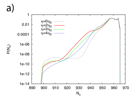
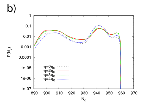
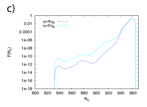
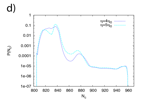
Probability distribution functions of the order parameter $N_{c}$ are shown in Figure 5, for both pathways, and for both the unfolding and refolding ensembles. For path M, we show histograms for $\eta=2\eta_{0}$, $3\eta_{0}$ and $4\eta_{0}$. In the unfolding ensemble (Figure 5a), there is a strong peak at $N_{c}=960$ for all flow rates, corresponding to the native state. In the refolding ensemble (Figure 5b), there is a peak at $N_{c}=907$ corresponding to the first metastable unfolded state, and an intermediate unfolded state at $N_{c}=942$. For path E, we show histograms for $\eta=4\eta_{0}$ and $5\eta_{0}$. Here, the refolding ensemble (Figure 5d) shows that there are two metastable states near the unfolded basin with peaks at $N_{c}=820$ and $N_{c}=838$, as well as an intermediate at $N_{c}=875$.

Figure 5: $N_{c}$-histograms for both pathways. (a)-(b) The unfolding and refolding ensembles of path M, respectively. Flow pressures $\eta/\eta_{0}=0$, $2$, $3$ and $4$ are shown to be very similar. (c)-(d) The unfolding and refolding ensembles of path E, respectively. Flow pressures $\eta/\eta_{0}=4$ and $5$ are shown. From (c) it is clear that this pathway is much more probable for $\eta/\eta_{0}=5$ than for $\eta/\eta_{0}=4$, and occurs approximately $100$ times faster.

Figure 6: The contact map that is representative of the folded state for all flow rates examined here. This map was obtained using structures from entry points for the region in the unfolding ensemble with the highest value of $N_{c}$, at the end of a $\eta=2\eta_{0}$ simulation.

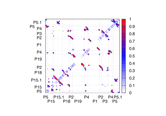
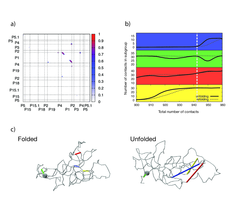
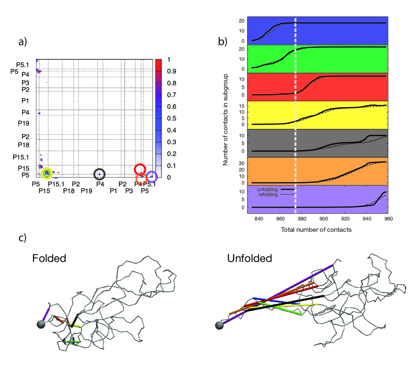
To characterize structures along the pathways, we construct contact difference maps by subtracting average contact maps for the unfolded states from that for the folded state shown in Figure 6. The contact maps for the unfolded states are computed using the structures from the saved entry point lists for the regions in the refolding ensembles with the lowest values of $N_{c}$, and similarly a contact map for the folded state is computed using structures from the saved entry point list for the region in the unfolding ensemble with the highest value of $N_{c}$. The contact difference maps are shown in Figures 7a and 8a along with characteristic structures of the folded and unfolded states (Figures 7c and 8c). Based on their kinetic behavior, we divide the contacts into groups and track the population of each group as a function of $N_{c}$ (Figures 7b and 8b).

The vertical lines in Figures 7b and 8b show the metastable states along the refolding pathway. For path M the local maximum at $N_{c}=942$ is associated with the reformation of contacts in the P1 loop (subgroup 3). For path E the local maximum at $N_{c}=875$ is associated with the reformation of contacts in the P15 loop (subgroups 2 and 4). For path M we observe that the unfolding and refolding ensembles do not overlap. Specifically, contacts between the endpoints of the molecule (P5-P5.1 contacts) break and reform along the unfolding pathway, but remain intact during the refolding pathway. In this regard, it is important to keep in mind that the unfolding ensemble, as defined in Section II.3 contains both folded-to-unfolded trajectories and folded-to-folded trajectories. The fact that the feature in question appears in analogous calculations for the reversible system ($\eta=0$), where there can be no hysteresis, suggests that the P5-P5.1 contacts are broken along folded-to-folded trajectories, and that this process is not a causal part of the path M unfolding mechanism.

Figure 7: Analysis of path M. (a) Contact difference map obtained by subtracting the contact map of the unfolded state from the contact map of the folded state. This reveals the contacts which are broken along the pathway. The colored circles show the division of these contacts into subgroups. (b) The number of contacts in each subgroup is plotted as a function of the total number of contacts averaged over the $\eta=2\eta_{0}$ ensemble of structures. These curves are computed using structures in the saved entry point lists for every region in both the unfolding and refolding ensembles, at many times throughout Phase III of the simulation. The vertical lines show the metastable states along the refolding pathway. (c) Representative contacts from each group are shown on the RNA molecule for the folded and unfolded states.

Figure 8: Figure 8. Analysis of path E. See descriptions of panels in Figure 7. (a) Contact difference map. The green and yellow circles define subgroups of secondary and tertiary contacts within the region, respectively. (b) Note in this pathway that there is no hysteresis between the unfolding and refolding pathways.

III.3 Transition rates

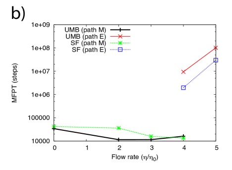
The mean first passage times of the unfolding processes are given in Tables 1 and 2 for paths M and E respectively. These range from $6.8$ to $460$ ms for path M and $590$ to $1400$ ms for path E. As each dynamics step is $40$ fs, these correspond to numbers of dynamics steps between $1.7\times 10^{11}$ and $3.4\times 10^{13}$. The unfolding and refolding MFPTs are shown as functions of flow pressure in Figure 9.

Table 1: Unfolding and refolding mean first passage times for path M, obtained for $\eta=0$, $2\eta_{0}$, $3\eta_{0}$ and $4\eta_{0}$. For refolding pathways, the MFPTs from umbrella sampling (NEUS) and straightforward sampling (SF) are shown.

$\eta/\eta_{0}$	Unfolding (NEUS) (in ms)	Refolding (NEUS) (in ns)	Refolding (SF) (in ns)
$0$	$220$	$1.5$	$1.7$
$2$	$6.8$	$0.82$	$1.4$
$3$	$110$	$0.85$	$0.6$
$4$	$460$	$0.91$	$0.5$

Table 2: Unfolding and refolding mean first passage times for path E, obtained for $\eta=4\eta_{0}$ and $5\eta_{0}$. For refolding pathways, the MFPTs from umbrella sampling (NEUS) and straightforward sampling (SF) are shown.

$\eta/\eta_{0}$	Unfolding (NEUS) (in ms)	Refolding (NEUS) (in $\mu$s)	Refolding (SF) (in $\mu$s)
$4$	$1400$	$0.38$	$0.08$
$5$	$590$	$4.1$	$1.2$

Figure 9: Figure 9. (a) Mean first passage times for unfolding events, as predicted by NEUS. For path M, this is the average number of steps required to go from $N_{c}=960$ to $N_{c}=900$, and for path E, this is the average number of steps to go from $N_{c}=960$ to $N_{c}=834$. (b) Mean first passage times for refolding events, comparing umbrella sampling (UMB) and straightforward trajectories (SF). These agree to within an order of magnitude.

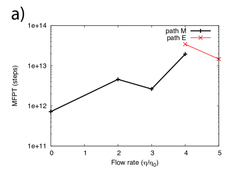
The unfolding rates show counter-intuitive behavior for path M. The MFPT increases with the flow rate; unfolding becomes more difficult as greater flow is applied to the system. Such behavior could be caused by larger flow gradients at the surface causing nucleotides in the P1 loop to be pushed together rather than pulled apart. For path E, the MFPT for unfolding decreases with increasing flow rate, although we only have two data points to establish this trend. We note that the MFPTs for path M and path E are not directly comparable, since the former measures the average amount of time to go from $960$ to $900$ contacts, and the latter measures the average amount of time to go from $960$ to $834$ contacts.

The rates of refolding are also given in Tables 1 and 2. They are much faster, which makes comparisons with straightforward trajectories possible. We use the umbrella sampling saved entry point lists to generate an initial unfolded ensemble for each flow rate, since umbrella sampling is our only access to physically weighted unfolded states. We compare refolding rates for both pathways and all flow pressures, which agree to within an order of magnitude. For path M, the refolding MFPT is short ($\sim 1$ ns), and relatively constant with varying flow rate. For path E, the refolding MFPTs are longer, since the unfolded state is more stable, and increase with increasing flow rate: $0.3$ $\mu$s for $\eta=4\eta_{0}$, and $4.1$ $\mu$s for $\eta=5\eta_{0}$. This behavior suggests that higher flow fields stabilize the unfolded state.

To illustrate the importance of the enhanced sampling algorithm for the unfolding simulations, we computed 16 independent trajectories of 16 $\mu$s ($4\times 10^{8}$ dynamics steps) starting from structures taken from the folded basin. These trajectories were run using $\eta=5\eta_{0}$, and “unfolding” was defined as reaching $900$ contacts instead of the usual $834$ for path E, in order to increase the probability of observing an unfolding event. Using NEUS we found the MFPT for this process was $0.21$ ms, making the length of the straightforward trajectories 12.5% of the predicted MFPT, and no unfolding events were observed. These simulations required 30 days of computation on 16 2.5 GHz Intel Xeon processors. This also emphasizes the computational benefit of parallelization, as the $\sim 2\times 10^{9}$ steps for the largest umbrella sampling simulations were completed in $\sim 30$ h of computation on 64 processors. However, even if a similar parallelization scheme using 64 processors was employed for straightforward trajectories, it would still take an average of 58 years of computer time to observe a single path E unfolding trajectory for $\eta=4\eta_{0}$, and many times that to observe an ensemble of unfolding events.

IV Conclusion

Here we have presented a parallel version of NEUS and applied it to a coarse-grained macromolecular system driven far from equilibrium by flow. We obtained folding and unfolding rates and mechanisms for a range of flow speeds. This range was chosen to be physically reasonable yet result in significant flow effects. It is large compared to $1.6\times 10^{-5}$, the Péclet number of the flow used to change the magnesium ion concentrations in the RNase P RNA single molecule experiments of Qu et al. Qu et al. (2008), and our simulations suggest that flow did not contribute to the dynamics discussed in Qu et al. (2008); Li et al. (2009), at least at moderately high magnesium ion concentrations, which strongly favor the folded state. A lack of knowledge of the structure of the RNA at low magnesium ion concentrations prevents us from assessing that situation.

Due to the stability of the native state, unfolding transitions were extremely slow, occurring as slowly as once in every $3.4\times 10^{13}$ dynamics steps, or every $1.4$ s in real time. We observed two different unfolding pathways, one where secondary contacts were broken in the P1 loop, and another where contacts were broken in and around the P5 loop, which is near the tethered endpoint. We defined unfolded and folded states using an order parameter that measures the number of native contacts. If one were to use more than one order parameter, sampling could be enforced separately along these two pathways. This would allow for a more precise description of the competition between the two pathways for a given flow rate, and a description of the transition between the pathways of maximum probability as the flow rate changes. Work is currently underway to acheive this goal. The parallelization strategy presented here for piecewise sampling methods will enable treatment of increasingly complex order parameter spaces as large-scale computational architectures continue to grow in size.

References

- Liphardt et al. (2001) J. Liphardt, B. Onoa, S. B. Smith, I. Tinoco, and C. Bustamante, Science 292, 733 (2001).
- Lin et al. (2009) Y. Lin, T. Zhao, X. Jian, Z. Farooqui, X. Qu, C. He, A. R. Dinner, and N. F. Scherer, Biophys. J. 96, 1911 (2009).
- Comstock et al. (2011) M. J. Comstock, T. Ha, and Y. R. Chemla, Nat. Methods 8, 335 (2011).
- Sotomayor and Schulten (2007) M. Sotomayor and K. Schulten, Science 316, 1144 (2007).
- Hu et al. (2006) J. Hu, A. Ma, and A. R. Dinner, J. Chem. Phys. 125, 114101 (2006).
- Frenkel and Smit (2002) D. Frenkel and B. Smit, Understanding Molecular Simulation: From Algorithms to Applications (Academic Press, London, 2002).
- Dellago and Bolhuis (2009) C. Dellago and P. G. Bolhuis, in Advanced Computer Simulation Approaches for Soft Matter Sciences III (2009), vol. 221 of Adv. Polymer Sci., pp. 167–233.
- E and Vanden-Eijnden (2010) W. E and E. Vanden-Eijnden, Annu. Rev. Phys. Chem. 61, 391 (2010).
- Allen et al. (2005) R. J. Allen, P. B. Warren, and P. R. ten Wolde, Phys. Rev. Lett. 94, 018104 (2005).
- Allen et al. (2006a) R. J. Allen, D. Frenkel, and P. R. ten Wolde, J. Chem. Phys. 124, 024102 (2006a).
- Allen et al. (2006b) R. J. Allen, D. Frenkel, and P. R. ten Wolde, J. Chem. Phys. 124, 194111 (2006b).
- Allen et al. (2009) R. J. Allen, C. Valeriani, and P. R. ten Wolde, J. Phys. Condens. Matter 21, 463102 (2009).
- Warmflash et al. (2007) A. Warmflash, P. Bhimalapuram, and A. R. Dinner, J. Chem. Phys. 127, 154112 (2007).
- Dickson et al. (2009a) A. Dickson, A. Warmflash, and A. R. Dinner, J. Chem. Phys. 130, 074104 (2009a).
- Dickson et al. (2009b) A. Dickson, A. Warmflash, and A. R. Dinner, J. Chem. Phys. 131, 154104 (2009b).
- Dickson and Dinner (2010) A. Dickson and A. R. Dinner, Annu. Rev. Phys. Chem. 61, 441 (2010).
- Huber and Kim (1996) G. A. Huber and S. Kim, Biophys. J. 70, 97 (1996).
- Zhang et al. (2007) B. W. Zhang, D. Jasnow, and D. M. Zuckerman, Proc. Natl. Acad. Sci. USA 104, 18043 (2007).
- Bhatt et al. (2010) D. Bhatt, B. W. Zhang, and D. M. Zuckerman, J. Chem. Phys. 133, 014110 (2010).
- Bhatt and Zuckerman (2010) D. Bhatt and D. M. Zuckerman, J. Chem. Theory Comput. 6, 3527 (2010).
- Zhang et al. (2010) B. W. Zhang, D. Jasnow, and D. M. Zuckerman, J. Chem. Phys. 132, 054107 (2010).
- Smith et al. (2008) G. J. Smith, K. T. Lee, X. Qu, Z. Xie, J. Pesic, T. R. Sosnick, T. Pan, and N. F. Scherer, J. Mol. Biol. 378, 943 (2008).
- Qu et al. (2008) X. Qu, G. J. Smith, K. T. Lee, , T. R. Sosnick, T. Pan, and N. F. Scherer, Proc. Natl. Acad. Sci. USA 105, 6602 (2008).
- Li et al. (2009) Y. Li, X. H. Qu, A. Ma, G. J. Smith, N. F. Scherer, and A. R. Dinner, J. Phys. Chem. B 113, 7579 (2009).
- Chandler (1987) D. Chandler, Introduction to Modern Statistical Mechanics (Oxford University Press, New York, 1987).
- Vanden-Eijnden and Venturoli (2009) E. Vanden-Eijnden and M. Venturoli, J. Chem. Phys. 131, 044120 (2009).
- Nieplocha et al. (1996) J. Nieplocha, R. J. Harrison, and R. J. Littlefield, J. Supercomput. 10, 169 (1996).
- Hyeon and Thirumalai (2007) C. Hyeon and D. Thirumalai, Biophys. J. 92, 731 (2007).
- Kremer and Grest (1990) K. Kremer and G. S. Grest, J. Chem. Phys. 92, 5057 (1990).
- Weeks et al. (1971) J. D. Weeks, D. Chandler, and H. C. Andersen, J. Chem. Phys. 54, 5237 (1971).
- Kazantsev et al. (2005) A. V. Kazantsev, A. A. Krivenko, D. J. Harrington, S. R. Holbrook, P. D. Adams, and N. R. Pace, Proc. Natl. Acad. Sci. USA 102, 13392 (2005).
- Malevanets and Kapral (1999) A. Malevanets and R. Kapral, J. Chem. Phys. 110, 8605 (1999).
- Ihle and Kroll (2001) T. Ihle and D. M. Kroll, Phys. Rev. E 63, 020201 (2001).
- Lamura et al. (2001) A. Lamura, G. Gompper, T. Ihle, and D. M. Kroll, Europhys. Lett. 56, 319 (2001).
- Allahyarov and Gompper (2002) E. Allahyarov and G. Gompper, Phys. Rev. E 66, 036702 (2002).
- Kikuchi et al. (2003) N. Kikuchi, C. M. Pooley, J. F. Ryder, and J. M. Yeomans, J. Chem. Phys. 119, 6388 (2003).
- Webster and Yeomans (2005) M. A. Webster and J. M. Yeomans, J. Chem. Phys. 122, 164903 (2005).