Roll-waves in bi-layer flows

Marc Boutounet Pascal Noble Jean-Paul Vila

Abstract.

In this paper, we derive consistent shallow water equations for bi-layer flows of Newtonian fluids flowing down a ramp. We carry out a complete spectral analysis of steady flows in the low frequency regime and show the occurence of hydrodynamic instabilities, so called roll-waves, when steady flows are unstable.

1 Introduction

This paper is devoted to the analysis of the gravity driven motion of a superposition of two immiscible Newtonian fluids flowing down an inclined plane. Such systems can describe a lot of situations in geophysics and engineering: mud flows, submarine avalanches, transport of mass, heat and momentum in chemical technology, coating layers in photography. For this latter application, the formation of waves is highly indesirable. It is then an important problem to study the stability of such multiple-layer flows. Linear stability analysis was addressed in many papers: see e.g. [8],[9],[12]. But these studies did not provide a model to describe the nonlinear waves. Indeed, modeling such systems is a hard problem both from the mathematical and numerical viewpoint: in particular, one has to deal with two free surfaces: one at the fluid interface and the other one at the interface between fluid and gas.

Here, we consider the particular situation where two thin fluids are flowing down a ramp. This means that the characteristic depths of the fluids are much smaller than the characteristic length of the flow in the downstream direction. We take advantage of the thinness of the layers to write a reduced system of equations which will contain all the physical ingredients that are relevant to describe the dynamics of such flows. A similar strategy was developed by Kliakhandler in [11]: a system of Kuramoto Sivashinsky equations is derived from the full Navier Stokes equations in the presence of surface tension. Using this approach, the author analysed the spectral stability of two-layered thin film flows and considered in particular the interaction between convection and each relevant physical term: buoyancy, inertia and capillarity. In particular, it is proved that in some parameter regime, the convection can stabilize an unstable density stratification. Though this spectral analysis highlights the role of each term (buoyancy, inertia, capillarity), it is not complete since one has to consider the interaction between all the relevant terms. In particular, the competition between inertia and buoyancy is the source of hydrodynamical instabilities in shallow waters. Moreover, the derivation of Kuramoto Sivashnisky equations is usually limited to small amplitude motions. The purpose of this paper is to obtain a system of shallow water equations which is consistent with Navier-Stokes equations in the regime of shallow waters. In order to derive such a system, we follow the methodology introduced by Vila [19] and justified rigorously by Bresch and Noble [4] for a single fluid layer. As a byproduct, the system of shallow water equations is relevant to study the linear stability of steady flows in the low frequency regime. We will complete the spectral analysis of [11] in some particular cases (stable/unstable mass stratification, viscous stratification). We prove that the system of Kuramato Sivashinsky equations in [11] is also contained in our model in some specific regimes. Finally, we use shallow water equations to describe nonlinear waves when steady flows are spectrally unstable. In particular, we show the occurence of well known hydrodynamic instabilities, so called roll-waves, which can appear either at fluid interface and free surface or only at the fluid interface.

The paper is organized as follows. In section 2, we describe bi-layer flows in the shallow water scaling and compute an expansion of the velocity and pressure field in this regime. From this asymptotic analysis, we find the system of Kuramoto Sivashinsky equations of [11] and study the spectral stability of steady flows in the low frequency regime. Then we derive shallow water equations. In section 3, we prove the existence of small amplitude roll-waves when the steady flow is unstable. Finally, we compute numerically large amplitude roll-waves through direct numerical simulations of the shallow water equations.

2 Shallow Water Eqs. for bi-layer flows

In this section, we show how to expand solutions to Navier-Stokes equations in the regime of shallow water. With these expansions, we obtain a hierarchy of models for bi-layer shallow flows. First, we write lubrication models: using zeroth (resp. first order) expansion of the velocity field, we obtain a system of inviscid (resp. viscous) conservation laws on the fluid heights. We find the system of coupled Kuramoto-Sivashinsky equations in [11] if we take into account of the capillary forces. We use this system of equations to study the spectral stability of steady states in the low frequency regime. Next, using first order expansions of the fluids velocities, we derive inviscid shallow water equations. For this latter step, one has to carry out a closure procedure: we have chosen to write the tangential stress at the bottom and at the interface proportionnal respectively to the average velocity at the bottom and the difference between average fluid velocities (up to correction terms).

2.1 Description of bi-layer flows in the shallow water regime

In this part, we write Navier-Stokes equations for bi-layer flows in a nondimensional form in the regime of shallow waters. We then perform an asymptotic expansions of solutions with respect to the so-called aspect ratio (defined hereafter) in the neighbourhood of a Nusselt steady solution.

2.1.1 Scaling Navier-Stokes equations

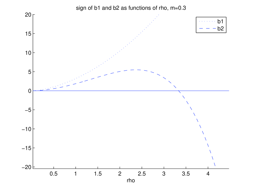
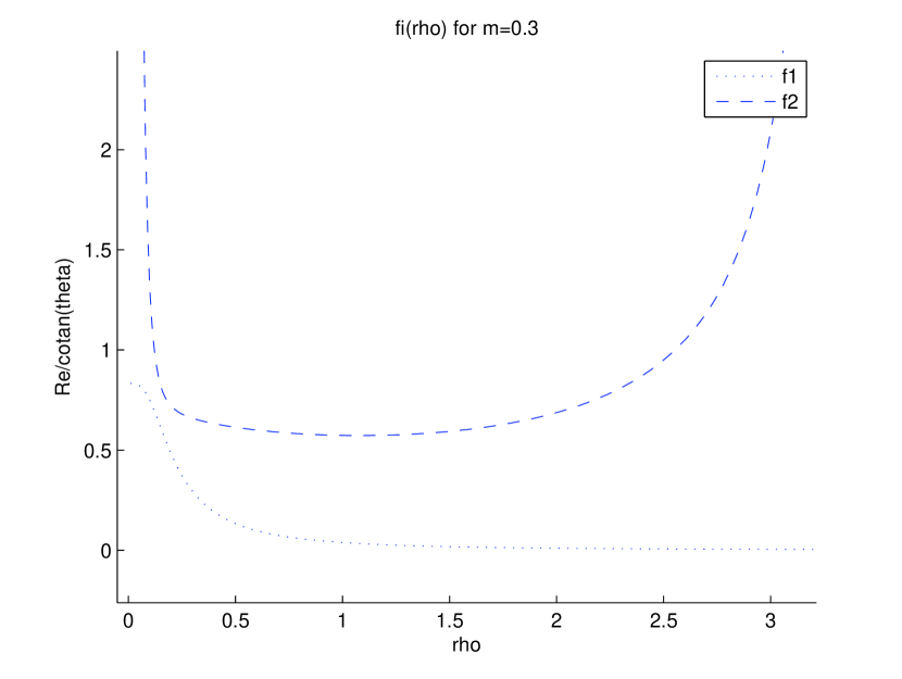
Figure 2: Values of $b_{i},i=1,2$ and the critical curves $\displaystyle f_{i}(\rho)=\frac{R_{e}}{{\rm cotan}\theta}$ for $\nu=0.3$

Let us consider the superposition of two incompressible and immiscible fluids with density, viscosity and capillarity $(\rho_{i},\nu_{i},\sigma_{i}),i=1,2$ flowing down an inclined plane with a slope $\theta$ (see figure 2).

Figure 1: Two fluids flowing down an inclined plane.

We introduce the aspect ratio $\varepsilon$, the Reynolds number $R_{e}$, the Froude number $F$ and Weber numbers $W_{i}$ as

$$\varepsilon=\frac{H}{L},\quad R_{e}=\frac{\rho_{1}HU}{\nu_{1}},\quad F^{2}=\frac{U^{2}}{gH},\quad W_{i}=\frac{\sigma_{i}}{\rho_{i}HU^{2}},\>i=1,2,$$

where $H$ denotes the characterictic depth of the fluid and $L$ the characteristic length in the streamwise direction. The characteristic fluid velocity $U$ can be chosen as the average velocity in the fluid layer for a Nusselt flow. We further introduce the additionnal numbers

$$\rho=\frac{\rho_{2}}{\rho_{1}},\quad\nu=\frac{\nu_{2}}{\nu_{1}}.$$

The motion of fluids (1) and (2) is described by Navier-Stokes equations

$$\displaystyle\varrho_{i}\big{(}\partial_{t}u_{i}+\partial_{x}u_{i}^{2}+\partial_{z}u_{i}w_{i}\big{)}+\frac{\partial_{x}p_{i}}{F^{2}} = \frac{s\varrho_{i}}{\varepsilon F^{2}}+\frac{\mu_{i}}{\varepsilon R_{e}}\big{(}\partial_{zz}u_{i}+\varepsilon^{2}\partial_{xx}u_{i}\big{)},$$ (1)

$$\displaystyle\varrho_{i}\big{(}\partial_{t}w_{i}+\partial_{x}u_{i}w_{i}+\partial_{z}w_{i}^{2}\big{)}+\frac{\partial_{z}p_{i}}{\varepsilon^{2}F^{2}} = -\frac{\varrho_{i}c}{\varepsilon^{2}F^{2}}+\frac{\mu_{i}}{\varepsilon R_{e}}\big{(}\partial_{zz}w_{i}+\varepsilon^{2}\partial_{xx}w_{i}\big{)},$$ (2)

$$\displaystyle\partial_{x}u_{i}+\partial_{z}w_{i} = 0,\quad i=1,2.$$ (3)

Here $\varrho_{1}=1$, $\varrho_{2}=\rho$, $\mu_{1}=1$, $\mu_{2}=\nu$. These equations are set in the fluid domains

$$\Omega_{1,t}=\left\{(x,z)\in\mathbb{R}^{2}/0\leq z\leq h_{1}(x,t)\right\}$$

and

$$\Omega_{2,t}=\left\{(x,z)\in\mathbb{R}^{2}/h_{1}(x,t)\leq z\leq h_{1}+h_{2}(x,t)=h(x,t)\right\}.$$

The kinematic conditions at the bottom, fluids interface and free surface are respectively

$$\begin{array}[]{lll}\displaystyle u_{1}(0,x)=w_{1}(0,x)=0,\quad u_{1}(h_{1})=u_{2}(h_{1}),\quad w_{1}(h_{1})=w_{2}(h_{1}),\\ \\ \displaystyle\partial_{t}h_{1}+u_{1}(h_{1})\partial_{x}h_{1}=w_{1}(h_{1}),\quad\partial_{t}h+u_{2}(h)\partial_{x}(h)=w_{2}(h).\end{array}$$ (4)

We assume the continuity of the fluid stress at the fluids interface and at the free surface. First, the continuity of normal stresses yields

$$\displaystyle p_{2}(h) = -\frac{\kappa_{2}\,F^{2}\partial_{xx}h}{\big{(}1+\varepsilon^{2}(\partial_{x}h)^{2}\big{)}^{\frac{3}{2}}}-\frac{2\nu\varepsilon F^{2}}{R_{e}}\partial_{x}u_{2}(h)\frac{1+\varepsilon^{2}(\partial_{x}h)^{2}}{1-\varepsilon^{2}(\partial_{x}h)^{2}},$$

$$\displaystyle p_{1}(h_{1})-p_{2}(h_{1}) = -\frac{\kappa_{1}\,F^{2}\partial_{xx}h_{1}}{\big{(}1+\varepsilon^{2}(\partial_{x}h_{1})^{2}\big{)}^{\frac{3}{2}}}$$

$$-\frac{2\varepsilon F^{2}}{Re}\big{(}\partial_{x}u_{1}(h_{1})-\nu\partial_{x}u_{2}(h_{1})\big{)}\frac{1+\varepsilon^{2}(\partial_{x}h_{1})^{2}}{1-\varepsilon^{2}(\partial_{x}h_{1})^{2}},$$

with $\kappa_{i}=\varepsilon^{2}\,W_{i}$. In order to take into account of the surface tension effects, we assume $\kappa_{i}=\mathcal{O}(1)$. Next, the continuity of tangential stresses yields

$$\displaystyle\big{(}\partial_{z}u_{2} + \varepsilon^{2}\partial_{x}w_{2}\big{)}(h)=4\varepsilon^{2}\frac{\partial_{x}u_{2}(h)}{1-\varepsilon^{2}\big{(}\partial_{x}h\big{)}^{2}}\partial_{x}h,$$

$$\displaystyle\nu\big{(}\partial_{z}u_{2} + \varepsilon^{2}\partial_{x}w_{2}\big{)}(h_{1})-\big{(}\partial_{z}u_{1}+\varepsilon^{2}\partial_{x}w_{1}\big{)}(h_{1})=4\varepsilon^{2}\frac{\big{(}\nu\partial_{x}u_{2}-\partial_{x}u_{1}\big{)}(h_{1})}{1-\varepsilon^{2}(\partial_{x}h_{1})^{2}}\partial_{x}h_{1}.$$

Let us now describe the stationary solutions of this system. The velocity field does not depend on $x$ and $t$. The fluid heights are constant $h_{1}(x,t)=\overline{h}$, $h_{2}(x,t)=1-\overline{h}$ whereas the pressure is hydrostatic

$$p_{1}(z)=c(\overline{h}-z)+\rho c(1-\overline{h}),\>\>\forall 0\leq z\leq\overline{h},\quad p_{2}(z)=\rho c(1-z),$$

and the fluid velocities have a parabolic profile

$$\begin{array}[]{ll}\displaystyle u_{1}(z)=\lambda\big{(}\rho(1-\overline{h})z+\overline{h}z-\frac{z^{2}}{2}\big{)},\quad\forall 0\leq z\leq\overline{h},\\ \displaystyle u_{2}(z)=\lambda\overline{h}(\rho(1-\overline{h})+\frac{\overline{h}}{2})+\frac{\lambda\rho}{\nu}\Big{(}(1-\overline{h})(z-\overline{h})-\frac{(z-\overline{h})^{2}}{2}\Big{)},\quad\forall\overline{h}\leq z\leq 1,\end{array}$$

where $\lambda$ is a constant defined as $\displaystyle\lambda=\frac{Re\sin\theta}{F^{2}}$.

In what follows, we will analyse the bi-layer flows in the neighbourhood of such steady solutions: this yields a natural scale for the characteristic fluid velocity $U$ and thus the constant $\lambda$ has to satisfy an extra relation. If one choose the ratio between the total mass discharge rate and the total mass of the fluid then

$$\begin{array}[]{ll}\displaystyle\int_{0}^{\overline{h}}u_{1}+\rho\int_{\overline{h}}^{1}u_{2}=\overline{h}+\rho(1-\overline{h}),\\ \displaystyle\lambda=3\frac{\overline{h}+\rho(1-\overline{h})}{\displaystyle\overline{h}^{3}+3\rho\overline{h}^{2}(1-\overline{h})+3\rho^{2}\overline{h}(1-\overline{h})^{2}+\frac{\rho^{2}}{\nu}(1-\overline{h})^{3}}.\end{array}$$

Note that for a single layer of fluid ($\rho=\nu=1$), one recovers the condition of Vila $\lambda=3$. Another possible choice for the characteristic velocity would be the fluid velocity at the free surface: one then recovers the classical value $\lambda=2$. In both cases, there is a relation between the Reynolds and Froude numbers. Here, we have chosen $U$ so that $\lambda=3$: there remains $R_{e}$, $\theta$, $\overline{h}$, $\kappa_{i}$, $\rho,\nu$ as free parameters to design an experiment and describe a bi-layer flow of Newtonian fluids.

We will derive shallow water equations from Navier Stokes equations integrated across each fluid layer (see e.g. [18], [16], [7]). First, we integrate the divergence free conditions on each fluid layer: using the kinematic conditions (4), we find the mass conservation laws:

$$\partial_{t}h_{1}+\partial_{x}\big{(}\int_{0}^{h_{1}}u_{1}(z)dz\big{)}=0,\quad\partial_{t}h_{2}+\partial_{x}\big{(}\int_{h_{1}}^{h}u_{2}(z)dz\big{)}=0.$$

Denote $q_{1}=h_{1}\overline{u}_{1}=\int_{0}^{h_{1}}u_{1}$ and $q_{2}=h_{2}\overline{u}_{2}=\int_{h_{1}}^{h}u_{2}$ the discharge rates in the streamwise direction: the mass conservation laws then read

$$\partial_{t}h_{1}+\partial_{x}(h_{1}\overline{u}_{1})=0,\quad\partial_{t}h_{2}+\partial_{x}(h_{2}\overline{u}_{2})=0.$$ (5)

Now, we write a system of equations which governs the evolution of $q_{i}=h_{i}\overline{u}_{i}$. This is done through the integration of momentum equations across each fluid layer:

$$\displaystyle\partial_{t}\big{(}\int_{0}^{h_{1}}u_{1}\big{)}+\partial_{x}\Big{(}\int_{0}^{h_{1}}u_{1}^{2} + \frac{p_{1}}{F^{2}}\Big{)}+\frac{\kappa_{1}\partial_{x}h_{1}\partial_{xx}h_{1}}{\big{(}1+\varepsilon^{2}(\partial_{x}h_{1})^{2}\big{)}^{\frac{3}{2}}}=-\frac{\partial_{z}u_{1}(0)}{\varepsilon R_{e}}$$

$$\frac{\lambda}{\varepsilon R_{e}}h_{1}+\frac{2\varepsilon}{R_{e}}\partial_{x}\Big{(}\int_{0}^{h_{1}}\partial_{x}u_{1}\Big{)}-\mathcal{T}$$

$$\displaystyle\partial_{t}\big{(}\rho\int_{h_{1}}^{h}u_{2}\big{)}+\partial_{x}\Big{(}\int_{h_{1}}^{h}\rho\,u_{2}^{2} + \frac{p_{2}}{F^{2}}\Big{)}+\frac{\kappa_{2}\partial_{x}h\partial_{xx}h}{\big{(}1+\varepsilon^{2}(\partial_{x}h)^{2}\big{)}^{\frac{3}{2}}}=$$ (6)

$$\frac{\lambda\rho h_{2}}{\varepsilon R_{e}}+\frac{2\varepsilon}{R_{e}}\partial_{x}\Big{(}\int_{h_{1}}^{h}\partial_{x}u_{2}\Big{)}+\mathcal{T},$$

with $\mathcal{T}$ defined as

$$\mathcal{T}=-\frac{p_{2}(h_{1})\partial_{x}h_{1}}{F^{2}}-\frac{\nu}{\varepsilon R_{e}}\partial_{z}u_{2}(h_{1})+\frac{\nu\varepsilon}{R_{e}}\big{(}2\partial_{x}u_{2}(h_{1})\partial_{x}h_{1}-\partial_{x}w_{2}(h_{1})\big{)}.$$

In order to write this evolution system in a closed form, one has to find a relation between the different integrated quantities, the tangential stresses at the wall, at the fluids interface, $\mathcal{T}$ and the unknowns $h_{i},q_{i}$. We follow the method introduced by Vila [19] in the case of a single fluid layer. We expand the velocity field with respect to $\varepsilon$ in order to find an expansion of the above quantities and $q_{i}$ as functions of $h_{i}$ and their derivatives to any fixed order. For a given order, this enables us to write the unknown quantities in system (2.1.1) as functions of $(h_{i},q_{i})$ and derive a shallow water model in a closed form.

2.1.2 Asymptotic expansions of solutions to Navier-Stokes eqs

In the shallow water regime $\varepsilon\approx 0$, the fluid velocities and pressures $u_{i},w_{i},p_{i}$ almost satisfy a differential system in $z$. The “horizontal” fluid velocities $u_{i},i=1,2$ are solution to:

$$\mu_{i}\partial_{zz}u_{i}+\varrho_{i}\lambda=\varepsilon R_{e}\varrho_{i}\big{(}\partial_{t}u_{i}+u_{i}\partial_{x}u_{i}+w_{i}\partial_{z}u_{i}\big{)}+\frac{\varepsilon R_{e}}{F^{2}}\partial_{x}p_{i}-\mu_{i}\varepsilon^{2}\partial_{xx}u_{i}.$$ (7)

We add the boundary conditions:

$$\displaystyle\partial_{z}u_{2}(h) = 4\varepsilon^{2}\frac{\partial_{x}u_{2}(h)}{1-\varepsilon^{2}\big{(}\partial_{x}h\big{)}^{2}}\partial_{x}h-\varepsilon^{2}\partial_{x}w_{2}(h),$$

$$\displaystyle\nu\partial_{z}u_{2}(h_{1})-\partial_{z}u_{1}(h_{1}) = 4\varepsilon^{2}\frac{\big{(}\nu\partial_{x}u_{2}-\partial_{x}u_{1}\big{)}(h_{1})}{1-\varepsilon^{2}(\partial_{x}h_{1})^{2}}\partial_{x}h_{1}$$

$$-\varepsilon^{2}\big{(}\nu\partial_{x}w_{2}(h_{1})-\partial_{x}w_{1}(h_{1})\big{)},$$

and $\displaystyle u_{1}(0)=0,\quad u_{1}(h_{1})=u_{2}(h_{1})$.

The fluid pressures are solutions to the differential system

$$\partial_{z}p_{i}+\varrho_{i}c=\mu_{i}\frac{\varepsilon F^{2}}{R_{e}}\partial_{zz}w_{i}-\varepsilon^{2}F^{2}\varrho_{i}\Big{(}\partial_{t}w_{i}+u_{i}\partial_{x}w_{i}+w_{i}\partial_{z}w_{i}\Big{)}+\mu_{i}\frac{\varepsilon^{3}F^{2}}{Re}\partial_{xx}w_{i},$$ (8)

whereas the boundary conditions for this system are given by

$$\displaystyle p_{2}(h) = -\frac{\kappa_{2}\,F^{2}\partial_{xx}h}{\big{(}1+\varepsilon^{2}(\partial_{x}h)^{2}\big{)}^{\frac{3}{2}}}-\frac{2\nu\varepsilon F^{2}}{R_{e}}\partial_{x}u_{2}(h)\frac{1+\varepsilon^{2}(\partial_{x}h)^{2}}{1-\varepsilon^{2}(\partial_{x}h)^{2}},$$

$$\displaystyle p_{1}(h_{1})-p_{2}(h_{1}) = -\frac{\kappa_{1}\,F^{2}\partial_{xx}h_{1}}{\big{(}1+\varepsilon^{2}(\partial_{x}h_{1})^{2}\big{)}^{\frac{3}{2}}}$$

$$-\frac{2\varepsilon F^{2}}{Re}\big{(}\partial_{x}u_{1}(h_{1})-\nu\partial_{x}u_{2}(h_{1})\big{)}\frac{1+\varepsilon^{2}(\partial_{x}h_{1})^{2}}{1-\varepsilon^{2}(\partial_{x}h_{1})^{2}},$$

Finally, the vertical velocities are solutions to

$$\partial_{z}w_{i}=-\partial_{x}u_{i},\quad w_{1}(0)=0,\quad w_{1}(h_{1})=w_{2}(h_{1}).$$

There are three nondimensional numbers that are relevant to parametrize this set of equations: let us define

$$\alpha=\frac{\varepsilon F^{2}}{R_{e}},\quad\beta=\varepsilon R_{e},\quad\delta=\frac{\varepsilon R_{e}}{F^{2}}.$$ (9)

In what follows, we will assume that $\alpha,\beta,\delta\ll 1$ so as to remain close to Nusselt type solutions. These assumptions are clearly satisfied when $R_{e},F=O(1)$ but a wider ranger of parameters is valid. Next, we compute an Hilbert expansion of the fluid velocity and pressure:

$$u_{i}=\sum_{k=0}^{\infty}u_{i}^{(k)},\quad p_{i}=\sum_{k=0}^{\infty}p_{i}^{(k)},$$

so that

$$u_{i}-\sum_{k=0}^{j}u_{i}^{(k)}=\mathcal{O}\Big{(}(\alpha+\beta+\delta)^{j+1}\Big{)},\quad p_{i}-\sum_{k=0}^{j}p_{i}^{(k)}=\mathcal{O}\Big{(}(\alpha+\beta+\delta)^{j+1}\Big{)}.$$

Let us first compute $u_{i}^{(0)},p_{i}^{(0)}$ Letting $\alpha,\beta,\delta\to 0$ in the above equations leads a differential system in the $z$ variable that is similar to the one which determines stationary solutions. The fluid pressure is (up to this order) hydrostatic:

$$\begin{array}[]{ll}\displaystyle p_{1}^{(0)}(z)=c(\rho h_{2}+h_{1}-z)-\kappa_{1}F^{2}\partial_{xx}h_{1}-\kappa_{2}F^{2}\partial_{xx}h,\\ \displaystyle p_{2}^{(0)}(z)=\rho c(h_{1}+h_{2}-z)-\kappa_{2}F^{2}\partial_{xx}h.\end{array}$$ (10)

The fluid velocities in the streamwise direction have a parabolic profile

$$\begin{array}[]{ll}\displaystyle u_{1}^{(0)}(z)=\lambda\big{(}\rho h_{2}z+h_{1}z-\frac{z^{2}}{2}\big{)},\\ \displaystyle u_{2}^{(0)}(z)=\lambda h_{1}\big{(}\rho h_{2}+\frac{h_{1}}{2}\big{)}+\frac{\lambda\rho}{\nu}\big{(}h_{2}(z-h_{1})-\frac{(z-h_{1})^{2}}{2}\big{)}.\end{array}$$ (11)

The computation of higher order terms is then straightforward: assume that we have computed $u_{i}^{(j)},p_{i}^{(j)},\;j\leq k$, then $u_{i}^{(k+1)}$ is calculated by computing the solution to

$$\mu_{i}\partial_{zz}u_{i}^{(k+1)}=F_{i,k}(u_{n}^{(j)},p_{n}^{(j)}),\quad j\leq k,\quad n=1,2$$ (12)

with the boundary conditions

$$\begin{array}[]{ll}\displaystyle\partial_{z}u_{2}^{(k+1)}(h_{1}+h_{2})=g_{2}^{(k)},\quad\nu\partial_{z}u_{2}^{(k+1)}(h_{1})-\partial_{z}u_{1}^{(k+1)}(h_{1})=g_{1}^{(k)},\\ \displaystyle u_{1}^{(k+1)}(h_{1})=u_{2}^{(k+1)}(h_{1}),\quad u_{1}^{(k+1)}(0)=0.\end{array}$$ (13)

The solution $u_{i}^{(k+1)}$ to this system is

$$\displaystyle u_{1}^{(k+1)} = z\Big{(}\nu\,g_{2}^{(k)}-g_{1}^{(k)}-\int_{h_{1}}^{h}F_{2,k}(y)dy\Big{)}-\int_{0}^{z}\int_{\overline{z}}{h_{1}}F_{1,k}(y)dy\,d\overline{z},$$

$$\displaystyle u_{2}^{(k+1)} = h_{1}\Big{(}\nu\,g_{2}^{(k)}-g_{1}^{(k)}-\int_{h_{1}}^{h}F_{2,k}(y)dy\Big{)}-\int_{0}^{h_{1}}\int_{\overline{z}}^{h_{1}}F_{1,k}(y)dyd\overline{z}$$

$$+ g_{2}^{(k)}(z-h_{1})-\frac{1}{\nu}\int_{h_{1}}^{z}\int_{\overline{z}}^{h}F_{2,k}(y)dyd\overline{z}.$$

We determine similarly an expansion of the fluid pressure to any fixed order.

2.2 Lubrication theory

The fluid velocities and pressures are expanded with respect to $\alpha,\beta,\delta\ll 1$, $h_{i}$ and their space and time derivatives: we use zeroth and first order expansions of $u_{i}$ to obtain respectively inviscid and viscous conservation laws for $h_{1},h_{2}$. Then we study the spectral stability of steady states.

2.2.1 Inviscid and viscous conservation laws

We first compute an inviscid system of conservation laws, which is the analogous of Burgers equations in the case of a single fluid layer. The fluids velocities are given by $\displaystyle u_{i}=u_{i}^{(0)}+\mathcal{O}(\alpha+\beta+\delta)$. The discharge rates $q_{i},i=1,2$ are expanded as

$$\begin{array}[]{ll}\displaystyle q_{1}=\int_{0}^{h_{1}}u_{1}=\lambda h_{1}^{2}\Big{(}\frac{\rho h_{2}}{2}+\frac{h_{1}}{3}\Big{)}+\mathcal{O}(\alpha+\beta+\delta),\\ \displaystyle q_{2}=\int_{h_{1}}^{h}u_{2}=\lambda h_{1}h_{2}(\rho h_{2}+\frac{h_{1}}{2})+\frac{\lambda\rho}{\nu}\frac{h_{2}^{3}}{3}.+\mathcal{O}(\alpha+\beta+\delta).\end{array}$$ (14)

Inserting (14) into the mass conservation laws (5) yields

$$\begin{array}[]{ll}\displaystyle\partial_{t}h_{1}+\partial_{x}\Big{(}\lambda h_{1}^{2}\big{(}\frac{\rho h_{2}}{2}+\frac{h_{1}}{3}\big{)}\Big{)}=\mathcal{O}(\alpha+\beta+\delta),\\ \displaystyle\partial_{t}h_{2}+\partial_{x}\Big{(}\lambda h_{1}h_{2}\big{(}\rho h_{2}+\frac{h_{1}}{2}\big{)}+\frac{\lambda\rho}{\nu}\frac{h_{2}^{3}}{3}\Big{)}=\mathcal{O}(\alpha+\beta+\delta).\end{array}$$ (15)

We drop $\mathcal{O}(\alpha+\beta+\delta)$ terms in (15) and obtain a system of partial differential equations for $(h_{1},h_{2})$ in a closed form. A necessary condition of stability of steady state is that (15) is a hyperbolic system. When this condition is satisfied, we obtain a useful information on the group velocities $\Lambda_{+}>\Lambda_{-}$ of low frequency perturbations (respectively the velocities at the free surface and at the fluid interface):

$$\displaystyle\Lambda_{\pm} = \frac{\lambda}{4\nu}\big{(}2\rho h_{2}^{2}+6\rho\nu h_{1}h_{2}+3\nu h_{1}^{2}\pm\sqrt{\Delta}\big{)}$$

$$\displaystyle\Delta = \left(h_{1}^{2}\left(2\rho h_{2}+h_{1}\right)+8\rho^{2}h_{1}^{2}h_{2}^{2}\right)\nu^{2}+4\rho h_{1}h_{2}^{2}\left(2\rho h_{2}-h_{1}\right)\nu+4\rho^{2}h_{2}^{4}$$

Strict hyperbolicity is ensured if and only if $\Delta>0$. As it is a quadratic form in $\nu$ the discriminant of $\Delta$ is $-128\rho^{3}h_{1}^{2}h_{2}^{5}\left(h_{1}+\rho h_{2}\right)$, which is negative when $h_{1}$, $h_{2}$, $\rho$ are strictly positive. Then $h_{1}>0$ and $h_{2}>0$ ensure that the system (15) is strictly hyperbolic.

Next, we use first order expansions of fluid velocities

$$u_{i}=u_{i}^{(0)}+u_{i}^{(1)}+\mathcal{O}\big{(}(\alpha+\beta+\delta)^{2}\big{)}$$

to determine a more accurate system of equations. Inserting the expansion of $q_{i},i=1,2$ into the mass conservation laws yields a system of Benney’s equations (or Kuramoto-Sivashinsky when surface tension is considered)

$$\displaystyle\partial_{t}\left(\begin{array}[]{c}h_{1}\\ h_{2}\end{array}\right)+\partial_{x}\left(\begin{array}[]{c}\displaystyle\lambda h_{1}^{2}(\frac{h_{1}}{3}+\frac{\rho h_{2}}{2})\\ \displaystyle\lambda h_{1}h_{2}(\rho h_{2}+\frac{h_{1}}{2})+\frac{\lambda\rho}{3\nu}h_{2}^{3}\end{array}\right) = \lambda\beta\partial_{x}\Big{(}d(h_{i})\partial_{x}\left(\begin{array}[]{c}h_{1}\\ h_{2}\end{array}\right)\Big{)}$$ (22)

$$+ \beta\partial_{x}\Big{(}K(h_{i})\partial_{x}^{3}\left(\begin{array}[]{c}h_{1}\\ h_{2}\end{array}\right)\Big{)},$$ (25)

with the viscous coefficients $d_{i,j}$ defined as $\displaystyle d_{i,j}=\frac{\cot\theta}{R_{e}}d_{i,j,1}-\lambda\,d_{i,j,2}$

$$\displaystyle d_{1,1,1} = h_{1}^{2}(\frac{h_{1}}{3}+\frac{\rho h_{2}}{2}),\quad d_{1,2,1}=\rho h_{1}^{2}(\frac{h_{1}}{3}+\frac{h_{2}}{2}),$$

$$\displaystyle d_{2,1,1} = \frac{\rho h_{2}^{3}}{3\nu}+\rho h_{1}h_{2}^{2}+h_{2}\frac{h_{1}^{2}}{2},\quad d_{2,2,1}=\frac{\rho h_{2}^{3}}{3\nu}+\rho h_{1}h_{2}^{2}+\rho h_{2}\frac{h_{1}^{2}}{2},$$

$$\displaystyle d_{1,1,2} = \frac{h_{1}^{2}}{\nu}\Big{(}\frac{2h_{1}^{4}}{15}+\frac{71\rho\nu}{120}h_{1}^{3}h_{2}+\frac{23\rho^{2}\nu}{24}h_{1}^{2}h_{2}^{2}+(\frac{\rho^{2}}{6}+\frac{\rho^{2}\nu}{2})h_{1}h_{2}^{3}+\frac{\rho^{3}}{6}h_{2}^{4}\Big{)},$$

$$\displaystyle d_{1,2,2} = \frac{\rho h_{1}^{2}}{\nu^{2}}\Big{(}\frac{2\nu^{2}h_{1}^{4}}{15}+\frac{71\rho\nu^{2}}{120}h_{1}^{3}h_{2}+(\frac{5\rho\nu}{24}+\frac{3\rho^{2}\nu^{2}}{4})h_{1}^{2}h_{2}^{2}+\frac{2\rho^{2}\nu}{3}h_{1}h_{2}^{3}+\frac{\rho^{2}}{6}h_{2}^{4}\Big{)},$$

$$\displaystyle d_{2,1,2} = \frac{h_{2}}{\nu^{2}}\Big{(}\frac{5\nu^{2}h_{1}^{5}}{24}+\frac{25\rho\nu^{2}}{24}h_{1}^{4}h_{2}+(\frac{11\rho^{2}\nu^{2}}{6}+\frac{\rho\nu}{6})h_{1}^{3}h_{2}^{2}$$

$$+(\rho^{3}\nu^{2}+\frac{5\rho^{2}\nu}{6})h_{1}^{2}h_{2}^{3}+(\frac{2\rho^{2}}{15}+\frac{2\rho^{3}\nu}{3})h_{1}h_{2}^{4}+\frac{2\rho^{3}}{15}h_{2}^{5}\Big{)},$$

$$\displaystyle d_{2,2,2} = \frac{\rho h_{2}}{\nu^{2}}\Big{(}\frac{5\nu^{3}}{24}h_{1}^{5}+\frac{25\rho\nu^{3}}{24}h_{1}^{4}h_{2}+(\frac{3\rho^{2}\nu^{3}}{2}+\frac{\rho\nu^{2}}{2})h_{1}^{3}h_{2}^{2}$$ (26)

$$+\frac{11\rho^{2}\nu^{2}}{6}h_{1}^{2}h_{2}^{3}+\frac{4\rho^{2}\nu h_{1}h_{2}^{4}}{5}+\frac{2\rho^{2}}{15}h_{2}^{5}\Big{)}.$$

The surface tension terms are given by

$$\begin{array}[]{lll}\displaystyle K_{1,1}=h_{1}^{2}\big{(}(\kappa_{1}+\kappa_{2})\frac{h_{1}}{3}+\kappa_{2}\frac{h_{2}}{2}\big{)},\quad K_{1,2}=\kappa_{2}\,h_{1}^{2}\big{(}\frac{h_{1}}{3}+\frac{h_{2}}{2}\big{)},\\ \displaystyle K_{2,1}=\frac{\kappa_{2}h_{2}^{3}}{3\nu}+\kappa_{2}h_{2}^{2}h_{1}+(\kappa_{1}+\kappa_{2})\frac{h_{2}h_{1}^{2}}{2},\\ \displaystyle K_{2,2}=\frac{\kappa_{2}h_{2}^{3}}{3\nu}+\kappa_{2}h_{1}h_{2}^{2}+\frac{\kappa_{2}h_{2}h_{1}^{2}}{2}.\end{array}$$ (27)

This system is in agreement with the one in [11]. In the low frequency regime, the system (22) of viscous conservation laws provides a criterion of spectral stability for the steady solutions which is consistent with the one given by Orr-Sommerfeld equations (if $R_{e},F=O(1)$). One goal of this paper is to study the formation of roll-waves in bi-layer flows. In the single layer case, they are the result ofthe competition between buoyancy and inertia. Therefore, we focus on the competition between inertia and buoyancy and their interaction with convective terms to describe the onset of roll-waves.

2.2.2 Spectral Stability of Steady States

Let us linearise (22) at a constant state $(\overline{h}_{1},\overline{h}_{2})$:

$$\partial_{t}\left(\begin{array}[]{c}h_{1}\\ h_{2}\end{array}\right)+J(\overline{h}_{i})\partial_{x}\left(\begin{array}[]{c}h_{1}\\ h_{2}\end{array}\right)=\lambda\beta d(\overline{h}_{i})\partial_{xx}\left(\begin{array}[]{c}h_{1}\\ h_{2}\end{array}\right).$$ (28)

Without loss of generality, we assume $\lambda\beta=1$. We have neglected the contribution of surface tension as they are not relevant in the low frequency regime. The dispersion relation is given by

$${\rm det}(\Lambda Id+ik\,J(h)+k^{2}\,d(h))=0,\quad\forall\,k\in\mathbb{R}.$$ (29)

and we assume $|k|\ll 1$. We expand $\Lambda_{j},j=1,2$ as $\Lambda_{j}=ik\tilde{\Lambda}_{j}$. Equation (29) then reads

$${\rm det}\big{(}\tilde{\Lambda}+J(\overline{h})\big{)}=ik{\rm tr}\Big{(}{\rm com}\big{(}\tilde{\Lambda}Id+J(\overline{h})\big{)}^{T}d(\overline{h})\Big{)}+\mathcal{O}(k^{2}).$$

System (15) is strictly hyperbolic : the eigenvalues $\overline{\Lambda}_{i}$ of $J(\overline{h})$ are real and $\overline{\Lambda}_{1}>\overline{\Lambda}_{2}$. Then $\Lambda_{1}(k),\Lambda_{2}(k)$ expand at $k=0$ as

$$\Lambda_{j}(k)=-ik\overline{\Lambda}_{j}-k^{2}\frac{{\rm tr}\Big{(}{\rm com}\big{(}J(\overline{h}_{i})-\overline{\Lambda}_{j}Id\big{)}^{T}d(\overline{h}_{i})\Big{)}}{{\rm tr}\big{(}J(\overline{h}_{i})\big{)}-2\overline{\Lambda}_{j}}+\mathcal{O}(k^{3}).$$ (30)

As a result, stationary solutions are stable if

$${\rm tr}\Big{(}{\rm com}\big{(}J(\overline{h})-\overline{\Lambda}_{1}Id\big{)}^{T}d(\overline{h})\Big{)}<0,\quad{\rm tr}\Big{(}{\rm com}\big{(}J(\overline{h})-\overline{\Lambda}_{2}Id\big{)}^{T}d(\overline{h})\Big{)}>0.$$ (31)

We consider two particular situations: stable and unstable density stratification: we will see that in some particular situations, the Rayleigh Taylor instability may be suppressed by the convection. We also study the influence of inertia on stability properties.

The spectral stability conditions (31) have the simple form

$$a_{1}(\rho)\frac{{\rm cotan}\theta}{R_{e}}<\lambda\,a_{2}(\rho),\quad b_{1}(\rho)\frac{{\rm cotan}\theta}{R_{e}}>\lambda\,b_{2}(\rho).$$

It is easily seen that $a_{i}<0$: the free surface is then stable if

$$R_{e}\leq\frac{a_{1}(\rho)}{\lambda a_{2}(\rho)}{\rm cotan}\theta.$$

The situation is more involved for the fluid interface where $b_{i}$ can change sign. If $b_{1}(\rho)b_{2}(\rho)<0$, the interface is stable when $b_{1}(\rho)>0$ and unstable otherwise. If $b_{1}(\rho)b_{2}(\rho)>0$, the fluid interface is stable if

$$b_{1}(\rho)\big{(}R_{e}-\frac{b_{1}(\rho)}{\lambda b_{2}(\rho)}{\rm cotan}\theta\big{)}<0.$$

In order to simplify the spectral analysis, we set $\overline{h}_{i}=1,i=1,2$ and consider the cases $\nu<1$, $\nu=1$ and $\nu>1$ (stratification in viscosity). We have determined stability curves $R_{e}=f_{k}(\rho){\rm cotan}\theta,k=1,2$ associated to the surface mode $k=1$ and the interfacial mode $k=2$.

Case 1: $\nu<1$. We have chosen here $\nu=0.3$, $\nu=0.7$ and $\nu=0.9$ that gives a good representation of all possible scenarii that arises as $\rho$ varies. Let us first check the case $\nu=0.3$. We have represented critical curves in picture 2.

There exists $\rho_{c}\approx 3.3$ above which $b_{2}<0$ otherwise both $b_{i}>0,i=1,2$. Then, for $\rho>\rho_{c}$, the interfacial mode is stable whereas the full system is spectrally stable if $\mathbb{R}_{e}<f_{1}(\rho){\rm cotan}\theta$. If $\rho<\rho_{c}$, $f_{1}(\rho)<f_{2}(\rho)$: if $R_{e}$ is sufficiently small, the flow is stable and as $R_{e}$ is increased, the surface mode is destabilized before the interfacial mode.

Next we consider the case $\nu=0.7$. The critical curves are represented in picture 3.

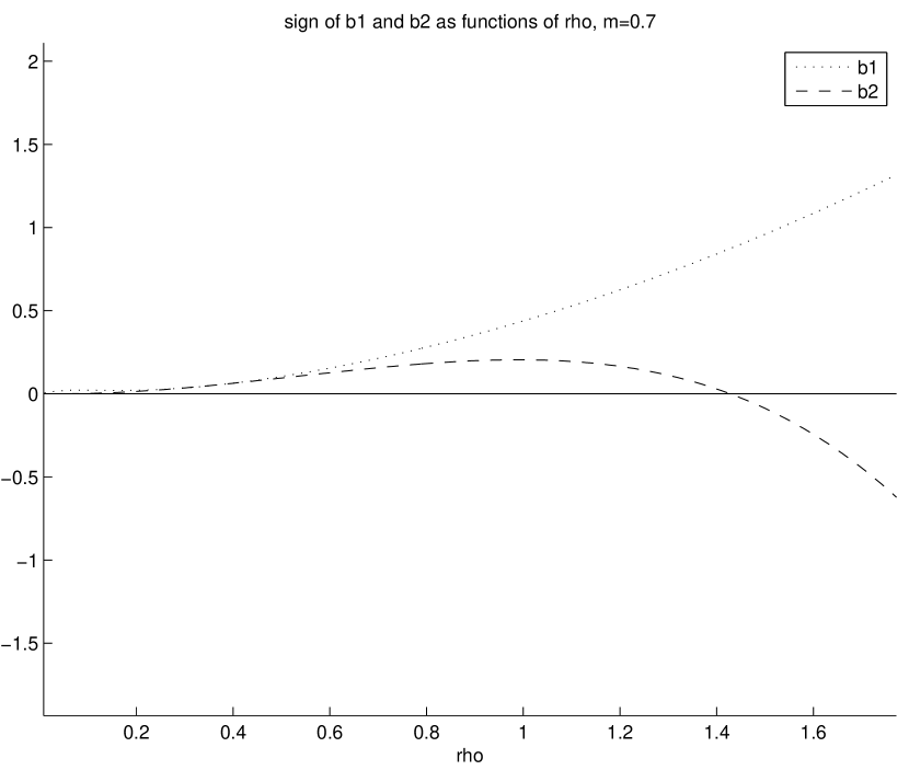
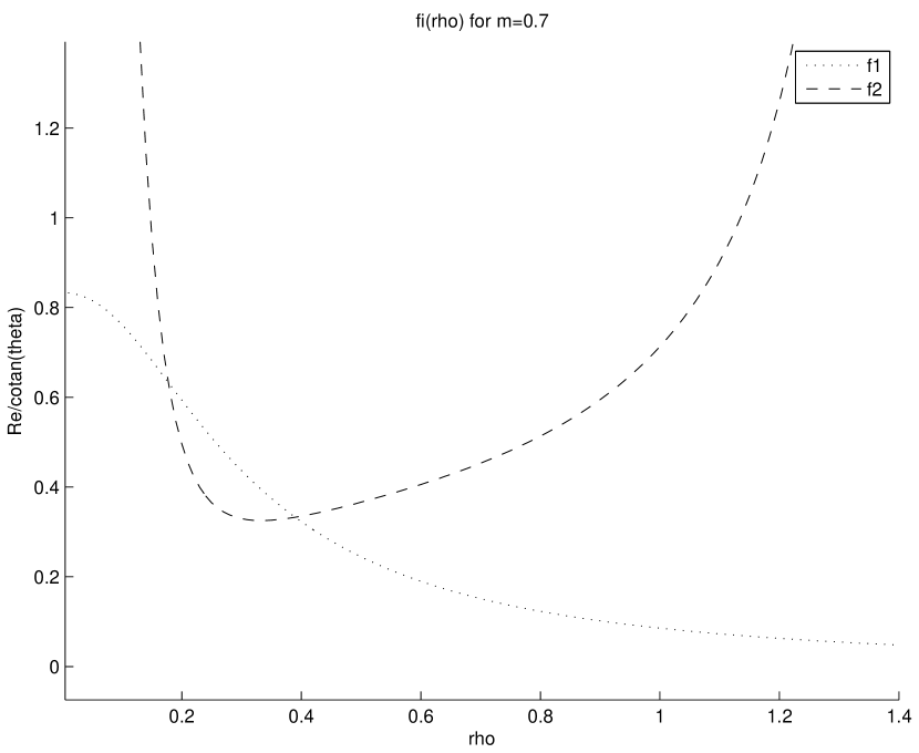
Figure 3: Values of $b_{i},i=1,2$ and the critical curves $\displaystyle f_{i}(\rho)=\frac{R_{e}}{{\rm cotan}\theta}$ for $\nu=0.7$

There exists $\rho_{c}\approx 1.4$ above which the interfacial mode is always unstable whereas the surface mode is stable for $R_{e}<f_{2}(\rho){\rm cotan}\theta$. If $\rho<\rho_{c}$, there exists $\rho_{1}<\rho_{2}$ so that for any $\rho<\rho_{1}$ or $\rho_{2}<\rho<\rho_{c}$, the scenario is identical to the previous case: as $R_{e}$ is increased, the surface mode is destabilized before the interface mode. If $\rho_{1}<\rho<\rho_{2}$, the interfacial mode is destabilized first as $R_{e}$ is increased. The case $\nu=0.9$ is similar, except that for $\rho_{1}<\rho<\rho_{2}$, the interfacial mode is always unstable (see picture 4).

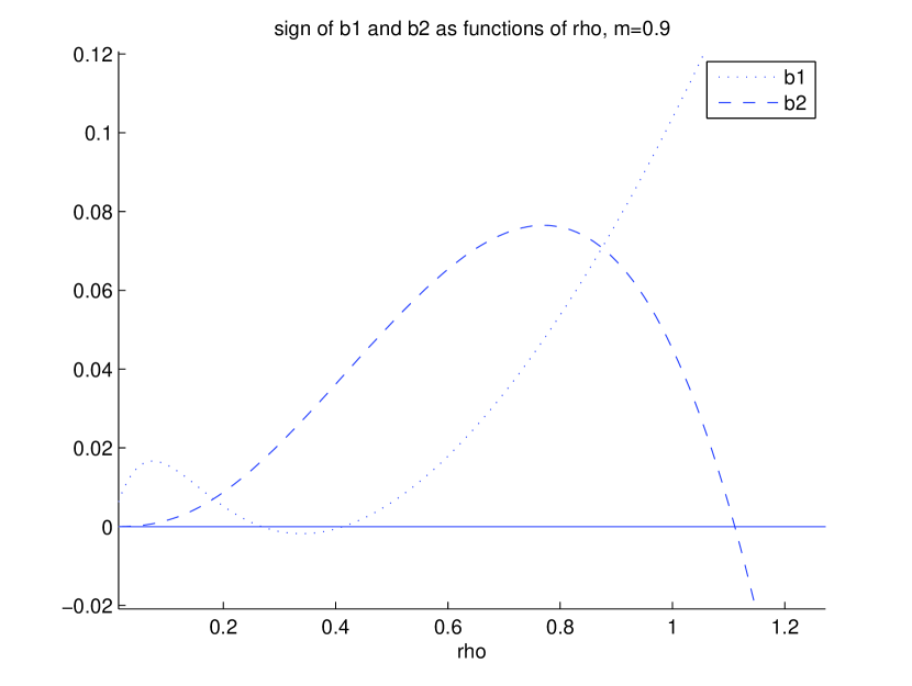
Figure 4: Values of $b_{i},i=1,2$ and the critical curves $\displaystyle f_{i}(\rho)=\frac{R_{e}}{{\rm cotan}\theta}$ for $\nu=0.9$

Case 2: $\nu=1$. There exists $\rho_{c}$ above which the interfacial mode is always stable. If $\rho<\rho_{c}$, there exists $\rho_{1}<\rho_{c}$ so that the interface mode is always unstable if $\rho_{1}<\rho<\rho_{c}$. If $\rho<\rho_{1}$, the surface mode is destablized first $R_{e}$ is increased (see figure 5).

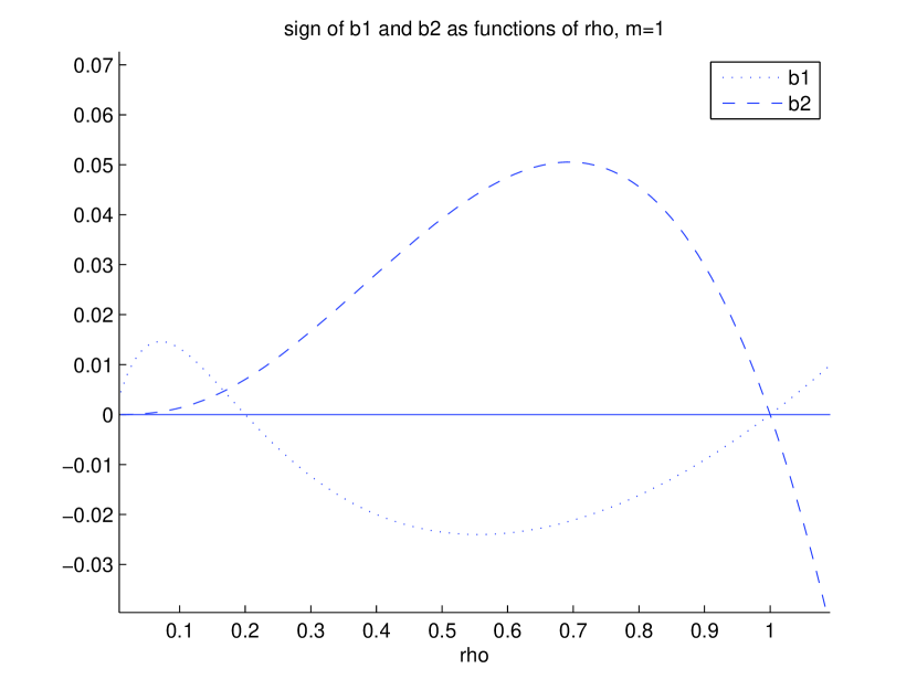
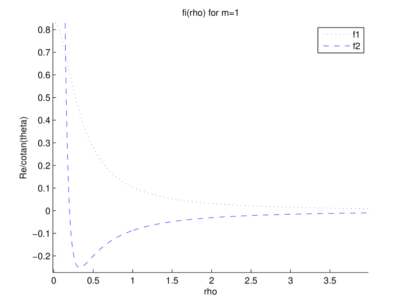
Figure 5: Values of $b_{i},i=1,2$ and the critical curves $\displaystyle f_{i}(\rho)=\frac{R_{e}}{{\rm cotan}\theta}$ for $\nu=1$

Case 3: $\nu>1$. We have chosen $\nu=1.1$ and $\nu=1.5$, which gives a good representation of all possible scenarii that arises as $\rho$ varies. We first consider $\nu=1.1$ (see figure 6).

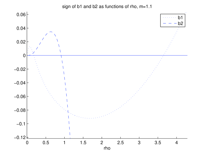
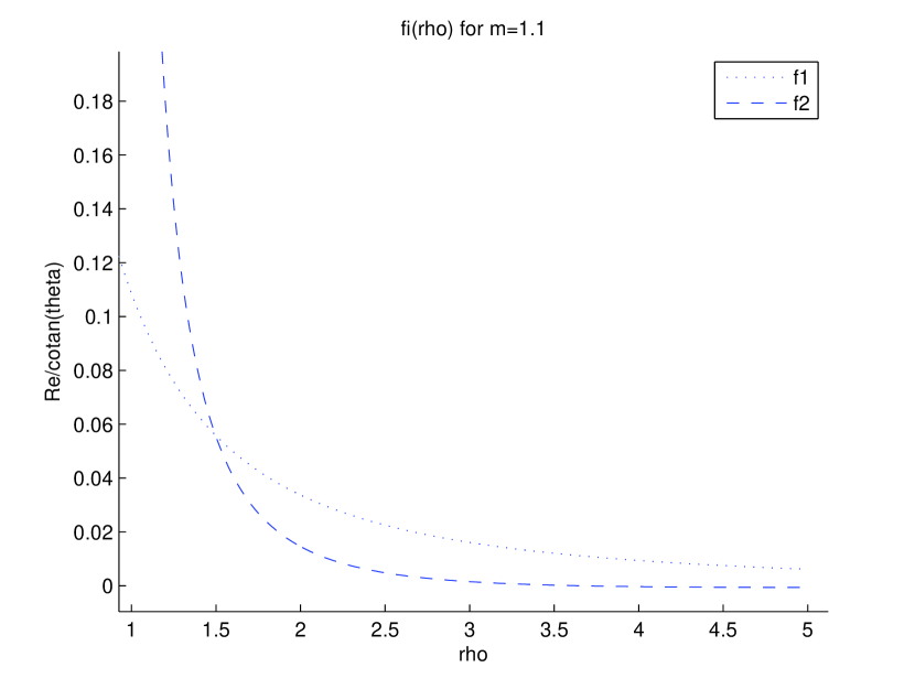
Figure 6: Values of $b_{i},i=1,2$ and the critical curves $\displaystyle f_{i}(\rho)=\frac{R_{e}}{{\rm cotan}\theta}$ for $\nu=1.1$

There exists $\rho_{c}\approx 3.5$ above which the interfacial mode is always stable. Assume $\rho<\rho_{c}$ and denote $\rho_{1}<\rho_{2}$ respectively the first zeros of $b_{1}$ and the zero of $b_{2}$. If $\rho_{1}<\rho<\rho_{2}$, the interfacial mode is always unstable and if $\rho<\rho_{1}$, the situation is similar to previous cases when $\rho$ is small. If $\rho>\rho_{2}$, the interfacial mode is stable only if $R_{e}>f_{1}(\rho){\rm cotan}\theta$. As a consequence, even at low Reynolds number, the interfacial mode is unstable. It is easily seen that there exists $\rho_{2}<\rho_{3}<\rho_{c}$ such that the flow is always unstable if $\rho_{2}<\rho<\rho_{3}$, stable if $\rho_{3}<\rho<\rho_{3}$ and

$$f_{2}(\rho){\rm cotan}\theta<R_{e}<f_{1}(\rho){\rm cotan}\theta.$$

Finally, we consider the case $\nu=1.5$ (see figure 7).

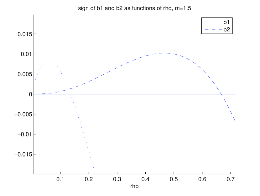
Figure 7: Values of $b_{i},i=1,2$ and the critical curves $\displaystyle f_{i}(\rho)=\frac{R_{e}}{{\rm cotan}\theta}$ for $\nu=1.5$

If $\rho_{1}$ is the zero of $b_{1}$, then for any $\rho>\rho_{1}$, the flow is always unstable under long wavelength perturbations. If $\rho<\rho_{1}$, the situation is similar to the cases $\nu<1$ when $\rho$ is stable: the flow is stable at low Reynolds number and the flow destabilizes first through the surface mode or the interfacial mode.

2.3 Shallow water theory

The viscous conservation laws which govern the evolution of $h_{i}$ are sufficient to obtain a consistent stability criterion of constant states in the low frequency regime. However, the solutions to this system blow up in finite time when the flow is unstable and may lead to some inaccuracy in the description of the motion of bi-layer flows. In what follows, we consider shallow water models: indeed in the case of a single fluid layer, they sustain nonlinear waves, so called “roll-waves” which are well known hydrodynamic instabilities. As a consequence, shallow water models are useful to describe the transition to instability in shallow flows. Up to our knowledge, there’s no consistent shallow water model which describes bi-layer flows down a ramp (the single layer case was treated only recently [16],[19]).

Let us keep $\mathcal{O}(1)$ and $\mathcal{O}(\varepsilon^{-1})$ terms in (2.1.1):

$$\displaystyle\partial_{t}\big{(}\int_{0}^{h_{1}}u_{1}\big{)}+\partial_{x}\Big{(}\int_{0}^{h_{1}}u_{1}^{2}+\frac{p_{1}}{F^{2}}\Big{)} + \kappa_{1}\partial_{x}h_{1}\partial_{xx}h_{1}=$$

$$\frac{1}{\varepsilon R_{e}}\big{(}\lambda h_{1} + \nu\partial_{z}u_{2}(h_{1})-\partial_{z}u_{1}(0)\big{)}+\frac{p_{2}(h_{1})\partial_{x}h_{1}}{F^{2}}$$

$$\displaystyle\partial_{t}\big{(}\rho\int_{h_{1}}^{h}u_{2}\big{)}+\partial_{x}\Big{(}\rho\int_{h_{1}}^{h}u_{2}^{2}+\frac{p_{2}}{F^{2}}\Big{)} + \kappa_{2}\partial_{x}h\partial_{xx}h=$$

$$\displaystyle\frac{1}{\varepsilon R_{e}}\big{(}\lambda\rho h_{2} - \nu\partial_{z}u_{2}(0)\big{)}-\frac{p_{2}(h_{1})\partial_{x}h_{1}}{F^{2}}.$$ (32)

We first compute an expansion of the integrals: the integrals of the pressures are given by

$$\begin{array}[]{lll}\displaystyle\int_{h_{i-1}}^{h_{i-1}+h_{i}}p_{i}=\int_{0}^{h_{1}}p_{i}^{(0)}+\mathcal{O}(\alpha+\beta+\delta),\quad i=1,2,\\ \displaystyle\int_{0}^{h_{1}}p_{1}^{(0)}=c\frac{h_{1}^{2}}{2}+\rho ch_{1}h_{2}-h_{1}F^{2}\big{(}(\kappa_{2}+\kappa_{1})\partial_{xx}h_{1}-\kappa_{2}\partial_{xx}h_{2}\big{)},\\ \displaystyle\int_{h_{1}}^{h}p_{2}^{(0)}=\rho c\frac{h_{2}^{2}}{2}-\kappa_{2}F^{2}h_{2}\partial_{xx}h_{2}.\end{array}$$ (33)

whereas the integrals of convection terms are given by

$$\displaystyle\int_{h_{i-1}}^{h_{i-1}+h_{i}}u_{i}^{2} = \int_{h_{i-1}}^{h_{i-1}+h_{i}}(u_{i}^{(0)})^{2}+\mathcal{O}(\alpha+\beta+\delta),\quad i=1,2$$

$$\displaystyle\int_{0}^{h_{1}}(u_{1}^{(0)})^{2} = \lambda^{2}h_{1}^{3}\Big{(}\frac{2}{15}h_{1}^{2}+\frac{5}{12}\rho h_{1}h_{2}+\frac{\rho^{2}h_{2}^{3}}{3}\Big{)},$$

$$\displaystyle\int_{h_{1}}^{h}(u_{2}^{(0)})^{2} = \lambda^{2}\big{(}\frac{2\rho^{2}}{15\nu^{2}}h_{2}^{5}+\frac{2\rho}{3\nu}(\rho h_{1}h_{2}+\frac{h_{1}^{2}}{2})h_{2}^{3}\big{)}$$

$$+\lambda^{2}\,h_{1}^{2}\big{(}\rho^{2}h_{2}^{3}+\rho h_{2}^{2}h_{1}+\frac{h_{2}h_{1}^{2}}{4})\big{)}.$$

In both cases, we only keep $O(1)$ terms. In order to write these quantities as classical convective terms, we introduce $Q_{i},i=1,2$ so that

$$\int_{0}^{h_{1}}(u_{1}^{(0)})^{2}=h_{1}\overline{u}_{1}^{2}+Q_{1}(h_{1},h_{2}),\quad\int_{h_{1}}^{h}(u_{2}^{(0)})^{2}=h_{2}\overline{u}_{2}^{2}+Q_{2}(h_{1},h_{2}).$$ (34)

Here, $Q_{i}$ depend on $h_{i}$ and are defined as

$$Q_{1}=\lambda^{2}\,h_{1}^{3}\Big{(}\frac{h_{1}^{2}}{45}+\frac{\rho h_{2}}{12}(h_{1}+\rho h_{2})\Big{)},\quad Q_{2}=\lambda^{2}\frac{\rho^{2}\,h_{2}^{5}}{45\,\nu^{2}}.$$

Inserting (33) and (2.3) into (2.3), one finds

$$\displaystyle\partial_{t}(h_{1}\overline{u}_{1})+\partial_{x}\Big{(}h_{1}\overline{u}_{1}^{2} + \frac{c}{F^{2}}\big{(}\rho h_{1}h_{2}+\frac{h_{1}^{2}}{2}\big{)}+Q_{1}\Big{)}-h_{1}\partial_{xxx}\big{(}\kappa_{2}(h_{1}+h_{2})+\kappa_{1}h_{1}\big{)}$$

$$= \frac{\rho c}{F^{2}}h_{2}\partial_{x}h_{1}+\frac{sh_{1}}{\varepsilon F^{2}}+\frac{1}{\varepsilon R_{e}}\big{(}\nu\partial_{z}u_{2}(h_{1})-\partial_{z}u_{1}(0)\big{)},$$

$$\displaystyle\rho\Big{(}\partial_{t}(h_{2}\overline{u}_{2})+\partial_{x}\big{(}h_{2}\overline{u}_{2}^{2} + \frac{c}{F^{2}}\frac{h_{2}^{2}}{2}+Q_{2}\big{)}\Big{)}-\kappa_{2}h_{2}\partial_{xxx}h$$

$$= -\frac{\rho c}{F^{2}}h_{2}\partial_{x}h_{1}+\frac{\rho s\,h_{2}}{\varepsilon F^{2}}-\frac{\nu}{\varepsilon R_{e}}\partial_{z}u_{2}(h_{1}).$$

This system is almost in a closed form. Let us now write $\partial_{z}u_{1}(0)$ and $\partial_{z}u_{2}(h_{1})$ as functions of $\overline{u}_{i}$ and $h_{i}$. We clearly see that an expansion of $u_{i}$ up to order $\mathcal{O}\big{(}(\alpha+\beta+\delta)^{2}\big{)}$ is needed. We use the method introduced by Vila [19] in the case of a single fluid layer to write these terms in a closed form. In [19], the wall stress is chosen proportionnal to the average velocity. One has to expand both the wall stress and the average velocity up to order $1$ and obtains an expansion of the wall stress with a zeroth order term proportionnal to the average velocity, the next term depending on the fluid height and its time and spatial derivatives. See [4] for a mathematical justification of this derivation.

The situation is more involved for bi-layer flows and several closures are possible. However, in order to fit with the model in [19], we search an expansion of the fluid stress at the bottom in the form

$$\partial_{z}u_{1}(0)=\gamma_{1}(h_{1},h_{2})\frac{\overline{u}_{1}}{h_{1}}+({\rm h.o.t}),$$

with $\gamma_{1}(h_{1},0)=3$. The fluid stress at the bottom is given by

$$\partial_{z}u_{1}(0)=\gamma_{1}(h_{1},h_{2})\frac{\overline{u}_{1}}{h_{1}}+R_{1},$$ (35)

with $\gamma_{1}$ and $R_{1}$ defined as $\displaystyle\gamma_{1}=6\frac{h_{1}+\rho h_{2}}{2h_{1}+3\rho h_{2}}$ and

$$\displaystyle R_{1} = -\frac{\lambda^{2}\beta}{2h_{1}+3\rho h_{2}}\big{(}R_{1,1}\partial_{x}h_{1}+R_{1,2}\partial_{x}h_{2}\big{)}-\delta c(\rho^{2}-\rho)\frac{h_{1}h_{2}}{2h_{1}+\rho h_{2}}\partial_{x}h_{2}$$

$$+\frac{\delta h_{1}h_{2}}{2h_{1}+3\rho h_{2}}\partial_{xxx}\big{(}\kappa_{1}\rho h_{1}+\kappa_{2}(\rho-1)(h_{1}+h_{2})\big{)},$$

$$\displaystyle R_{1,1} = \frac{2}{15}h_{1}^{5}+\frac{41\rho}{60}h_{1}^{4}h_{2}+\frac{13\rho^{2}}{10}h_{1}^{3}h_{2}^{2}+(\frac{3\rho^{3}}{4}+\frac{\rho^{2}}{3\nu})h_{1}^{2}h_{2}^{3}+\frac{\rho^{3}}{3\nu}h_{1}h_{2}^{4},$$

$$\displaystyle R_{1,2} = \frac{2\rho}{15}h_{1}^{5}+\frac{41\rho^{2}}{60}h_{1}^{4}h_{2}+(\frac{21\rho^{3}}{20}+\frac{\rho^{2}}{4\nu})h_{1}^{3}h_{2}^{2}+\frac{13\rho^{3}}{12\nu}h_{1}^{2}h_{2}^{3}+\frac{\rho^{3}}{3\nu^{2}}h_{1}h_{2}^{4},$$

Next, we write the fluid stress at the interface as

$$\partial_{z}u_{2}(h_{1})\approx 3\frac{\overline{u}_{2}-u_{int}}{h_{2}},$$

with $u_{int}=u_{1}(h_{1})=u_{2}(h_{1})$ and expand $u_{int}$ as $\displaystyle u_{int}=\gamma_{2}(h_{1},h_{2})\overline{u}_{1}+({\rm h.o.t})$. The fluid stress at the interface reads

$$\partial_{z}u_{2}(h_{1})=\frac{3}{h_{2}}(\overline{u}_{2}-\gamma_{2}\,\overline{u}_{1})+R_{2},$$

with $\gamma_{2}$ and $R_{2}$ defined as $\displaystyle\gamma_{2}=3\frac{h_{1}+2\rho h_{2}}{2h_{1}+3\rho h_{2}}$ and

$$\displaystyle R_{2} = -\frac{\beta\lambda^{2}}{h_{2}(2h_{1}+3\rho h_{2})}\big{(}R_{2,1}\partial_{x}h_{1}+R_{2,2}\partial_{x}h_{2}\big{)}-\delta c(\rho^{2}-\rho)\frac{3h_{1}^{2}\partial_{x}h_{2}}{2(2h_{1}+3\rho h_{2})}$$

$$+\frac{3\delta h_{1}^{2}}{2(2h_{1}+3\rho h_{2})}\partial_{xxx}\big{(}(\kappa_{1}\rho+\kappa_{2}(\rho-1))h_{1}+\kappa_{2}(\rho-1)h_{2}\big{)}$$

$$\displaystyle R_{2,1} = \frac{1}{20}h_{1}^{6}+\frac{2\rho}{5}h_{1}^{5}h_{2}+\frac{11\rho^{2}}{10}h_{1}^{4}h_{2}^{2}+(\frac{\rho^{2}}{2\nu}+\frac{3\rho^{3}}{4})h_{1}^{3}h_{2}^{3}$$

$$+(\frac{2\rho^{2}}{15\nu^{2}}+\frac{\rho^{3}}{2\nu})h_{1}^{2}h_{2}^{4}+\frac{\rho^{3}}{3\nu^{2}}h_{1}h_{2}^{5}+\frac{\rho^{4}}{5\nu^{2}}h_{2}^{6}$$

$$\displaystyle R_{2,2} = \frac{\rho}{20}h_{1}^{6}+\frac{2\rho^{2}}{5}h_{1}^{5}h_{2}+(\frac{\rho^{2}}{8\nu}+\frac{117\rho^{3}}{120})h_{1}^{4}h_{2}^{2}+\frac{5\rho^{3}}{4\nu}h_{1}^{3}h_{2}^{3}$$

$$+\frac{19\rho^{3}}{30\nu^{2}}h_{1}^{2}h_{2}^{4}+(\frac{\rho^{4}}{5\nu^{2}}+\frac{2\rho^{3}}{15\nu^{3}})h_{1}h_{2}^{5}+\frac{\rho^{4}}{5\nu^{3}}h_{2}^{6}.$$

Note that we have implicitely used the mass conservation law

$$\partial_{t}h_{i}=-\partial_{x}q_{i}^{(0)}+({\rm h.o.t})$$

to transform time derivatives into spatial derivatives. As a result, we obtain a shallow water model for bi-layer flows in a closed form:

$$\displaystyle\partial_{t}h_{1}+\partial_{x}(h_{1}\overline{u}_{1}) = 0,\quad\partial_{t}h_{2}+\partial_{x}(h_{2}\overline{u}_{2})=0,$$ (36)

$$\displaystyle\partial_{t}(h_{1}\overline{u}_{1})+\partial_{x}(h_{1}\overline{u}_{1}^{2}+\frac{ch_{1}^{2}}{2F^{2}}) = \frac{1}{\varepsilon\,R_{e}}\big{(}\lambda\,h_{1}+3\nu\frac{\overline{u}_{2}-\gamma_{2}\overline{u}_{1}}{h_{2}}-3\gamma_{1}\frac{\overline{u}_{1}}{h_{1}}\big{)}+\mathcal{R}_{1},$$ (37)

$$\partial_{t}(h_{2}\overline{u}_{2})+\partial_{x}(h_{2}\overline{u}_{2}^{2}+\frac{ch_{2}^{2}}{2F^{2}}) = \frac{1}{\varepsilon\,R_{e}}\big{(}\lambda\,h_{2}-\frac{3\nu}{\rho}\frac{\overline{u}_{2}-\gamma_{2}\overline{u}_{1}}{h_{2}}\big{)}+\mathcal{R}_{2},$$ (38)

$$\mathcal{R}_{1}=-\frac{c}{F^{2}}h_{2}\partial_{x}h_{1}+\widetilde{\mathcal{R}}_{1},\quad\mathcal{R}_{2}=-\frac{c}{F^{2}}h_{1}\partial_{x}h_{2}+\widetilde{\mathcal{R}}_{2},$$

where $\widetilde{\mathcal{R}}_{i},\,i=1,2$ are only fonctions of $h_{i}$ and their spatial derivatives. These are corrective terms to the hydrostatic repartition of pressure within the fluids which are due to surface tension, buoyancy and inertia. They are written as

$$\displaystyle\widetilde{\mathcal{R}}_{1} = -\partial_{x}Q_{1}+\frac{1}{\varepsilon R_{e}}(\nu R_{2}-R_{1})+h_{1}\partial_{xxx}(\kappa_{2}(h_{1}+h_{2})+\kappa_{1}\,h_{1}),$$

$$\displaystyle\widetilde{\mathcal{R}}_{2} = -\frac{1}{\rho}\partial_{x}Q_{2}-\frac{\nu}{\varepsilon R_{e}\rho}R_{2}+\frac{\kappa_{2}}{\rho}h_{2}\partial_{xxx}(h_{1}+h_{2}).$$

This system is not in a conservative from and this may lead to some indetermination in the presence of shocks. One can drop this indetermination by the use of “nonconservative paths” (see the next section for definitions).

For convenience we rewrite the system in matrix form. Set $W=(h_{1},h_{2},\bar{u}_{1},\bar{u}_{2})^{T}$. We write system (36, 37, 38) as

$$\partial_{t}W+\partial_{x}F(W)=B(W)\partial_{x}W+G(W),$$ (39)

where $F$ is defined as

$$F\left(W\right)=\left[\begin{array}[]{c}q_{1}\\ q_{2}\\ {\displaystyle\frac{q_{1}^{2}}{h_{1}}+\frac{ch_{1}^{2}}{2F^{2}}+\lambda^{2}h_{1}^{3}\left(\frac{h_{1}^{2}}{45}+\frac{\rho h_{2}}{12}\left(h_{1}+\rho h_{2}\right)\right)}\\ {\displaystyle\frac{q_{2}^{2}}{h_{2}}+\frac{ch_{2}^{2}}{2F^{2}}+\frac{\lambda^{2}\rho h_{2}^{5}}{45\nu^{2}}}\end{array}\right]$$

whereas $B$ is given by

$$B\left(W\right)\frac{\partial W}{\partial x}=\left[\begin{array}[]{cccc}0&0&0&0\\ 0&0&0&0\\ B_{11}&B_{12}&0&0\\ B_{21}&B_{22}&0&0\end{array}\right]\left[\begin{array}[]{c}\partial_{x}h_{1}\\ \partial_{x}h_{2}\\ \partial_{x}q_{1}\\ \partial_{x}q_{2}\end{array}\right]$$

with

$$\begin{array}[]{cl}B_{11}&{\displaystyle=-\frac{c}{F^{2}}h_{2}+\frac{\lambda^{2}}{2h_{1}+3\rho h_{2}}R_{1,1}-\frac{\nu\lambda^{2}}{h_{2}\left(2h_{1}+3\rho h_{2}\right)}R_{2,1}}\\ \\ B_{12}&{\displaystyle=-\left[\frac{\lambda^{2}}{h_{2}}R_{2,2}+c\left(\rho^{2}-\rho\right)\frac{3h_{1}^{2}}{2F^{2}}\right]\frac{\nu}{\left(2h_{1}+3\rho h_{2}\right)}}\\ &{\displaystyle+\frac{\lambda^{2}}{2h_{1}+3\rho h_{2}}R_{1,2}+{\displaystyle\frac{1}{F^{2}}}c\left(\rho^{2}-\rho\right)\frac{h_{1}h_{2}}{2h_{1}+\rho h_{2}}}\\ \\ B_{21}&{\displaystyle=\frac{\nu\lambda^{2}}{h_{2}\rho\left(2h_{1}+3\rho h_{2}\right)}R_{2,1}}\\ \\ B_{22}&{\displaystyle=\left[\frac{\lambda^{2}}{h_{2}}R_{2,2}+c\left(\rho^{2}-\rho\right)\frac{3h_{1}^{2}}{2F^{2}}\right]\frac{\nu}{\rho\left(2h_{1}+3\rho h_{2}\right)}-\frac{c}{F^{2}}h_{1}}.\end{array}$$

The source term $G\left(W\right)$ reads

$$G\left(W\right)={\displaystyle\frac{1}{\varepsilon R_{e}}}\left[\begin{array}[]{c}0\\ 0\\ {\displaystyle\lambda h_{1}+3\nu\frac{\bar{u}_{2}-\gamma_{2}\bar{u}_{1}}{h_{2}}-3\gamma_{1}\frac{\bar{u}_{1}}{h_{1}}}\\ {\displaystyle\lambda h_{2}+\frac{3\nu}{\rho}\frac{\bar{u}_{2}-\gamma_{2}\bar{u}_{1}}{h_{2}}}\end{array}\right]$$

3 Roll-waves in shallow water equations

In this section, we prove the existence of roll-waves in bilayer flows when steady states are unstable. They are defined as piecewise smooth and spatially periodic travelling waves, entropic solutions to shallow water equations. For hyperbolic conservation laws, the shocks must satisfy the Rankine-Hugoniot and Lax shock conditions. In [6], these solutions are proved to exist in a single layer of fluid modeled by a shallow water system. For general hyperbolic conservations laws with source terms, there are small amplitude roll-waves [14]. We generalize this result to nonconservative hyperbolic systems in order to deal with our shallow water model for bi-layer flows. We also carry out direct numerical simulations to show the existence of large amplitude roll-waves.

3.1 Existence of small amplitude roll-waves

In this section, we consider the problem

$$\frac{\partial u}{\partial t}+\mathcal{A}(u)\frac{\partial u}{\partial x}=g(u),\quad x\in\mathbb{R},\>\>t>0.$$ (40)

We assume that system (40) is strictly hyperbolic in the neighbourhood $\mathcal{V}(\overline{u}_{0})$ of a constant solution $u=\overline{u}_{0}$, meaning that $\mathcal{A}(u)$ has $n$ real distinct eigenvalues $\big{(}\lambda_{k}(u)\big{)}_{k=1...n}$,

$$\lambda_{1}(u)<...<\lambda_{k}(u)<...<\lambda_{n}(u),\quad\forall\,u\in\mathcal{V}(\overline{u}_{0}).$$

We suppose that both $\mathcal{A}$ and $g$ have a power serie expansion at $u=\overline{u}_{0}$ with a disk of convergence containing $B(\overline{u}_{0},r)$ for a suitable $r>0$. As in [6], we search a spatially periodic travelling wave $u(x,t)=U(x-ct)$ with $U$ a $2L$-periodic function with discontinuities at $x_{j}=(2j+1)L,\;j\in\mathbb{Z}$ which satisfies the differential system

$$\big{(}\mathcal{A}(U(x))-c\big{)}U^{\prime}=g(U(x)),\quad\forall x\in(-L,\,L).$$ (41)

Next, we formulate conditions for shocks at $x_{j}=(2j+1)L,\;j\in\mathbb{Z}$. For that purpose, we need to define the so-called “family of paths” [5]. These paths were introduced to give a rigorous definition of nonconservative products in hyperbolic systems. A family of paths $\Phi$ in $\Omega\subset\mathbb{R}^{n}$ is a locally Lipschitz map $\displaystyle\Phi:[0,\;1]\times\Omega\times\Omega\to\Omega,$ such that

• $\Phi(0,u_{l},u_{r})=u_{l}$ and $\phi(1,u_{l},u_{r})=u_{r}$, for any $u_{l},u_{r}\in\Omega$;

• for any bounded subset $\mathcal{O}\subset\Omega$, there exists a constant $k$ such that $\displaystyle\left|\frac{\partial\Phi}{\partial s}(s,u_{l},u_{r})\right|\leq k|u_{l}-u_{r}|$, for all $u_{r},u_{l}\in\mathcal{O}$ and almost every $s\in[0,\>1]$.

• for any bounded subset $\mathcal{O}\subset\Omega$, there exists a constant $K$ such that

  $$\left|\frac{\partial\Phi}{\partial s}(s,u_{l}^{1},u_{r}^{1})-\frac{\partial\Phi}{\partial s}(s,u_{l}^{2},u_{r}^{2})\right|\leq K\big{(}|u_{l}^{1}-u_{l}^{2}|+|u_{r}^{1}-u_{r}^{2}|\big{)},$$

  for all $u_{r}^{1},u_{r}^{2},u_{l}^{1},u_{l}^{2}\in\mathcal{O}$ and almost every $s\in[0,\,1]$.

When such a family has been chosen, one can define generalized Rankine Hugoniot jump condition across a discontinuity with speed $\xi$

$$\int_{0}^{1}\Big{(}\xi Id-\mathcal{A}\big{(}\Phi(s,u^{-},u^{+})\big{)}\Big{)}\frac{\partial\Phi}{\partial s}(s,u^{-},u^{+})\,ds=0$$

where $u^{-},u^{+}$ are the left and right limits at the discontinuity. For the problem of roll-waves, this can be written as a nonlinear boundary condition, setting $u^{-}=U(L)$ and $u^{+}=U(-L)$:

$$\int_{0}^{1}\Big{(}cId-\mathcal{A}\big{(}\Phi(s,U(L),u(-L))\big{)}\Big{)}\frac{\partial\Phi}{\partial s}(s,U(L),U(-L))\,ds=0.$$ (42)

This Rankine-Hugoniot condition is completed with a Lax shock condition

$$\lambda_{k}(U(-L))<c<\lambda_{k}(U(L)),\quad\lambda_{k-1}(U(L))<c<\lambda_{k+1}(U(-L)),$$ (43)

for some $k$, $1\leq k\leq n$. Herein, a roll-wave is a solution of the so called “roll-wave problem” (41,42,43).

Let us fix $k$, $1\leq k\leq n$: we denote $r_{k}(u)$ the eigenvector of $\mathcal{A}(u)$ associated to the eigenvalue $\lambda_{k}(u)$ and we assume that the characteristic field $r_{k}(u)$ is genuinely nonlinear $\displaystyle\nabla\lambda_{k}(u).r_{k}(u)\neq 0,\quad\forall\,u\in\mathcal{V}(\overline{u}_{0}).$ We define $\Pi_{k}(u)$ as the projection onto ${\rm Ker}(\mathcal{A}(u)-\lambda_{k}(u)Id)$ with respect to ${\rm Im}(\mathcal{A}(u)-\lambda_{k}(u)Id)$. The eigenvalue is isolated so that $u\mapsto\Pi_{k}(u)$ is $C^{1}$. ${\rm Ker}(\mathcal{A}(u)-\lambda_{k}(u)Id)$ is one dimensional and we identify, for any $v\in\mathbb{R}^{n}$, $\Pi_{k}(u)v$ to a real number. Finally, we will suppose that $\Phi$ is analytic in each variables in order to simplify the discussion: this hypothesis is clearly statisfied for straight lines, a natural choice in numerical schemes. Let us prove the existence of small amplitude roll-waves.

Theorem 1

Assume that

$$\Pi_{k}(\overline{u}_{0})D\mathcal{A}(\overline{u}_{0}).r_{k}(\overline{u}_{0}).r_{k}(\overline{u}_{0})\neq 0,\quad\Pi_{k}(\overline{u}_{0})dg(\overline{u}_{0}).r_{k}(\overline{u}_{0})\neq 0,$$ (44)

$$\frac{\Pi_{k}(\overline{u}_{0})dg(\overline{u}_{0}).r_{k}(\overline{u}_{0})}{\Pi_{k}(\overline{u}_{0})D\mathcal{A}(\overline{u}_{0}).r_{k}(\overline{u}_{0}).r_{k}(\overline{u}_{0})}\nabla\lambda_{k}(\overline{u}_{0}).r_{k}(\overline{u}_{0})>0,$$ (45)

and $\displaystyle dg(\overline{u}_{0}):\mathbb{R}^{n}\to\mathbb{R}^{n}$ is invertible. Then there exists a family of small amplitude roll-waves solutions of (41,42,43) parametrized by wavelength.

Proof. We will prove that the solutions to (41,42,43) are zeros of a submersion between suitable functional spaces. First, let us recall the construction of a formal roll-wave. Set $L=2\eta\tau$. We search a roll-wave in the form $u(x,t)=\overline{u}+\eta v(\frac{x-ct}{\eta\tau})$, $\eta\ll 1$. The system (41,42,43) reads

$$\big{(}\mathcal{A}(\overline{u}+\eta\,v(x))-c\big{)}v^{\prime}(x)=\tau\,g(\overline{u}+\eta v(x)),\quad\forall\,x\in(-1,\,1),$$ (46)

$$\displaystyle\int_{0}^{1}\Big{(}cId-\mathcal{A}\big{(}\Phi(s,\overline{u}+\eta v(1),\overline{u}+\eta v(-1))\big{)}\Big{)}\frac{\partial\Phi}{\partial s}(s,\overline{u}+\eta v(1),\overline{u}+\eta v(-1))\,ds=0.$$ (47)

As $\eta\to 0$, the Lax shock conditions are

$$\lambda_{k}(\overline{u}+\eta v(-1))<c<\lambda_{k}(\overline{u}+\eta v(1)).$$ (48)

Letting $\eta\to 0$ in (47) yields $\displaystyle\mathcal{A}(\overline{u})\big{(}v(1)-v(-1)\big{)}=c\big{(}v(1)-v(-1)\big{)}.$ Necessarily $c=\lambda_{k}(\overline{u})$ and $v(1)-v(-1)$ is an eigenvector of $\mathcal{A}(\overline{u})$ associated to $\lambda_{k}(\overline{u})$. Let us search $v(x)=\alpha(x)r_{k}(\overline{u})$: the Rankine Hugoniot condition is then satisfied. If $\overline{u}=\overline{u}_{0}$ a zero of $g$, then dividing (46) by $\eta$ and letting $\eta\to 0$ yields

$$D\mathcal{A}(\overline{u}_{0}).r_{k}(\overline{u}_{0}).r_{k}(\overline{u}_{0})\,\alpha(x)\alpha^{\prime}(x)=dg(\overline{u}_{0}).r_{k}(\overline{u}_{0})\alpha(x).$$ (49)

Then, a projection onto ${\rm Ker}(\mathcal{A}(\overline{u}_{0})-\lambda_{k}(\overline{u}_{0}))$ yields $\alpha(x)=\Gamma\,x$. As $\eta\to 0$, the Lax shock conditions are

$$\nabla\lambda_{k}(\overline{u}_{0}).r_{k}(\overline{u}_{0})\alpha(-1)<0<\nabla\lambda_{k}(\overline{u}_{0}).r_{k}(\overline{u}_{0})\alpha(1).$$ (50)

This relation is clearly satisfied under the assumption (45) and the construction of a formal roll-wave is complete. In order to prove the existence of roll-waves close to this formal solution, we introduce

$$\mathcal{F}_{\varepsilon,\tau} : \mathbb{X}\times\mathcal{V}(\overline{u}_{0})\to\mathbb{Y}\times\mathbb{R}^{n}$$

$$\displaystyle\mathcal{F}_{\eta,\tau}(v,\overline{u})_{1} = \Pi_{k}(\overline{u})\Big{(}\frac{\mathcal{A}(\overline{u}+\eta v)-\mathcal{A}(\overline{u})}{\eta}-\tau\frac{g(\overline{u}+\eta)-<g(\overline{u}+\eta v)>}{\eta}\Big{)}$$

$$+ (Id-\Pi_{k}(\overline{u}))\Big{(}\big{(}\mathcal{A}(\overline{u}+\eta v)-\lambda_{k}(\overline{u})\big{)}v^{\prime}\Big{)}$$

$$+ \tau(Id-\Pi_{k}(\overline{u}))\big{(}<g(\overline{u}+\eta v)>-g(\overline{u}+\eta v)\big{)},$$

$$\displaystyle\mathcal{F}_{\eta,\tau}(v,\overline{u})_{2} = \int_{-1}^{1}g(\overline{u}+\eta\,v(x))dx+\eta\int_{-1}^{2}\frac{\mathcal{A}(\overline{u})-\mathcal{A}(\overline{u}+\eta v(x))}{\eta}v^{\prime}(x)dx$$

$$+ \eta^{-1}\int_{0}^{1}\mathcal{A}\big{(}\Phi(s,\overline{u}+\eta v(\pm 1))-\mathcal{A}(\overline{u})\big{)}\frac{\partial\Phi}{\partial s}(s,\overline{u}+\eta v(\pm 1))ds,$$

with $<g(\overline{u}+\eta)>=\frac{1}{2}\mathcal{F}_{\eta,\tau}(\overline{u},v)_{2}$. The functional spaces $\mathbb{X},\mathbb{Y}$ are defined as

$$\begin{array}[]{lll}\displaystyle\mathbb{X}_{0}=\left\{f\in C^{1}(-1,1)/f(x)=\sum_{n\geq 0}a_{n}\,x^{n},\>\sum_{n\geq 0}(n+1)|a_{n}|<\infty\right\},\\ \displaystyle\mathbb{X}=\left\{f\in\mathbb{X}_{0}\,/\,(1-\Pi_{k}(\overline{u}_{0}))\int_{-1}^{1}f(x)dx=0\right\},\\ \displaystyle\mathbb{Y}=\left\{f\in C^{1}(-1,1)/\;f(x)=\sum_{n\geq 0}a_{n}x^{n},\>\sum_{n\geq 0}|a_{n}|<\infty\right\}.\end{array}$$

The operator $\mathcal{F}_{\eta,\tau}$ is well defined and $C^{1}$. It is clear that a zero $(\overline{u},v)$ of $\mathcal{F}_{\eta,\tau}$ corresponds to a roll-wave (see [14] for more details). Let us fix $\tau_{0}>0$. As $\eta\to 0$, it is easily seen that a zero $(\overline{u},v)$ of $\mathcal{F}_{0,\tau_{0}}$ satisfies

$$\begin{array}[]{lll}\displaystyle\Pi_{k}(\overline{u})D\mathcal{A}(\overline{u}).v(x).v^{\prime}(x)-\Pi_{k}(\overline{u})dg(\overline{u})\big{(}v(x)-\frac{1}{2}\int_{-1}^{1}v(s)ds\big{)},\\ \displaystyle(1-\Pi_{k}(\overline{u}))\Big{(}\mathcal{A}(\overline{u})-\lambda_{k}(\overline{u})\Big{)}v^{\prime}(x)=0,\quad\forall\,x\in(-1,\,1),\\ \displaystyle g(\overline{u})=0.\end{array}$$ (51)

The roll-wave $\big{(}\overline{u}_{0},v(x)=\alpha(x)r_{k}(\overline{u}_{0})\big{)}$ is clearly a zero of $\mathcal{F}_{0,\tau_{0}}$. The end of the proof is similar to the conservative case. One prove that $D\mathcal{F}_{0,\tau_{0}}(\overline{u}_{0},\alpha(x)r_{k}(\overline{u}_{0}))$ is invertible and the implicit function theorem applies: for $0<\eta\ll 1$ and $\tau\approx\tau_{0}$, there exist a unique zero of $\mathcal{F}_{\eta,\tau}$ which is close to the formal roll-wave. If condition (45) is satisfied, the roll-wave satisfies Lax shock condition (48) for $\eta>0$ sufficiently small and the proof is complete. $\Box$

A slight modification of this argument enables us to deal with“physical” source terms (which is the case for bi-layer flows). Suppose that $g$ has the particular form $g(u)=\big{(}0_{\mathbb{R}^{p}},h(u)\big{)}$ and $dh(\overline{u}_{0}):\mathbb{R}^{n}\to\mathbb{R}^{n-p}$ is onto. The construction of the formal roll-wave is the same. Then one can prove that for $0<\eta\ll 1$ and $\tau\approx\tau_{0}$, there exists a family of roll-waves solutions that belongs to a $p+1$-dimensional manifold. In this case, $\mathcal{F}_{\eta,\tau}$ is a submersion at the point corresponding to the formal roll-wave.

3.2 Numerical simulations

In this section, we investigate numerically the existence of roll-waves through direct numerical simulations of the shallow water equations (36, 37, 38). We consider the case where all the interfaces are unstable (these latter solutions are the bilayer counterpart of regular roll-waves into a single fluid layer).

3.2.1 Numerical scheme

We use a classical upwind difference scheme as described in [13]. We assume $x\in\left[0,L\right]$ and integrate (39) on the time interval $\left[0,T\right]$. System (39) is strictly hyperbolic provided that the eigenvalues of $M\left(W\right)=A\left(W\right)-B\left(W\right)$ are real and distincts. Here $A\left(W\right)$ denotes the Jacobian matrix of $F$:

$$A={\displaystyle\frac{\partial F}{\partial W}}=\left[\begin{array}[]{cccc}0&0&1&0\\ 0&0&0&1\\ A_{31}&A_{32}&{\displaystyle\frac{2q_{1}}{h_{1}}}&0\\ 0&A_{42}&0&{\displaystyle\frac{2q_{2}}{h_{2}}}\end{array}\right]$$

with (recall that the nondimensional numbers $\beta,\delta,\lambda$ are defined as $\beta=\varepsilon R_{e}$ , $\delta={\displaystyle\frac{\varepsilon R_{e}}{F^{2}}}$ and $\lambda={\displaystyle\frac{R_{e}}{F^{2}}}\sin\theta$) :

$$\begin{array}[]{l}{\displaystyle A_{31}=-\frac{q_{1}^{2}}{h_{1}^{2}}+\frac{ch_{1}}{F^{2}}+3\lambda^{2}h_{1}^{2}\left(\frac{h_{1}^{2}}{45}+\frac{\rho h_{2}}{12}\left(h_{1}+\rho h_{2}\right)\right)+\lambda^{2}h_{1}^{3}\left(\frac{2h_{1}}{45}+\frac{\rho h_{2}}{12}\right)}\\ {\displaystyle A_{32}=\lambda^{2}h_{1}^{3}\left[\frac{\rho}{12}\left(h_{1}+\rho h_{2}\right)+\frac{\rho^{2}h_{2}}{12}\right]=\rho\lambda^{2}h_{1}^{3}\left[\frac{h_{1}}{12}+\frac{\rho h_{2}}{6}\right]}\\ {\displaystyle A_{42}=-{\displaystyle\frac{q_{2}^{2}}{h_{2}^{2}}+\frac{ch_{2}}{F^{2}}+\frac{5\lambda^{2}\rho h_{2}^{4}}{45\nu^{2}}}}.\end{array}$$

As a consequence the matrix $M$ is given by

$$M\left(W\right)=A\left(W\right)-B\left(W\right)=\left[\begin{array}[]{cccc}0&0&1&0\\ 0&0&0&1\\ M_{31}&M_{32}&{\displaystyle\frac{2q_{1}}{h_{1}}}&0\\ M_{41}&M_{42}&0&{\displaystyle\frac{2q_{2}}{h_{2}}}\end{array}\right]$$ (52)

and

$$\begin{array}[]{rl}M_{31}=&{\displaystyle-\frac{q_{1}^{2}}{h_{1}^{2}}+\frac{ch_{1}}{F^{2}}+3\lambda^{2}h_{1}^{2}\left(\frac{h_{1}^{2}}{45}+\frac{\rho h_{2}}{12}\left(h_{1}+\rho h_{2}\right)\right)+\lambda^{2}h_{1}^{3}\left(\frac{2h_{1}}{45}+\frac{\rho h_{2}}{12}\right)}\\ &{\displaystyle+\frac{c}{F^{2}}h_{2}-\frac{\lambda^{2}}{2h_{1}+3\rho h_{2}}R_{1,1}+\frac{\nu\lambda^{2}}{h_{2}\left(2h_{1}+3\rho h_{2}\right)}R_{2,1}}\\ \\ M_{32}=&{\displaystyle\rho\lambda^{2}h_{1}^{3}\left[\frac{h_{1}}{12}+\frac{\rho h_{2}}{6}\right]+\left[\frac{\lambda^{2}}{h_{2}}R_{2,2}+c\left(\rho^{2}-\rho\right)\frac{3h_{1}^{2}}{2F^{2}}\right]\frac{\nu}{\left(2h_{1}+3\rho h_{2}\right)}}\\ &{\displaystyle-\frac{\lambda^{2}}{2h_{1}+3\rho h_{2}}R_{1,2}-{\displaystyle\frac{1}{F^{2}}}c\left(\rho^{2}-\rho\right)\frac{h_{1}h_{2}}{2h_{1}+\rho h_{2}}}\end{array}$$

$$\begin{array}[]{rl}M_{41}=&{\displaystyle-\frac{\nu\lambda^{2}}{h_{2}\rho\left(2h_{1}+3\rho h_{2}\right)}R_{2,1}}\\ \\ M_{42}=&-{\displaystyle\frac{q_{2}^{2}}{h_{2}^{2}}+\frac{ch_{2}}{F^{2}}+\frac{5\lambda^{2}\rho h_{2}^{4}}{45\nu^{2}}+\frac{c}{F^{2}}h_{1}}\\ &{\displaystyle-\left[\frac{\lambda^{2}}{h_{2}}R_{2,2}+c\left(\rho^{2}-\rho\right)\frac{3h_{1}^{2}}{2F^{2}}\right]\frac{\nu}{\rho\left(2h_{1}+3\rho h_{2}\right)}}\end{array}$$

We approximate system (39) by the regularized system:

$$\displaystyle\frac{\partial W}{\partial t}+\frac{\partial}{\partial x}F\left(W\right) = G\left(W\right)+B\left(W\right)\frac{\partial W}{\partial x}$$ (53)

$$+ \frac{\partial}{\partial x}\left(\frac{\Delta x}{2}\mathcal{D}\left(W\right)\frac{\partial W}{\partial x}\right).$$

where ${\displaystyle\frac{\Delta x}{2}}\partial_{x}\left(\mathcal{D}\left(W\right)\partial_{x}W\right)$ represents a numerical diffusion introduced by the scheme. The diffusion matrix $\mathcal{D}\left(W\right)$ must take into account that the effective transport term in (39) is $M\left(W\right)\partial_{x}W$, where $M$ is given by (52). We propose to discretize the nonconservative product using the relation $BW_{x}=\left(BW\right)_{x}-B_{x}W$. We use a two-stage second order time scheme.

The numerical scheme is then written as

$$\displaystyle W^{n+1}_{i} = W_{i}^{n}+\frac{\Delta t}{2}\left(f\left(W_{i}^{n}\right)+f\left(W_{i}^{n+\frac{1}{2}}\right)\right)$$

$$W^{n+\frac{1}{2}}_{i} = W_{i}^{n}+\Delta tf\left(W_{i}^{n}\right)$$

$$f\left(W_{i}^{n}\right) = G\left(W_{i}^{n}\right)-\frac{\phi_{i}^{n}-\phi_{i-1}^{n}}{\Delta x}$$

$$+\frac{B\left(\widetilde{W}_{i+\frac{1}{2}}^{n}\right)\widetilde{W}^{n}_{i+\frac{1}{2}}-B\left(\widetilde{W}^{n}_{i-\frac{1}{2}}\right)\widetilde{W}^{n}_{i-\frac{1}{2}}}{2\Delta x}$$

$$-\frac{B\left(\widetilde{W}^{n}_{i+\frac{1}{2}}\right)-B\left(\widetilde{W}^{n}_{i-\frac{1}{2}}\right)}{\Delta x}\;W^{n}_{i},$$

where $\widetilde{W}_{i}^{n}$ is the second order MUSCL reconstructed state of $W_{i}^{n}$ using classical flux limiter function minmod as described in [20], $\widetilde{W}^{n}_{i+\frac{1}{2}}=\frac{W_{i+1}^{n}+W_{i}^{n}}{2}$ is an intermediate state between $W_{i}^{n}$ and $W_{i+1}^{n}$, and the numerical flux $\phi^{n}_{i}$ is given by

$$\phi_{i}^{n}=F_{C}\left(\widetilde{W}_{i}^{n},\widetilde{W}^{n}_{i+1}\right)-\frac{\Delta x}{2}D\left(\widetilde{W}^{n}_{i},\widetilde{W}^{n}_{i+1}\right)\frac{\widetilde{W}^{n}_{i+1}-\widetilde{W}^{n}_{i}}{\Delta x}$$

where $F_{C}$ and $D$ are respectively approximations of $F$ and $\mathcal{D}$ at $x=x_{i+\frac{1}{2}}$ :

$$\displaystyle F_{C}\left(U,V\right) = \frac{F\left(U\right)+F\left(V\right)}{2}$$

$$D\left(U,V\right) = X\left|\Lambda\right|X^{-1}$$

with $\Lambda$ the matrix of the eigenvalues of $M\left(\frac{U+V}{2}\right)$ and $X$ the matrix defined by its eigenvectors. Note that we note $\left(d_{i}\right)_{i=1,\dots,4}$ the eigenvalues of $D$, the CFL condition is then given by :

$$\frac{\Delta t}{\Delta x}\max_{i=1,\dots,4}d_{i}\leq 1$$

3.2.2 Numerical results

We carry out numerical simulations when the steady states are unstable. We have fixed: $\nu=0,9$ and $\rho=0,5$ (see figure 4) and set $\theta=\pi/4$ so that $R_{e}=f$ and $F^{2}=\sqrt{2}f/6$. The aspect ratio $\varepsilon$ is $0,01\ll 1$. We made numerical simulations for $f=0,5$ (all interfaces are unstable). The initial condition is the steady state $\bar{W}=(1,\,1,\,1.75,\,3.56)^{T}$ perturbed in the direction of the most unstable eigenvector.

Recall that we fix $f=0.5$ and $\big{(}R_{e}=f,F^{2}={\displaystyle\frac{\sqrt{2}f}{6}}\big{)}$. Let us build the initial condition: the unique unstable eigenvalue of matrix $\partial_{W}S-2\pi M$ is $\lambda_{2}=13.4444+3.075i$ and the associated eigenvector is

$$\begin{array}[]{l}\Lambda_{2}=\left[\begin{array}[]{c}0.0436415-0.0321769i\\ -0.0916431-0.400677i\\ 0.047492+0.109129i\\ 0.902194+0i\\ \end{array}\right]=\Phi_{2}^{re}+i\Phi_{2}^{im}\end{array}.$$

We start the numerical simulations with the initial condition

$$W_{init}=\bar{W}+5.10^{-3}\left(\cos\left(2\pi x\right)\Phi_{2}^{re}-\sin\left(2\pi x\right)\Phi_{2}^{im}\right).$$

We took $250$ points for one period in the spatial mesh. At $t=0$, the fluid interface and the free surface are periodic with the same period but different amplitude. As we used a $5\kern-0.50003pt\raise 2.15277pt\hbox{\sevenrm0}\kern-1.49994pt/\kern-1.49994pt\lower 1.07639pt\hbox{\sevenrm00}$ perturbation, interfaces are close to steady state. Note that the scale is different for internal and free surface wave: on the left is the scale for $h_{1}+h_{2}$ whereas the scale on the right corresponds to the free surface $h_{1}$.

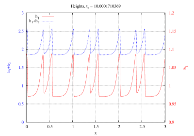
Figure 8: Fluid heights at time $t=10$

We clearly see the formation of roll-waves both at the free surface and at the interface and that they are in phase. We have computed the spatial Fourier transform of this signal: it is composed of $60$ different modes and the first $20$ modes are the most relevant. We also plotted in picture 9 the time evolution of the first two Fourier modes : for $t\in[0,\,1.2]$, the amplitudes of both interface does not vary much and for $t\in[1.2,\,2]$, there is creation of roll-waves which then stabilize.

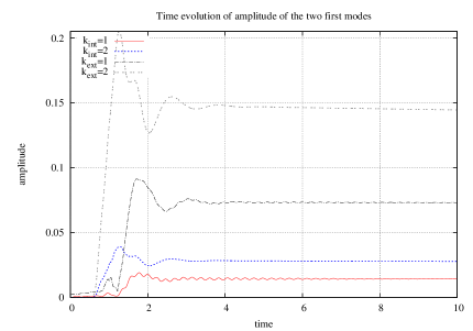
Figure 9: Time evolution of the first two Fourier modes

4 Conclusion

In this paper, we have obtained consistent shallow water equations for bi-layer flows from the Navier Stokes equations in the presence of capillarity. As a byproduct, we carry out a complete spectral stability analysis of bi-layer flows in the low frequency regime. We proved that this system is a generalization of the system of Kuramoto Sivashinsky equations derived in [11] and that it is useful to describe nonlinear waves of arbitrary amplitude in bi layer flows. Numerical simulations then confirm the existence of well known hydrodynamic instabilities, so called roll-waves, which could be localized on the fluid interface or on both interfaces.

This system of shallow water equations is a hyperbolic system in a non conservative form, a common property in shallow water systems describing bi-layer flows. Therefore, there is non uniqueness in the definition of shocks. One possibility would be to derive higher order shallow water models with a vanishing viscosity: the physical viscous term would then select the “physical” jump conditions. For applications purposes, it would be also of interest to derive bi-layer models for non Newtonian fluids in the spirit of [3], where consistant shallow water equations for single thin layers of Bingham and power law fluids.

References

- [1] D.J. Benney, Long waves on liquid films, J. Math.Phys. (N.Y.) 45 (1966) p. 50-155.
- [2] M. Boutounet, L. Chupin , P. Noble , J.-P. Vila, Shallow water equations for Newtonian fluids over arbitrary topographies, Comm. Math. Sci 6 (2008) no. 1, p. 29-55.
- [3] E.D. Fernandez-Nieto, P. Noble, J.-P. Vila, Shallow water equations for Non Newtonian fluids, J. Non-Newtonian Fluid. Mech. 165 (2010) no 13-14, p. 712-732.
- [4] D. Bresch , P. Noble, Mathematical justification of a shallow water model, Methods ans Applications in Analysis 14 (2007) no. 2, p. 87-118.
- [5] G. Dal Maso, P.G. LeFloch, F. Murat, Definition and weak stability of nonconservative products, J. Math. Pure Appl. 74 (1995) p. 483-548.
- [6] R.F. Dressler, Mathematical Solution of the problem of roll-waves in inclined open channels, Comm. Pure. Appl. Math. 2 (1949) p. 149-194.
- [7] J.-F. Gerbeau, B. Perthame, Derivation of viscous Saint-Venant system for laminar shallow water; numerical validation, Discrete Contin. Dyn. Syst. Ser. B 1 (2001), no. 1, p. 89-102.
- [8] T.W. Kao, Stability of two-layer viscous stratified flow down an inclined plane., Phys. Fluids 8 (1965) 812-820.
- [9] T.W. Kao, Role of the interface in the stability of stratified flow down an inclined plane, Phys. Fluids (1965) 2190-2194.
- [10] J.B. Keller, Shallow water theory for arbitrary slopes of the bottom J. Fluid Mech. 489 (2003) p. 345-348.
- [11] I.L. Kliakhandler, Long interfacial waves in multilayer thin films and coupled Kuramoto-Sivashinsky equations, J. Fluid. Mech. 391 (1999) p. 45-65.
- [12] C. Kobayashi, Stability analysis of film flow on an inclined plane II. Multi layer flow, Indust. Coating Res. 2 (1995) p. 65-88.
- [13] A. Harten, P. D. Lax, B. V. Leer On Upstream Differencing and Godunov-Type Schemes for Hyperbolic Conservation Laws, SIAM Review (1983) no. 25, 35-61.
- [14] P. Noble, Roll-waves in general hyperbolic systems with source terms, SIAM J. Appl. Math. 67 (2007), no. 4, p. 1202-1212.
- [15] A. Pumir, P. Manneville, Y. Pomeau, On solitary waves running down on inclined plane J. Fluid Mech 135 (1983), p. 27-50.
- [16] C.Ruyer-Quil, P. Manneville, Modeling film flows down inclined plane Eur. Phys. J. B 6 (1998), p. 277-298.
- [17] C. Ruyer-Quil, P. Manneville, Improved modeling of flows down inclined plane Eur. Phys. J. B 15 (2000), p. 357-369.
- [18] V.Y Shkadov, Wave conditions in the flow of a thin layer of a viscous liquid under the action of gravity Izv. Ak. Nauk SSSR, Mekh. Zhi. Gaza 2 (1967), p.43-51.
- [19] J.-P. Vila, A two moments closure of shallow water type for gravity driven flows, in preparation.
- [20] J.-P. Vila, An Analysis of a Class of Second-Order Accurate Godunov-Type Schemes, SIAM Journal on Numerical Analysis 26,4 (1989), p. 830-853.