Rubidium Rydberg macrodimers

Abstract

We explore long-range interactions between two atoms excited into high principal quantum number $n$ Rydberg states, and present calculated potential energy curves for various symmetries of doubly excited $ns$ and $np$ rubidium atoms. We show that the potential curves for these symmetries exhibit deep ($\sim$ GHz) potential wells, which can support very extended ($\sim$ $\mu$m) bound vibrational states (macrodimers). We present $n$-scaling relations for both the depth $D_{e}$ of the wells and the equilibrium separations $R_{e}$ of these macrodimers, and explore their response to small electric fields and stability with respect to predissociation. Finally, we present a scheme to form and study these macrodimers via photoassociation, and show how one can probe the various $\ell$-character of the potential wells.

1 Introduction

Rydberg atoms have long been studied because of their peculiar properties such as long lifetimes, large cross sections, and very large polarizabilities [1]. These exaggerated properties lead to strong interactions between the Rydberg atoms, which have been experimentally detected in recent years [2, 3]. Such strong Rydberg-Rydberg interactions have fueled a growing interest in the field of quantum computing, and over the past decade, their application for quantum information processing, such as fast quantum gates [4, 5], or quantum random walks [6] have been proposed. Also of particular interest is the excitation blockade effect [7], where one Rydberg atom actually prevents the excitation of other nearby atoms in an ultracold sample [8, 9, 10, 11, 12]. This phenomenon was recently observed in microtraps [13, 14] and a C-NOT gate was implemented using the behavior [15].

Another active area of research with Rydberg atoms is the predicted existence of long-range “exotic molecules”. In one scenario, one atom remains in its ground state, while another atom is excited to a Rydberg state. The most famous examples of this type of interaction are the trilobite and butterfly states, so-called because of the resemblence of their respective wave functions to these creatures. The theoretical framework for such interactions was first proposed in [16], but were not observed until more recently in [17]. The second type of long-range interaction is predicted to occur when both atoms are excited to Rydberg atoms. In [18], it was first predicted that weakly bound macrodimers could be formed from the induced Van der Waals interactions of two such excited atoms. However, more recent work [19] has shown that larger, more stable macrodimers can be formed from the strong mixing between $\ell$-characters of various Rydberg states. Recent measurements have shown signatures of such macrodimers in spectra of cesium Rydberg samples [20].

In this article, we present long-range potential energy curves corresponding to the interaction between pairs of rubidium atoms excited to $ns$ and $np$ Rydberg states. In general, Rydberg-Rydberg interactions will only mix states that share the same molecular symmetry [21, 22]. Thus, only common symmetries between the excited Rydberg molecular state and the state to which it is most strongly coupled are relevant. For rubidium, the doubly excited $ns$ atom pair is most strongly coupled to the $np+(n-1)p$ asymptote, while the doubly excited $np$ atom pair is most strongly coupled to the $ns+(n+1)s$ asymptote. Since all $ss^{\prime}$ states have $m_{j}=\pm\frac{1}{2}$, the only common symmetries with any $pp^{\prime}$ state are $\Omega\equiv|m_{j_{1}}+m_{j_{2}}|=0$, 1. In this manner, we find that the relevant symmetries for the doubly excited $ns$ and $np$ asymptotes are $0_{g}^{+}$, $0_{u}^{-}$ and $1_{u}$. We analyze all three cases for both pairs and show that potential wells exist for all of them. We also describe in detail properties of the bound levels within each well.

The paper is arranged as follows: in §2, we review how to build the basis states used to compute the potential energy curves at long-range, and describe the existence of potential wells for certain asymptotes. In §3, we investigate the effects of small external electric fields on the potential curves, and in §4, we discuss the scaling of the wells with principal quantum number $n$. Finally, in §5, we calculate bound levels supported in those wells, and estimate their lifetimes. We also outline how photoassociation could be used to form and probe macrodimers. This is followed by concluding remarks in §6.

2 Molecular Curves

2.1 Basis States

In this section, we review the general theory for calculating the interaction potential curves. These curves are calculated by diagonalizing the interaction Hamiltonian in the Hund’s case (c) basis set, which is appropriate when the spin-orbit coupling becomes significant and fine structure cannot be ignored, as is the case here.

We first consider two free Rydberg atoms in states $|a\rangle\equiv|n,\ell,j,m_{j}\rangle$ and $|a^{\prime}\rangle\equiv|n^{\prime},\ell^{\prime},j^{\prime},m^{\prime}_{j}\rangle$, where $n$ is the principal quantum number, $\ell$ the orbital angular momentum, and $m_{j}$ is the projection of the total angular momentum $\vec{j}=\vec{\ell}+\vec{s}$ onto a quantization axis (chosen in the $z$-direction for convenience). The long-range Hund’s case (c)  basis states are constructed as follows:

$$|a;a^{\prime};\Omega_{g/u}\rangle\sim|a\rangle_{1}|a^{\prime}\rangle_{2}-p(-1)^{\ell+\ell^{\prime}}|a^{\prime}\rangle_{1}|a\rangle_{2},$$ (1)

where $\Omega=m_{j}+m^{\prime}_{j}$ is the projection of the total angular momentum on the molecular axis and is conserved. The quantum number $p$ describes the symmetry property under inversion and is 1($-$1) for $g(u)$ states.

For $\Omega=0$, we need to additionally account for the reflection through a plane containing the internuclear axis. Such a reflection will either leave the wave function unaffected or it will change the sign of the wave function. We distinguish between these symmetric and antisymmetric states under the reflection operator $\hat{\sigma}_{\nu}$ as follows:

$$|0^{\pm}_{g/u}\rangle=\frac{1\pm\hat{\sigma}_{\nu}}{\sqrt{2}}|0_{g/u}\rangle\,,$$ (2)

where $\hat{\sigma}_{\nu}$ behaves according to the following rules [23, 24]:

$$\hat{\sigma}_{\nu}|\Lambda\rangle =(-1)^{\Lambda}|-\Lambda\rangle$$ (3)

$$\hat{\sigma}_{\nu}|S,M_{S}\rangle =(-1)^{S-M_{S}}|S,-M_{S}\rangle\,.$$ (4)

References [22] and [25] give the technical details for determining which states comprise the basis of the $np+np$ rubidium asymptote. Although the procedure to find the basis states for different molecular asymptotes, such as $ns+ns$, $np+np$, or $nd+nd$, is the same, the states making up these basis sets, in general, will be different. We do not review the procedure for building the basis sets here, but we note that all relevant (i.e. strongly coupled) molecular asymptotes within the vicinity of the asymptotic doubly-excited Rydberg state being considered are included in each respective basis set. We again note here that because doubly excited $ns$ ($np$) rubidium atoms are most strongly coupled to $pp^{\prime}$ ($ss^{\prime}$) states and because only common symmetries of such Rydberg states are allowed to mix, the relevant symmetries for the $ns+ns$ and $np+np$ asymptotic Rydberg states that we consider are $0_{g}^{+}$, $0_{u}^{-}$ and $1_{u}$. As an example, Table 1 lists the basis set for the $0_{g}^{+}$ symmetry near the Rb $70p+70p$ molecular asymptote.

Table 1: Asymptotic $0_{g}^{+}$ molecular states included in the Rb $70p+70p$ basis set, which diagonalize the interaction Hamiltonian (see text). The basis states have been symmetrized with respect to the reflection operator (2) and each $|a_{1};a_{2};0_{g}\rangle$ state is defined by equation (1).

$\frac{1}{\sqrt{2}}\left\{|70s\frac{1}{2},\frac{1}{2};71s\frac{1}{2},-\frac{1}{2};0_{g}\rangle-|70s\frac{1}{2},-\frac{1}{2};71s\frac{1}{2},\frac{1}{2};0_{g}\rangle\right\}$	$\frac{1}{\sqrt{2}}\left\{|68d\frac{3}{2},\frac{1}{2};71s\frac{1}{2},-\frac{1}{2};0_{g}\rangle+|68d\frac{3}{2},-\frac{1}{2};71s\frac{1}{2},\frac{1}{2};0_{g}\rangle\right\}$
$|70p\frac{3}{2},\frac{3}{2};70p\frac{3}{2},-\frac{3}{2};0_{g}\rangle$	$\frac{1}{\sqrt{2}}\left\{|68d\frac{5}{2},\frac{1}{2};71s\frac{1}{2},-\frac{1}{2};0_{g}\rangle-|68d\frac{5}{2},-\frac{1}{2};71s\frac{1}{2},\frac{1}{2};0_{g}\rangle\right\}$
$|70p\frac{3}{2},\frac{1}{2};70p\frac{3}{2},-\frac{1}{2};0_{g}\rangle$	$\frac{1}{\sqrt{2}}\left\{|67d\frac{3}{2},\frac{1}{2};72s\frac{1}{2},-\frac{1}{2};0_{g}\rangle+|67d\frac{3}{2},-\frac{1}{2};72s\frac{1}{2},\frac{1}{2};0_{g}\rangle\right\}$
$\frac{1}{\sqrt{2}}\left\{|70p\frac{3}{2},\frac{1}{2};70p\frac{1}{2},-\frac{1}{2};0_{g}\rangle+|70p\frac{3}{2},-\frac{1}{2};70p\frac{1}{2},\frac{1}{2};0_{g}\rangle\right\}$	$\frac{1}{\sqrt{2}}\left\{|67d\frac{5}{2},\frac{1}{2};72s\frac{1}{2},-\frac{1}{2};0_{g}\rangle-|67d\frac{5}{2},-\frac{1}{2};72s\frac{1}{2},\frac{1}{2};0_{g}\rangle\right\}$
$|70p\frac{1}{2},\frac{1}{2};70p\frac{1}{2},-\frac{1}{2};0_{g}\rangle$	$\frac{1}{\sqrt{2}}\left\{|70d\frac{3}{2},\frac{1}{2};69s\frac{1}{2},-\frac{1}{2};0_{g}\rangle+|70d\frac{3}{2},-\frac{1}{2};69s\frac{1}{2},\frac{1}{2};0_{g}\rangle\right\}$
$\frac{1}{\sqrt{2}}\left\{|69p\frac{3}{2},\frac{3}{2};71p\frac{3}{2},-\frac{3}{2};0_{g}\rangle-|69p\frac{3}{2},-\frac{3}{2};71p\frac{3}{2},\frac{3}{2};0_{g}\rangle\right\}$	$\frac{1}{\sqrt{2}}\left\{|70d\frac{5}{2},\frac{1}{2};69s\frac{1}{2},-\frac{1}{2};0_{g}\rangle-|70d\frac{5}{2},-\frac{1}{2};69s\frac{1}{2},\frac{1}{2};0_{g}\rangle\right\}$
$\frac{1}{\sqrt{2}}\left\{|69p\frac{3}{2},\frac{1}{2};71p\frac{3}{2},-\frac{1}{2};0_{g}\rangle-|69p\frac{3}{2},-\frac{1}{2};71p\frac{3}{2},\frac{1}{2};0_{g}\rangle\right\}$	$\frac{1}{\sqrt{2}}\left\{|68s\frac{1}{2},\frac{1}{2};73s\frac{1}{2},-\frac{1}{2};0_{g}\rangle-|68s\frac{1}{2},-\frac{1}{2};73s\frac{1}{2},\frac{1}{2};0_{g}\rangle\right\}$
$\frac{1}{\sqrt{2}}\left\{|69p\frac{3}{2},\frac{1}{2};71p\frac{1}{2},-\frac{1}{2};0_{g}\rangle+|69p\frac{3}{2},-\frac{1}{2};71p\frac{1}{2},\frac{1}{2};0_{g}\rangle\right\}$	$\frac{1}{\sqrt{2}}\left\{|67f\frac{5}{2},\frac{1}{2};70p\frac{1}{2},-\frac{1}{2};0_{g}\rangle-|67f\frac{5}{2},-\frac{1}{2};70p\frac{1}{2},\frac{1}{2};0_{g}\rangle\right\}$
$\frac{1}{\sqrt{2}}\left\{|69p\frac{1}{2},\frac{1}{2};71p\frac{3}{2},-\frac{1}{2};0_{g}\rangle+|69p\frac{1}{2},-\frac{1}{2};71p\frac{3}{2},\frac{1}{2};0_{g}\rangle\right\}$	$\frac{1}{\sqrt{2}}\left\{|67f\frac{5}{2},\frac{1}{2};70p\frac{3}{2},-\frac{1}{2};0_{g}\rangle+|67f\frac{5}{2},-\frac{1}{2};70p\frac{3}{2},\frac{1}{2};0_{g}\rangle\right\}$
$\frac{1}{\sqrt{2}}\left\{|69p\frac{1}{2},\frac{1}{2};71p\frac{1}{2},-\frac{1}{2};0_{g}\rangle-|69p\frac{1}{2},-\frac{1}{2};71p\frac{1}{2},\frac{1}{2};0_{g}\rangle\right\}$	$\frac{1}{\sqrt{2}}\left\{|67f\frac{5}{2},\frac{3}{2};70p\frac{3}{2},-\frac{3}{2};0_{g}\rangle+|67f\frac{5}{2},-\frac{3}{2};70p\frac{3}{2},\frac{3}{2};0_{g}\rangle\right\}$
$\frac{1}{\sqrt{2}}\left\{|69s\frac{1}{2},\frac{1}{2};72s\frac{1}{2},-\frac{1}{2};0_{g}\rangle-|69s\frac{1}{2},-\frac{1}{2};72s\frac{1}{2},\frac{1}{2};0_{g}\rangle\right\}$	$\frac{1}{\sqrt{2}}\left\{|67f\frac{7}{2},\frac{1}{2};70p\frac{1}{2},-\frac{1}{2};0_{g}\rangle+|67f\frac{7}{2},-\frac{1}{2};70p\frac{1}{2},\frac{1}{2};0_{g}\rangle\right\}$
$\frac{1}{\sqrt{2}}\left\{|68p\frac{3}{2},\frac{3}{2};72p\frac{3}{2},-\frac{3}{2};0_{g}\rangle-|68p\frac{3}{2},-\frac{3}{2};72p\frac{3}{2},\frac{3}{2};0_{g}\rangle\right\}$	$\frac{1}{\sqrt{2}}\left\{|67f\frac{7}{2},\frac{1}{2};70p\frac{3}{2},-\frac{1}{2};0_{g}\rangle-|67f\frac{7}{2},-\frac{1}{2};70p\frac{3}{2},\frac{1}{2};0_{g}\rangle\right\}$
$\frac{1}{\sqrt{2}}\left\{|68p\frac{3}{2},\frac{1}{2};72p\frac{3}{2},-\frac{1}{2};0_{g}\rangle-|68p\frac{3}{2},-\frac{1}{2};72p\frac{3}{2},\frac{1}{2};0_{g}\rangle\right\}$	$\frac{1}{\sqrt{2}}\left\{|67f\frac{7}{2},\frac{3}{2};70p\frac{3}{2},-\frac{3}{2};0_{g}\rangle-|67f\frac{7}{2},-\frac{3}{2};70p\frac{3}{2},\frac{3}{2};0_{g}\rangle\right\}$
$\frac{1}{\sqrt{2}}\left\{|68p\frac{3}{2},\frac{1}{2};72p\frac{1}{2},-\frac{1}{2};0_{g}\rangle+|68p\frac{3}{2},-\frac{1}{2};72p\frac{1}{2},\frac{1}{2};0_{g}\rangle\right\}$	$\frac{1}{\sqrt{2}}\left\{|68f\frac{5}{2},\frac{1}{2};69p\frac{1}{2},-\frac{1}{2};0_{g}\rangle-|68f\frac{5}{2},-\frac{1}{2};69p\frac{1}{2},\frac{1}{2};0_{g}\rangle\right\}$
$\frac{1}{\sqrt{2}}\left\{|68p\frac{1}{2},\frac{1}{2};72p\frac{3}{2},-\frac{1}{2};0_{g}\rangle+|68p\frac{1}{2},-\frac{1}{2};72p\frac{3}{2},\frac{1}{2};0_{g}\rangle\right\}$	$\frac{1}{\sqrt{2}}\left\{|68f\frac{5}{2},\frac{1}{2};69p\frac{3}{2},-\frac{1}{2};0_{g}\rangle+|68f\frac{5}{2},-\frac{1}{2};69p\frac{3}{2},\frac{1}{2};0_{g}\rangle\right\}$
$\frac{1}{\sqrt{2}}\left\{|68p\frac{1}{2},\frac{1}{2};72p\frac{1}{2},-\frac{1}{2};0_{g}\rangle-|68p\frac{1}{2},-\frac{1}{2};72p\frac{1}{2},\frac{1}{2};0_{g}\rangle\right\}$	$\frac{1}{\sqrt{2}}\left\{|68f\frac{5}{2},\frac{3}{2};69p\frac{3}{2},-\frac{3}{2};0_{g}\rangle+|68f\frac{5}{2},-\frac{3}{2};69p\frac{3}{2},\frac{3}{2};0_{g}\rangle\right\}$
$\frac{1}{\sqrt{2}}\left\{|69d\frac{3}{2},\frac{1}{2};70s\frac{1}{2},-\frac{1}{2};0_{g}\rangle+|69d\frac{3}{2},-\frac{1}{2};70s\frac{1}{2},\frac{1}{2};0_{g}\rangle\right\}$	$\frac{1}{\sqrt{2}}\left\{|68f\frac{7}{2},\frac{1}{2};69p\frac{1}{2},-\frac{1}{2};0_{g}\rangle+|68f\frac{7}{2},-\frac{1}{2};69p\frac{1}{2},\frac{1}{2};0_{g}\rangle\right\}$
$\frac{1}{\sqrt{2}}\left\{|69d\frac{5}{2},\frac{1}{2};70s\frac{1}{2},-\frac{1}{2};0_{g}\rangle-|69d\frac{5}{2},-\frac{1}{2};70s\frac{1}{2},\frac{1}{2};0_{g}\rangle\right\}$	$\frac{1}{\sqrt{2}}\left\{|68f\frac{7}{2},\frac{1}{2};69p\frac{3}{2},-\frac{1}{2};0_{g}\rangle-|68f\frac{7}{2},-\frac{1}{2};69p\frac{3}{2},\frac{1}{2};0_{g}\rangle\right\}$
	$\frac{1}{\sqrt{2}}\left\{|68f\frac{7}{2},\frac{3}{2};69p\frac{3}{2},-\frac{3}{2};0_{g}\rangle-|68f\frac{7}{2},-\frac{3}{2};69p\frac{3}{2},\frac{3}{2};0_{g}\rangle\right\}$

2.2 Long-range Interactions

The interaction matrix we consider consists of both the long-range Rydberg-Rydberg interaction and the atomic fine structure. Here, “long-range” refers to the case where no electron exchange takes place i.e. the electronic clouds about both nuclei do not overlap. This occurs when the distance $R$ between the two nuclei is greater than the LeRoy Radius [26]:

$$R_{LR}=2\left[\langle n_{1}\ell_{1}|r^{2}|n_{1}\ell_{1}\rangle^{1/2}+\langle n_{2}\ell_{2}|r^{2}|n_{2}\ell_{2}\rangle^{1/2}\right]\;.$$ (5)

When the distance between the two atoms is larger than $R_{LR}$, the interaction between them is described by the residual Coulomb potential between two non-overlapping charge distributions [27], which can be truncated to give only the dipole-dipole ($V_{d}$) and quadrupole-quadrupole ($V_{q}$) terms. For two atoms lying along the $z$-axis, the $V_{d}$ and $V_{q}$ terms can be simplified to give [28]:

$$V_{L}(R)=-\frac{(-1)^{\ell}4\pi r_{1}^{L}r_{2}^{L}}{\hat{L}R^{\hat{L}}}\sum_{m}{B_{2\ell}^{L+m}Y_{L}^{m}(\hat{r}_{1})Y_{L}^{-m}(\hat{r}_{2})}.$$ (6)

Here, $L=1(2)$ for dipolar (quadrupolar) interactions, $B_{n}^{k}\equiv\frac{n!}{k!(n-k)!}$ is the binomial coefficient, $\vec{r}_{i}$ is the position of electron $i$ from its center, and $\hat{L}\equiv 2L+1$.

Because the molecular basis states are linear combinations of the atomic states determined through symmetry considerations, each matrix element will actually be a sum of multiple interactions, i.e.

$$\langle a;a^{\prime};\Omega_{g/u}|V_{L}|b;b^{\prime};\Omega_{g/u}\rangle = \langle a;a^{\prime}|V_{L}|b;b^{\prime}\rangle-p_{a}(-1)^{\ell_{a}+\ell^{\prime}_{a}}\langle a^{\prime};a|V_{L}|b;b^{\prime}\rangle$$ (7)

$$-p_{b}(-1)^{\ell_{b}+\ell^{\prime}_{b}}\langle a;a^{\prime}|V_{L}|b^{\prime};b\rangle$$

$$+p_{a}p_{b}(-1)^{\ell_{a}+\ell^{\prime}_{a}+\ell_{b}+\ell^{\prime}_{b}}\langle a^{\prime};a|V_{L}|b^{\prime};b\rangle\;,$$

where $|a;a^{\prime}\rangle\equiv|a\rangle_{1}|a^{\prime}\rangle_{2}$ and so on. An analytical expression for the long-range interactions is obtained using angular momentum algebra in terms of $3$-$j$ and $6$-$j$ symbols:

$$\langle 1;2|V_{L}(R)|3;4\rangle=(-1)^{L-1-\Omega+j_{\rm tot}}\sqrt{\hat{\ell_{1}}\hat{\ell_{2}}\hat{\ell_{3}}\hat{\ell_{4}}\hat{j_{1}}\hat{j_{2}}\hat{j_{3}}\hat{j_{4}}}\,\,\,\,\frac{\mathcal{R}_{13}^{L}\mathcal{R}_{24}^{L}}{R^{2L+1}}$$

$$\times\left(\begin{array}[]{ccc}\ell_{1}&L&\ell_{3}\\ 0&0&0\\ \end{array}\right)\left(\begin{array}[]{ccc}\ell_{2}&L&\ell_{4}\\ 0&0&0\\ \end{array}\right)\left\{\begin{array}[]{ccc}j_{1}&L&j_{3}\\ \ell_{3}&\frac{1}{2}&\ell_{1}\\ \end{array}\right\}\left\{\begin{array}[]{ccc}j_{2}&L&j_{4}\\ \ell_{4}&\frac{1}{2}&\ell_{2}\\ \end{array}\right\}$$ (16)

$$\times\sum_{m=-L}^{L}B_{2L}^{L+m}\left(\begin{array}[]{ccc}j_{1}&L&j_{3}\\ -m_{j_{1}}&m&m_{j_{3}}\\ \end{array}\right)\left(\begin{array}[]{ccc}j_{2}&L&j_{4}\\ -\Omega+m_{j_{1}}&-m&\Omega-m_{j_{3}}\\ \end{array}\right)\,,$$ (21)

where $j_{\rm tot}\equiv\sum_{i=1}^{4}{j_{i}}$, $\hat{\ell_{i}}=2\ell_{i}+1,\hat{j_{i}}=2j_{i}+1$, and $\mathcal{R}_{ij}^{L}=\langle i|r^{L}|j\rangle$ is the radial matrix element. For $|1;2\rangle=|3;4\rangle$, the matrix element is given by (2.2) plus the sum of the two atomic asymptotic Rydberg energy values. That is:

$$\langle 1;2|V_{L}(R)|1;2\rangle=\mbox{(\ref{eq:MtxEl})}+E_{1}+E_{2}\,,$$ (22)

with $E_{i}$ given by $-\,\displaystyle\frac{1}{2(n_{i}-\delta_{\ell})^{2}}\,\,,$ where $n_{i}$ is the principal quantum number and $\delta_{\ell}$ is the quantum defect (values given in [29] and [30]). Since $\Delta\ell=0$ dipole transitions are forbidden, only the $L=2$ term of equation (2.2) will contribute in (22).

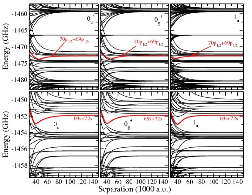
Figure 1: (Color online) Long-range interaction curves for the $0_{u}^{-}$ (left), $0_{g}^{+}$ (middle), and $1_{u}$ (right) symmetries of doubly-excited $ns$ (top row), and $np$ (bottom row) Rb Rydberg atoms near $n=70$. We highlight the potential wells and label their corresponding asymptotic state. Note: All energies are measured from the Rb ionization threshold.

Figure 1 shows the results of diagonalization for the $0_{g}^{+}$, $0_{u}^{-}$ and $1_{u}$ symmetries of the $70s+70s$, and $70p+70p$ asymptotes with no background electric field. In all of these plots, the energies are measured from the ionization threshold of rubidium. We see that all three symmetries feature large potential wells and for the remainder of this paper, we focus our attention on formation properties of bound states within these wells and analyze the stability of these macrodimers. We note here that we also explored the potential curves near the $nd+nd$ asymptotes, but no wells were found; hence we do not display those curves here.

3 Electric Field Dependence

Production and/or detection of macrodimers will rely on external electric fields. In addition, since experiments cannot completely shield the atoms from undesired stray fields, it is important to study their effect on our calculated curves.

Strictly speaking, applying an external electric field $\vec{F}$ breaks the $D_{\infty h}$ symmetry of homonuclear dimers, and consequently, the basis states defined by (1) would no longer be valid. In principle, one then needs to diagonalize the interaction matrix in a basis set containing every possible Stark state, as was done in [31]. However, since the effects of such an electric field should be adiabatic, we assume that the $D_{\infty h}$ symmetry is still approximately valid for small electric fields.

We consider the effects of such an electric field as a perturbation to the original Hamiltonian. In general, an applied electric field will define a quantization axis; the molecular axes of our macrodimers will then be at some random angle to this quantization axis. In that case, one needs to transform the molecular-fixed frame back into the laboratory-fixed frame [32]. To simplify our calculations, we assume that the two Rydberg atoms are first confined in an optical lattice, such that the quantization axes of the macrodimer and the electric field coincide (see figure 2). Such one-dimensional optical lattices have already been used to experimentally excite Rydberg atoms from small Bose-Einstein condensates located at individual sites [33]. We envision a similar one-dimensional optical lattice with the distance between adjacent (or subsequent) sites adjusted to coincide with $R_{e}$, but containing a single atom per site. The lattice could be switched off during the Rydberg excitation to allow a cleaner signal.

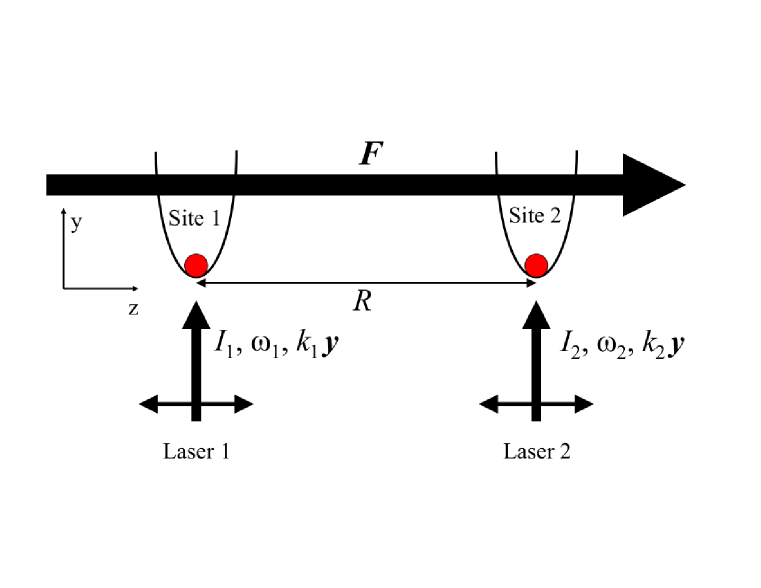
Figure 2: (Color online) Two Rydberg atoms confined within harmonic traps provided by optical lattice sites. The electric field $\mathbf{F}$ is directed along the $z$-axis, coinciding with the molecular axis of the dimer. We also indicate in this cartoon that the two excitation lasers (see section 5.2) propagate in the $y$-direction, but the polarization directions of both lasers are along the $z$-axis.

For an electric field directed along the $z$-axis, the perturbation Hamiltonian for a single atom is given by $Fr\cos{\theta}$, where $F$ is the magnitude of the electric field, $r$ is the distance of the valence electron from its nucleus, and $\theta$ is the angle between $F$ and $r$. We express the new eigenstates (Stark or dressed states) of the perturbed Hamiltonian as a series expansion using the unperturbed asymptotic eigenstates, i.e.

$$|\tilde{a}\rangle_{k}=\sum_{i}b_{k,i}(F)|a_{i}\rangle_{k}\,\,,$$ (23)

where $|a_{i}\rangle_{k}\equiv|n_{i},\ell_{i},j_{i},m_{j}^{(i)}\rangle_{k}$ are the unperturbed (undressed) atomic states of atom $k$, and $b_{k,i}(F)$ are field-dependent eigenvectors, resulting from diagonalization [34]. Here, the index $i$ stands for $n_{i}$, $\ell_{i}$, and $j_{i}$. In Fig. 3, we show the Stark map for $|m_{\ell}|=0$ near $n=69$. Although the limits of this summation are technically $n_{i}\rightarrow n_{max}$ (where $n_{max}$ is the highest $n$ value in the basis) and $\ell_{i}\rightarrow(n_{i}-1)$, we restrict the summation to $(n-2)<n_{i}<(n+2)$ and $\ell_{i}\leq 3$; the $b_{i}(F)$ coefficients are insignificant ($\geq$ 2 orders of magnitude smaller) for states lying outside these bounds. Using the dressed states (23) in (1), we define the dressed molecular states as:

$$|\tilde{a}\rangle_{1}|\tilde{a}\rangle_{2}=\sum_{ij}b_{1,i}(F)b_{2,j}(F)|a_{i}\rangle_{1}|a_{j}\rangle_{2}\,\,.$$ (24)

We then use this basis to redefine the properly symmetrized dressed molecular basis given in Table 1 and to diagonalize the Rydberg-Rydberg interaction matrix.

In Fig. 4, we illustrate the effect of $\vec{F}$ on the curves near $70p+70p$ of the $0_{g}^{+}$ symmetry, in a side-by-side comparison of the curves for $F=0$ and 0.3 V/cm. The atomic Stark states were computed using the method described in [34, 18] and the interaction curves for the “pseudo-symmetry” were obtained by diagonalization of the Rydberg-Rydberg interaction matrix in the dressed molecular basis set (24). We find some minor differences: the Stark effect is most notable in the shifting of the potential curves, especially the asymptotic energies. However, the relative shape of the curves are only slighty changed and most importantly, the large potential well is robust against small electric fields.

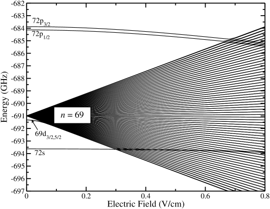
Figure 3: Atomic Rydberg energies vs. the electric field for Rb with $|m_{\ell}|=0$ near $n=69$: the curves labeled by $n=69$ include states with $\ell\geq 3$.

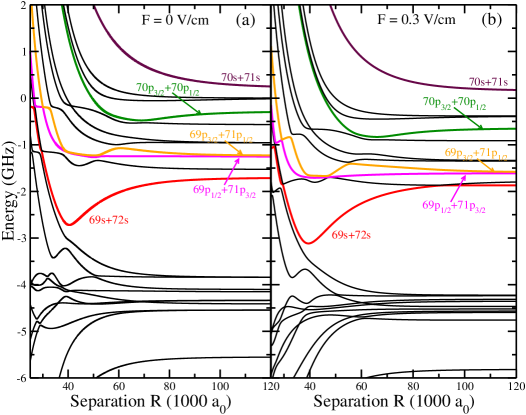
Figure 4: (Color online) $0_{g}^{+}$ molecular curves for Rb $70p+70p$: (a) $F=0$, and (b) $0.3$ V/cm. The states involved in the well correlated to $69s+72s$ are identified (see section 5). The zero-energy is set at the $70p_{3/2}+70p_{3/2}$ asymptote in both plots.

4 Scaling

We focus our attention on the wells correlated to the $(n-1)s+(n+2)s$ asymptote near $np_{3/2}+np_{3/2}$, and those correlated to $(n-1)p_{1/2}+np_{1/2}$ near $ns+ns$, for $F=0$. We calculated the curves for a large range of $n$, and found that the wells follow simple $n$-scaling behaviors (see Fig. 5). As will be discussed in §5, the wells are produced by the mixing of several states with different $\ell$-character. The exact mixing takes place mainly via dipole and quadrupole interactions, and occurs between nearby $n$-states: hence the wells depend on the combination of multipole interaction between states, and the proximity (in energy) of those states.

To derive a simple $n$-scaling behavior for both the depth $D_{e}$ and equilibrium separation $R_{e}$, we assume that the dipole-dipole coupling is the dominant interaction between states, and that the wells are formed as a result of an avoided crossing between two potential curves (see Fig. 5(a)). As mentioned above, the real situation is much more complex, but these assumptions allow for a simple treatment.

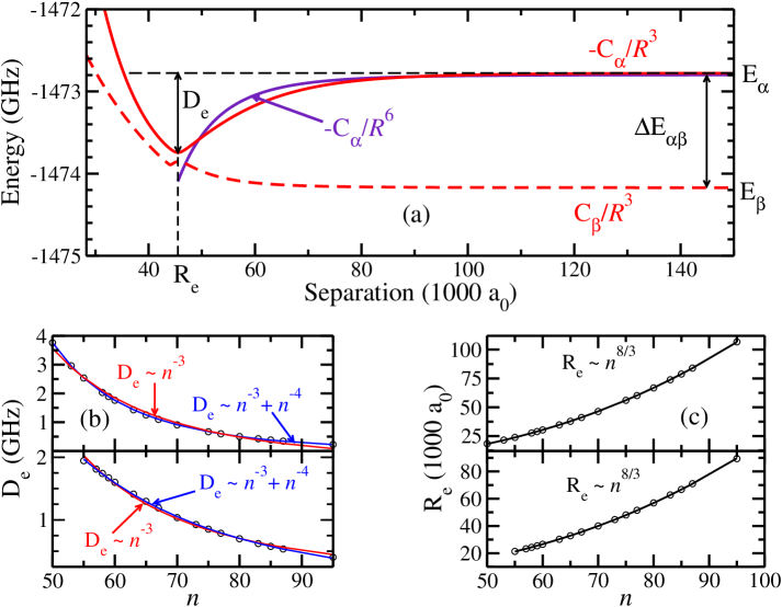
Figure 5: (Color online) (a) Isolated avoided crossing in the $0_{u}^{-}$ symmetry curves of doubly excited $ns$ atoms, which results in the potential well correlated to the $69p_{1/2}+70p_{1/2}$ asymptote. We assume the interactions at the crossing are mostly dipolar in nature (see text) and label the well depth $D_{e}$ and the equilibrium separation $R_{e}$ at the avoided crossing. We also demonstrate that at long range the curves behave as $\sim 1/R^{6}$, but in the $R$-range of the avoided crossing, they behave as $\sim 1/R^{3}$. (b) Scaling relations for the well depth $D_{e}$ vs $n$ for the $0_{u}^{-}$ symmetry of $ns+ns$ (top) and $np+np$ (bottom). (c) Scaling relations for the equilibrium separation $R_{e}$ vs $n$ for the same curves as in (b).

The energy difference $\Delta E_{\alpha\beta}=E_{\alpha}-E_{\beta}$ is defined by the difference between the asymptotes of the two crossing states, $\alpha$ and $\beta$. Here, $\alpha=n_{\alpha_{1}}s+n_{\alpha_{2}}s$, with energy $2E_{\alpha}=-(\nu_{\alpha_{1}}^{-2}+\nu_{\alpha_{2}}^{-2})$ and $\beta=n_{\beta_{1}}p+n_{\beta_{2}}p$, with energy $2E_{\beta}=-(\nu_{\beta_{1}}^{-2}+\nu_{\beta_{2}}^{-2})$. In both energy terms, $\nu_{\gamma_{i}}\equiv n_{\gamma_{i}}-\delta_{\gamma_{i}}$ includes the principal quantum number $n$ and quantum defect $\delta$ of the appropriate atomic state $\gamma_{i}$ of atom $i$. Assuming that the relevant atomic states in a given asymptote are separated by $\Delta n$ of the order unity, we can expand the energies as

$$2E_{\alpha}=-2\frac{\Delta n_{\alpha}}{\nu_{\alpha_{1}}^{3}}\makebox[36.135pt]{ and }2E_{\beta}=-2\frac{\Delta n_{\beta}}{\nu_{\beta_{1}}^{3}}\;,$$ (25)

so that

$$\Delta E_{\alpha\beta} \simeq -\left[\frac{\Delta n_{\alpha}}{\nu_{\alpha_{1}}^{3}}+\frac{\Delta n_{\beta}}{\nu_{\beta_{1}}^{3}}\right]\simeq-\frac{\Delta n_{\alpha}}{\nu_{\alpha_{1}}^{3}}\left[1-\frac{\Delta n_{\beta}}{\Delta n_{\alpha}}\left(1-3\frac{\Delta\nu}{\nu_{\alpha_{1}}}\right)\right]\;,$$ (26)

$$\equiv -A\nu_{\alpha_{1}}^{-3}-B\nu_{\alpha_{1}}^{-4}\;,$$

where we assume $\nu_{\beta_{1}}\simeq\nu_{\alpha_{1}}+\Delta\nu$ with $\Delta\nu$ of order one, and $A=(\Delta n_{\alpha}-\Delta n_{\beta})$ and $B=3\Delta\nu\Delta n_{\beta}$. In the cases leading to our wells, $\Delta n_{\alpha}\simeq\Delta n_{\beta}$ so that the leading dependence is $\Delta E_{\alpha\beta}\propto n^{-4}$.

¿From the sketch depicted in Fig. 5(a), assuming leading dipole-dipole interactions, the equilibrium separation $R_{e}$ occurs at the “intersection” of two attractive and repulsive curves separated by $\Delta E_{\alpha\beta}$, i.e., $\Delta E_{\alpha\beta}-C_{\alpha}/R_{e}^{3}\simeq+C_{\beta}/R_{e}^{3}$, which lead to $R_{e}\simeq[(C_{\beta}+C_{\alpha}]/\Delta E_{\alpha\beta}]^{1/3}$. Our assumption that the two crossing curves behave as $\sim 1/R^{3}$ is valid in the region of the intersection; at larger values of $R$, however ($R\gtrsim$ 80 000 $a_{0}$), the curves behave more like $\sim 1/R^{6}$ (see figure 5). ¿From the scaling $C_{\beta}+C_{\alpha}\propto n^{4}$ and $\Delta E_{\alpha\beta}\propto n^{-4}$, we obtain $R_{e}\propto n^{8/3}$. As for the dissociation energy $D_{e}$, it is simply given by $\Delta E_{\alpha\beta}-C_{\alpha}/R_{e}^{3}\simeq D_{e}$, which scales as $\Delta E_{\alpha\beta}$, i.e. $D_{e}\propto n^{-4}$. Fig. 5(b) shows a plot of $D_{e}$ vs. $n$ for the $0_{u}^{-}$ symmetry of the $ns+ns$ and $np+np$ asymptotes, indicating that $D_{e}$ indeed scales more like $\sim n^{-3}+n^{-4}$ (blue curve) than purely $n^{-3}$ (red curve). For the same wells, Fig. 5(c) shows that $R_{e}$ follows the predicted $n^{8/3}$ scaling. In the interest of space, we do not show plots for all of the symmetries highlighted in Fig. 1, but we note that we find the same approximate scaling for all other symmetries.

Although the analytical derivations above give good agreements with numerically determined values of $D_{e}$ and $R_{e}$, the slight discrepencies, especially with the $np+np$ plots, reflect the more complex nature of the interactions. For example, quadrupole coupling is present in our calculations (although its effect is generally small). We also point out that in the three $np+np$ cases, the formation of each well is not clearly given by an avoided crossing of two curves, but rather by several interacting curves (see next section). Nonetheless, the good agreement depicted in Fig. 5 indicate that these more complicated interactions act only as small corrections.

5 Forming Macrodimers

5.1 Energy Levels and Lifetimes

The wells identified in Fig. 1 support many bound levels. We list the lowest levels for each well in Table 2, together with the corresponding classical inner and outer turning points. For those wells around the $n\sim 70$ asymptotes, the deepest energy levels are separated by about 1$-$2 MHz, corresponding to oscillation periods of a few $\mu$s, rapid enough to allow for several oscillations during the lifetime of the Rydberg atoms (roughly a few hundred $\mu$s for $n=70$). These energy splittings also allow for detection through spectroscopic means. As illustrated by the values of the turning points in Table 2, the bound levels are very extended, leading to macrodimers of a few $\mu$m in size.

Table 2: Energies of the six deepest bound levels (measured from the bottom of the well) and corresponding classical turning points for the $0_{g}^{+}$, $0_{u}^{-}$ and $1_{u}$ symmetries near doubly excited $ns$ and $np$ Rb Rydberg atoms near $n=70$.

• Asymptote	Symmetry	$v$	Energy (MHz)	$R_{1}$ (a.u.)	$R_{2}$ (a.u.)
  $ns+ns$	$0_{g}^{+}$	0	01.035	46,137	46,538
  		1	03.121	45,985	46,688
  		2	05.353	45,870	46,800
  		3	07.477	45,780	46,888
  		4	09.567	45,702	46,963
  		5	11.645	45,630	47,032
  $ns+ns$	$0_{u}^{-}$	0	01.034	45,072	45,488
  		1	03.161	44,913	45,650
  		2	05.262	44,803	45,761
  		3	07.331	44,716	45,854
  		4	09.368	44,639	45,934
  		5	11.392	44,569	46,008
  $ns+ns$	$1_{u}$	0	0.917	36,181	36,600
  		1	2.699	36,038	36,755
  		2	4.467	35,938	36,868
  		3	6.240	35,859	36,963
  		4	7.987	35,789	37,046
  		5	9.747	35,730	37,121
  $np+np$	$0_{g}^{+}$	0	0.831	40,228	40,679
  		1	2.499	40,068	40,849
  		2	4.166	39,959	40,970
  		3	5.824	39,870	41,068
  		4	7.477	39,795	41,154
  		5	9.125	39,728	41,233
  $np+np$	$0_{u}^{-}$	0	0.800	39,753	40,212
  		1	2.414	39,590	40,381
  		2	4.023	39,479	40,509
  		3	5.631	38,390	40,610
  		4	7.234	39,312	40,699
  		5	8.832	39,244	40,778
  $np+np$	$1_{u}$	0	0.708	36,907	37,361
  		1	2.212	36,752	37,535
  		2	3.721	36,632	37,635
  		3	5.219	36,545	37,780
  		4	6.734	36,467	37,870
  		5	8.238	36,399	37,954

As described in §2, the molecular curves are a direct result of the $\ell$-mixing occuring between the electronic basis states (1): each molecular electronic state $|\chi_{\lambda}(R)\rangle$ (corresponding to the potential curve $U_{\lambda}(R)$) is expanded onto the electronic basis states, the amount of mixing varying with $R$:

$$|\chi_{\lambda}(R)\rangle=\sum_{j}c_{j}^{(\lambda)}(R)|j\rangle\,,$$ (27)

where $c_{j}^{(\lambda)}(R)$ are the eigenvectors after diagonalization for each separation $R$, and $|j\rangle$ the electronic basis states (1).

In [19], we showed that the potential well corresponding to the $69s+72s$ asymptote of the $0_{g}^{+}$ symmetry curves near Rb $np+np$ was composed of five nearby asymptotes. We do not review the detailed treatment here, but highlight the significant asymptotes in Fig. 6(a) (left panel). We note that the composition of this well is due to the strong dipole mixing between the five highlighted states, which lead to the well having not only $ss^{\prime}$ character, but also $pp^{\prime}$ character. In the right panel of Fig. 6(a), we illustrate the same information for the well correlated to the $69p_{1/2}+70p_{1/2}$ asymptote near the $70s+70s$ asymptote of the $0_{g}^{+}$ symmetry. Again, we find that the states contributing the most to the existence of this well correspond to asymptotes above $69p_{1/2}+70p_{1/2}$.

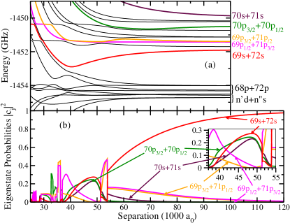
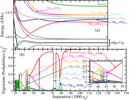
Figure 6: (Color online) (a) $0_{g}^{+}$ symmetry curves of the rubidium $70p+70p$ molecular asymptote (left panel), and the $70s+70s$ molecular asymptote; both plots are zeroed at the ionization level of rubidium. For both panels, we highlight the molecular curves corresponding to the five electronic states contributing the most to the formation of the well (see text). (b) Composition of the 69$s+$72$s$ well (left panel) and of the $69p_{1/2}+70p_{1/2}$ well (right panel): probabilities $|c_{j}(R)|^{2}$ of the electronic states that contribute the most to the formation of the well vs. the nuclear distance $R$. Inset: zoom of the inner region.

In Fig. 6(b), we depict the $\ell$-mixing leading to the potential wells in Fig. 6(a): this is given by the $|c_{j}(R)|^{2}$ coefficients. For both wells near $np+np$ and $ns+ns$, the molecular basis states $|j\rangle$ mixed by the dipole and quadrupole interactions correspond to asymptotes that lie above the asymptote of the wells. In the case of $70p+70p$, the $69s+72s$ molecular level couples strongly to both the $69p+71p$ states (above) and the $68p+72p$ states (below). However, the relative energy differences between the asymptotes results in a much stronger interaction between $69s+72s$ and the $69p+71p$ states than with the $68p+72p$ states. This is why there is little contribution from the $68p+72p$ states in the formation of the well. In the case of $ns+ns$, the states directly below the well correlated to the $69p_{1/2}+71p_{1/2}$ asymptote are $68p+71p$ states. In general, the strength of quadrupole coupling between $np$ states and $n^{\prime}p$ states is very weak. Combining this with the large spacing between the asymptotic energy levels results in minimal contributions from the $68p+71p$ states in the formation of the well.

The insignificant contributions of the states below the potential wells in both cases indicate little chance of predissociation to these lower asymptotes, and hence the macrodimers should be long-lived (limited only by the lifetime of the Rydberg atoms). In [19], we showed that the nonadiabatic coupling between the $69s+72s$ curve and the curves immediately below were very small, leading to metastable macrodimers. For the wells near the $ns+ns$ asymptotes, we reach the same conclusion, i.e. metastable macrodimers with lifetime limited by that of the Rydberg atoms.

5.2 Photoassociation

Exciting two ground state atoms into a bound level via photoassociation (PA) will allow us to probe the different electronic characters mentioned in 5.1. In the following treatment, we describe a PA scheme for the formation of macrodimers bound by the highlighted well of the $0_{g}^{+}$ symmetry of the $np+np$ asymptote (see Fig. 6(a) left panel). We assume that the ground state atoms are first excited to intermediate Rydberg states (treated as the “ground” states) so that the coupling to higher Rydberg states is enhanced. Since the bound states of this particular well have electronic character that is mostly $|ns;n^{\prime}s\rangle$ and $|np;n^{\prime}p\rangle$, we assumed two possible “ground” states making transitions to different $\ell$-character in the well: $40p_{3/2}+40p_{3/2}$ to the $ss^{\prime}$ components, and $41s+41s$ to the $pp^{\prime}$ components. For simplicity, we choose intermediate states near $n\sim 40$ (see inset of figure 7) because the electronic potential curves of these states are asymptotically flat in the $R$ region of the potential well we wish to populate (see [19]); this greatly simplifies the calculations for the PA rates. However, our calculations can of course be modified to fit other experimental parameters and conditions.

Figure 7 shows a schematic for our proposed two-photon formation mechanism for the case of doubly-excited $np$ atoms. The macrodimers we predict could be realized and identified spectroscopically by red-detuning the excitation lasers from the resonant frequency of the $70p_{3/2}+70p_{3/2}$ molecular Rydberg level.

The PA rate ${\sf K}_{v}$ for two atoms into a bound level $v$ can be calculated [35] using

$${\sf K}_{v}\propto I_{1}I_{2}\left|\langle\phi_{v}|\langle\chi_{\lambda}|e^{2}r_{1}r_{2}|\chi_{g}\rangle|\phi_{g}\rangle\right|^{2},$$ (28)

where $I_{1}$ and $I_{2}$ are the intensities of laser 1 and 2, $|\phi_{v}(R)\rangle$ and $|\chi_{\lambda}(R)\rangle$ are the radial and electronic wave functions inside the well, respectively, $|\phi_{g}(R)\rangle$ and $|\chi_{g}(R)\rangle$ are the radial and electronic wave functions of the ground state, respectively, and $r_{i}$ and $e$ are the location and charge of the electron $i$.

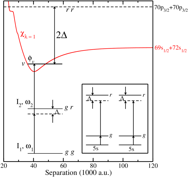
Figure 7: (Color online) Our proposed two-photon photoassociation scheme for the formation of $70p+70p$ rubidium Rydberg macrodimers. The ground state atoms are populated to a bound level inside the well by dual lasers, each of which is red-detuned from the resonance signal of the $70p_{3/2}+70p_{3/2}$ molecular Rydberg state. Inset: Each atom is initially excited to an intermediate Rydberg state, which is considered to be the “ground” state in our discussion (see text). We note that the single atom detuning levels are not to scale.

Using the expression (27) for $|\chi_{\lambda}(R)\rangle$, and assuming that $|\chi_{g}\rangle$ is independent of $R$ (corresponding to a flat curve), we can rewrite (28) as

$${\sf K}_{v}\propto I_{1}I_{2}\sum_{j}\left|(d_{1}d_{2})_{j}\right|^{2}\left|\int_{0}^{\infty}\!\!\!\!dR\phi_{v}^{*}(R)c_{j}^{*}(R)\psi_{g}(R)\right|^{2},$$ (29)

where $d_{1}=\langle n_{j}\ell_{j}|er_{1}|n_{g}\ell_{g}\rangle$ and $d_{2}=\langle n^{\prime}_{j}\ell^{\prime}_{j}|er_{2}|n^{\prime}_{g}\ell^{\prime}_{g}\rangle$ are the electronic dipole moments between electronic states $|a_{g};a^{\prime}_{g}\rangle$ and $|a_{j};a^{\prime}_{j}\rangle$ for atom 1 and atom 2, respectively.

In [19], we presented PA rate calculations for bound levels in the potential well correlated to the $69s+72s$ asymptote from a flat radial ground state distribution. The results of the PA rate against the detuning $\Delta$ from the atomic 70$p_{3/2}$ levels are shown in Fig. 8(a). Since the general expression for the PA rate (29) is proportional to the dipole moments and the laser intensities, our calculated rates are given in arbitrary units set to a maximum of one (for the strongest rate starting from $41s+41s$). In fact, once a pair of atoms has been excited to the “ground” state with fixed laser intensities, the PA rate plotted in Fig. 8 represents the probability of forming a macrodimer; the transition from the 5$s$ Rb atoms to the intermediate “ground” state atoms can easily be saturated so that the PA process always starts with a pair of $40p_{3/2}+40p_{3/2}$ or $41s+41s$. We compare these PA rates to those obtained if the ground state radial wave function $\phi_{g}(R)$ is assumed to be a gaussian centered on $R_{e}$ with a standard deviation of 14 500 $a_{0}$ (roughly half the FWHM of the potential well) in Fig. 8(b). The choice of a gaussian approximates the wave function obtained by thermally averaging harmonic oscillator wave functions over a harmonic trapping potential (e.g. in an optical lattice) for both “ground” state atoms. In those plots, the PA rates starting from both atoms in $40p_{3/2}$ are shown in red and from $41s$ in turquoise, respectively. The rapid oscillation between large rates for an even bound level ($v=0,2,4,\dots$) and small rates for odd levels ($v=1,3,5,\dots$) gives the apparent envelope of the PA signal. This behavior is due to the oscillatory nature of the radial wave functions inside the well $\phi_{v}(R)$: the integral in equation (29) will be near zero for odd wavefunctions. We highlight this for the gaussian $\psi_{g}(R)$ distribution of $40p_{3/2}+40p_{3/2}$ in (c) and $41s+41s$ in (d), where we show a zoom of the deepest levels $v$ (on a log-scale).

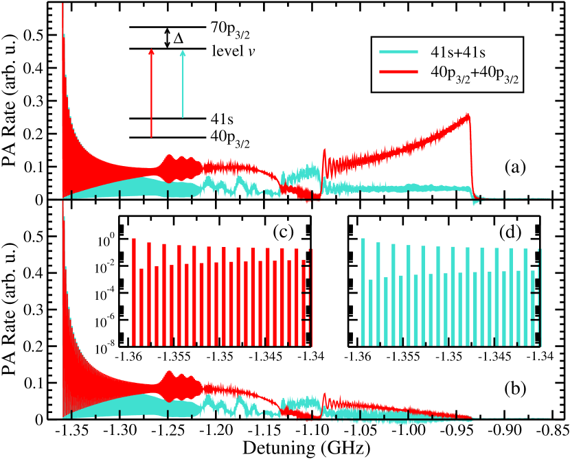
Figure 8: (Color online) PA rate vs. the detuning $\Delta$ from the $70p_{3/2}$ atomic state for (a) a constant radial ground state distribution and (b) a gaussian radial ground state distribution - both on linear scales set to a maximum of 1. The $|41s;41s\rangle$ state populates the $pp^{\prime}$ character in the well (turquoise), and the $|40p_{3/2};40p_{3/2}\rangle$ the $ss^{\prime}$ (red). Plots (c) and (d) show the rates for the deepest levels of the gaussian distribution on a logarithmic scale (see text).

We see in plots (a) and (b) of Fig. 8 that the signature of a macrodimer would manifest itself by the appearance of a signal starting at $\Delta\sim-0.93$ GHz red-detuned from the 70$p_{3/2}$ atomic level, and ending abruptly at $\sim-1.36$ GHz. The shape of the signals indicate that the rates can reveal details of the $\ell$-mixing inside the potential well; for example, both plots show that the $\mathsf{K}_{v}$ mimic the probabilities $|c_{j}(R)|^{2}$ shown in figure 6(b). The progressive decrease of the $41s$ signal beginning at $-$1.36 GHz, followed by sharp increases between $-$1.22 and $-$1.16 GHz correspond to the slow decreases of the $pp^{\prime}$ components between $R\sim$ 40 000 $-$ 50 000 $a_{0}$ and their sharp increases around $R\sim$ 33 000 $-$ 35 000 $a_{0}$. For the $40p_{3/2}$ signal, the major feature common to both (a) and (b) is the significant drop in ${\sf K}_{v}$ between $-1.13$ and $-1.09$ GHz, which mirrors the decrease in the $ss^{\prime}$ states between $R\sim$ 52 000 $-$ 55 000 $a_{0}$ in Fig. 6(b). As noted in [19], this range of frequency with a noticeable drop in the PA rate could serve as a switch to excite or not excite a macrodimer, depending on the “ground” state being used. We also note that in both cases, the signals for the $40p_{3/2}+40p_{3/2}$ “ground” state are higher overall across the $R$ regime of the well, with a few exceptions. This indicates that despite the presence of the $pp^{\prime}$ character, this well is still largely composed of $ss^{\prime}$ character.

As expected, the gaussian ground state distribution shares many qualitative features with the constant ground state distribution. We considered both ground state distributions having populations in the $R$ range of $\sim$ 30 000 to 70 000 $a_{0}$. Normalizing both ground state distributions over this range yielded slightly larger signal rates in the deepest part of the well for the gaussian, corresponding to its peak. However, the major difference between Fig. 8(a) and (b) is noticeable in both the $40p_{3/2}+40p_{3/2}$ and the $41s+41s$ rate signals between $\Delta\sim-1.09$ and $-$0.85 GHz. Whereas the uniform distribution shows a steady $41s+41s$ signal and a steady increase of the $40p_{3/2}+40p_{3/2}$ signal, the gaussian distribution shows both signals rapidly decreasing. As we chose to center the gaussian at the minimum of the well, the decrease in both signals obviously corresponds to the decreasing probability of the gaussian distribution in this $R$ regime (i.e. the tails). If one wanted to take advantage of the large, isolated $69s72s$ character at higher $R$, this could easily be accomplished by recentering the gaussian appropriately.

6 Conclusion

We have presented long-range interaction potential curves for the $0_{g}^{+}$, $0_{u}^{-}$, and $1_{u}$ symmetries of doubly excited $ns$ and $np$ Rydberg atoms and have demonstrated the existence of potential wells between these excited atoms. These wells are very deep and very extended, due to the strong $\ell$-mixing between the various electronic Rydberg states. These wells are robust against small electric fields and support several bound vibrational levels, separated by a few MHz, which could be detected in spectroscopy experiments. The macrodimers corresponding to these bound vibrational levels are stable with respect to predissociation and have lifetimes limited only by the Rydberg atoms themselves. These macrodimers could be realized through population of the vibrational energy levels by photoassociation, resulting in a detectable signal that could be used to probe the various $\ell$-character of the potential well.

In conclusion, we note that the detection of such extended dimers could facilitate studies in a variety of areas. For example, the effect of retardation on the interaction at very large separation, which becomes important if the photon time-of-flight between the atoms is comparable to the classical orbital period of a Rydberg electron around its core [18], could potentially be probed experimentally. Another example relates to chemistry of molecules with high internal energy; a third atom approaching a macrodimer could quench its internal state to lower levels, or could potentially react with the molecule at very large distances and create a new product such as trilobite or butterfly Rydberg molecules [16]. Finally, as mentioned in the introduction, Rydberg atoms are being investigated intensively for quantum information processing, e.g. using the blockade mechanism [7], and the possibility of frequency ranges where the PA rate is strong or weak due to the $\ell$-character mixing could potentially be used as a quantum mechanical switch. These few examples illustrate some possible applications of macrodimers.

References

- [1] Gallagher T 1994 Rydberg Atoms (Cambridge, United Kingdom: Cambridge University Press)
- [2] Anderson W R, Veale J R and Gallagher T F 1998 Phys. Rev. Lett. 80 249–252
- [3] Mourachko I, Comparat D, de Tomasi F, Fioretti A, Nosbaum P, Akulin V M and Pillet P 1998 Phys. Rev. Lett. 80 253–256
- [4] Jaksch D, Cirac J I, Zoller P, Rolston S L, Côté R and Lukin M D 2000 Phys. Rev. Lett. 85 2208–2211
- [5] Protsenko I E, Reymond G, Schlosser N and Grangier P 2002 Phys. Rev. A 65 052301
- [6] Côté R, Russell A, Eyler E and Gould P L 2006 New Journal of Physics 8 1–10
- [7] Lukin M D, Fleischhauer M, Cote R, Duan L M, Jaksch D, Cirac J I and Zoller P 2001 Phys. Rev. Lett. 87 037901
- [8] Tong D, Farooqi S M, Stanojevic J, Krishnan S, Zhang Y P, Côté R, Eyler E E and Gould P L 2004 Phys. Rev. Lett. 93 063001
- [9] Singer K, Reetz-Lamour M, Amthor T, Marcassa L G and Weidemüller M 2004 Phys. Rev. Lett. 93 163001
- [10] Liebisch T C, Reinhard A, Berman P R and Raithel G 2005 Phys. Rev. Lett. 95 253002
- [11] Vogt T, Viteau M, Zhao J, Chotia A, Comparat D and Pillet P 2006 Phys. Rev. Lett. 97 083003
- [12] Heidemann R, Raitzsch U, Bendkowsky V, Butscher B, Löw R and Pfau T 2008 Phys. Rev. Lett. 100 033601
- [13] Gaëtan A, Miroshnychenko Y, Wilk T, Chotia A, Viteau M, Comparat D, Pillet P, Browaeys A and Grangier P Nature Physics 5
- [14] Urban E, Johnson T A, Henage T, Isenhower L, Yavuz D D, Walker T G and Saffman M 2009 Nature Physics 5 110–114
- [15] Isenhower L, Urban E, Zhang X L, Gill A T, Henage T, Johnson T A, Walker T G and Saffman M 2010 Phys. Rev. Lett. 104 010503
- [16] Greene C H, Dickinson A S and Sadeghpour H R 2000 Phys. Rev. Lett. 85 2458–2461
- [17] Bendowsky V, Butscher B, Nipper J, Shaffer J P, Löw R and Pfau T 2009 Nature 458 1005–1008
- [18] Boisseau C, Simbotin I and Côté R 2002 Phys. Rev. Lett. 88 133004
- [19] Samboy N, Stanojevic J and Côté R 2011 Phys. Rev. A 83 050501
- [20] Overstreet K R, Schwettmann A, Tallant J, Booth D and Shaffer J P 2009 Nature Physics 5 581–585
- [21] Marinescu M 1997 Phys. Rev. A 56 4764–4773
- [22] Stanojevic J, Côté R, Tong D, Farooqi S, Eyler E and Gould P 2006 Eur. Phys. J. D 40 3–12
- [23] Bernath P 2005 Spectra of Atoms and Molecules (New York, New York: Oxford University Press)
- [24] Brown J and Carrington A 2003 Rotational Spectroscopy of Diatomic Molecules (Cambridge, United Kingdom: Cambridge University Press)
- [25] Stanojevic J, Côté R, Tong D, Eyler E E and Gould P L 2008 Phys. Rev. A 78 052709
- [26] LeRoy R J 1974 Can. J. Phys. 52 246–256
- [27] Dalgarno A and Davison W 1966 The calculation of van der waals interactions (Advances in Atomic and Molecular Physics vol 2) ed Bates D and Estermann I (Academic Press) pp 1 – 32
- [28] Marinescu M and Dalgarno A 1995 Phys. Rev. A 52 311–328
- [29] Li W, Mourachko I, Noel M W and Gallagher T F 2003 Phys. Rev. A 67 052502
- [30] Han J, Jamil Y, Norum D V L, Tanner P J and Gallagher T F 2006 Phys. Rev. A 74 054502
- [31] Schwettmann A, Crawford J, Overstreet K R and Shaffer J P 2006 Phys. Rev. A 74 020701
- [32] Tscherbul T, Suleimanov Y, Aquilanti V and Krems R 2009 New Journal of Physics 11, 055021
- [33] Viteau M, Bason M G, Radogostowicz J, Malossi N, Ciampini D, Morsch O and Arimondo A 2011, arXiv:1103.4232
- [34] Zimmerman M L, Littman M G, Kash M M and Kleppner D 1979 Phys. Rev. A 20 2251–2275
- [35] Côté R and Dalgarno A 1998 Phys. Rev. A 58 498–508