Vacuum Solution of a Linear Red-Shift Based Correction in $f(R)$ Gravity

Abstract

In this paper we have considered a red-shift based linear correction in derivative of action in the context of vacuum $f(R)$ gravity. Here we have found out that the linear correction may describe the late time acceleration which is appeared by SNeIa with no need of dark energy. Also we have calculated the asymptotic action for the desired correction. The value of all solutions may reduce to de’ Sitter universe in the absence of correction term.

1 Introduction

The recent data coming from the luminosity distance of SuperNovae Ia (SNeIa) [1], wide surveys on galaxies [2] and the anisotropy of cosmic microwave background radiation [3] suggest that the Universe is undergoing an accelerating expansion. Large Scale Structure formation [4], Baryon Oscillations [5] and Weak Lensing [6] also suggest such an accelerated expansion of the Universe. Actually, identifying the cause of this late time acceleration is one of the most challenging problems of modern cosmology. Several approaches being responsible for this expansion, have been proposed in the literature. A positive cosmological constant can lead to accelerated expansion of the universe but it is plagued by the fine tuning problem [7]. The cosmological constant may be interpreted either geometrically as modifying the left hand side of Einstein’s equation or as a kinematic term on the right hand side with the equation of state parameter $w=-1$. Another approach can further be generalized by considering a source term with an equation of state parameter $w<-1/3$. Such kinds of source terms have collectively come to be known as Dark Energy. Various scalar field models of dark energy have been considered in literature [8]. All the dark energy based theories assume that the observed acceleration is the outcome of the action of a still unknown ingredient added to the cosmic pie. In terms of the Einstein equations, $G_{\mu\nu}=\chi T_{\mu\nu}$, such models are simply modifying the right hand side including in the stress–energy tensor with something more than the usual matter and radiation components.

On the other hand, as a radically different approach, one can also try to leave unchanged the source side, but rather than modifying the left hand side of Einstein field equations. In a sense, one is therefore interpreting cosmic acceleration as a first signal of the breakdown of the laws of physics as described by the standard General Relativity (GR). Extending GR, not simply given its positive results, opens the way to a large class of alternative theories of gravity ranging from extra dimensions [9] to non-minimally coupled scalar fields [10]. In particular, we will be interested here in fourth order theories [11] based on replacing the scalar curvature $R$ in the Hilbert–Einstein action with a generic analytic function $f(R)$ which should be reconstructed starting from data and physically motivated issues. Also referred to as $f(R)$ gravity, these models have been shown to be able to fit both the cosmological data and Solar System constraints in several physically interesting cases [12]. These theories are also referred to as ’extended theories of gravity’, since they naturally generalize General Relativity. It has been predicted that the universe might have been appeared from an inflationary phase in the past. It is also believed that the present universe is passing through a phase of the cosmic acceleration. Vacuum solutions of $f(R)$ gravity theories are one of interesting subjects which are obtained for constant Ricci scalar [13, 14, 15, 16], while it is possible to derive non constant curvature scalar vacuum solutions.

In this paper we would like to note that $f(R)$ gravity theory is a powerful approach to describe dynamical behavior of the Universe via an unusual approach. Actually we consider vacuum solutions of $f(R)$ gravity. But there is a difference with other vacuum solutions. This way we do not assume constant scalar curvature to obtain vacuum solution. Vacuum solutions of modified $f(R)$ gravity would like to explain the late time phase transition of cosmological parameters like deceleration parameter without the need for dark companion of the Universe, just by pure geometry.

The pioneering works on reconstruction of modified action through inverse method are done by the authors of Ref. [13, 14, 15, 16]. They developed a general scheme for cosmological reconstruction of modified $f(R)$ gravity in terms of e-folding (or red-shift) without using auxiliary scalar in intermediate calculations. Using this method, it is possible to construct the specific modified gravity which contains any requested FRW cosmology. The number of $f(R)$ gravity examples is used where the following background evolutions may be realized: $\Lambda CDM$ epoch, deceleration with subsequent transition to effective phantom superacceleration leading to Big Rip singularity, deceleration with transition to transit phantom phase without future singularity, oscillating universe. It is important that all these cosmologies may be realized only by modified gravity without the use of any dark components. In this essay, we try to reconstruct an appropriate action for the modified gravity through the semi-inverse solution method. We do not assume any FRW cosmology to reconstruct its related $f(R)$ action. Our starting point is some modification in deriving from a generic action which is depended on red-shift.

In section II, we have a briefer review of modified field equations. In section III, we introduce our model and its results in field solutions. In section IV, we study the evolution of deceleration parameter under considered model and its related dark energy Equation of State (EoS). In section V, we calculate an approximated value for correction parameter which is in accordance with SNeIa data from observational constraints. In section VI, we try to reconstruct the original action which may produce our desired corrections and in section VII we examine the local tests for the obtained action. Section VIII is conclusion of this paper.

2 Modified field equations

The action of modified theory of gravity is given by

$$S=\int d^{4}x\sqrt{-g}\bigg{[}\frac{1}{2\kappa}f(R)+L_{m}\bigg{]},$$ (1)

where $L_{m}$ is the matter action such as radiation, baryonic matter, dark matter and so on which we do not consider them in field equation. In this essay, we consider the flat Friedmann Robertson Walker, (FRW) background, so that the gravitational field equations for $f(R)$ modified gravity are provided by the following form

$$-3\frac{\ddot{a}}{a}f^{\prime}+3\frac{\dot{a}}{a}\dot{R}f^{\prime\prime}+\frac{1}{2}f=0,$$ (2)

$$[\frac{\ddot{a}}{a}+2\frac{\dot{a}^{2}}{a^{2}}]f^{\prime}-2\frac{\dot{a}}{a}\dot{R}f^{\prime\prime}-\dot{R}^{2}f^{\prime\prime\prime}-\ddot{R}f^{\prime\prime}-\frac{1}{2}f=0.$$ (3)

where the overdot denotes a derivative with respect to $t$, and the prime denotes a derivative with respect to $R$, $a(t)$ is the scale factor and $H=\dot{a}(t)/a(t)$ is the Hubble parameter. Eliminating $f$ between Eqs. (2) and (3) results:

$$-2[\frac{\ddot{a}}{a}-(\frac{\dot{a}}{a})^{2}]f^{\prime}+\frac{\dot{a}}{a}\dot{R}f^{\prime\prime}-\ddot{R}f^{\prime\prime}-\dot{R}^{2}f^{\prime\prime\prime}=0.$$ (4)

Which can be changed in the form of:

$$2\dot{H}F-H\dot{F}+\ddot{F}=0,$$ (5)

where $F=df/dR$. Eq. (5) is a second order differential equation of $F$ with respect to time, in which both of $F$ and $H$ are undefined. The usual method to solve Eq. (5) is based on definition of $f(R)$.

Changing the variable of the above equation from $t$ to a new variable like the number of e-folding, $N$ was done in [14, 15, 16]. The variable $N$ is related to the redshift, $z$ by $e^{-N}=1+z$. They solve the cosmological dynamic equation by definition of Hubble parameter as a function of $N$ in a general form. Then they rewrite the equation by redefinition of the variable from the number of e-folding to the Ricci scalar and solve it with respect to the Ricci scalar. Thus they could demonstrate that modified $f(R)$ gravity may describe the $\Lambda CDM$ epoch without any need for introducing the effective cosmological constant, non-phantom matter and phantom matter. In this paper we would like to replace the variable of Eq. (5) by red-shift, $z$, directly to solve the dynamical equation for a specific red-shift depended action.

Each redshift, $z$ has an associated cosmic time $t$ (the time when objects are observed with redshift $z$ emitting light), so we can replace all the differentials with respect to $t$ by $z$ via:

$$\frac{d}{dt} = \frac{da}{dt}\frac{dz}{da}\frac{d}{dz},$$ (6)

$$= -(1+z)H(z)\frac{d}{dz},$$

where we use $1+z={a_{0}}/{a}$, and we consider $a_{0}=1$, in the present time. Now, we can replace the variable of Eq. (5) from $t$ to $z$ by using Eq. (6), and we obtain a first order differential equation for $H^{2}$ with respect to $z$ as:

$$\frac{d}{dz}H(z)^{2}=P(z)H(z)^{2},$$ (7)

where $P(z)$ is a function with respect to $z$, which depends on the definition of $F$ with respect to $z$ as:

$$P(z)=\frac{2(1+z)(d^{2}F/dz^{2})+4(dF/dz)}{2F-(1+z)(dF/dz)}.$$ (8)

Now we may solve Hubble parameter that depends on the definition of $F(z)$. This may happen by analytical calculations or numerical approaches which is based on selection of $F(z)$. Since there could be many choices to select the function of $F(z)$, we have decided to add a linear correction term to General Relativistic limit of $F(R)$ value, which is discussed in the following section.

3 Model selection and its solution

Since we do not know the determined function of $F(z)$, would like to consider a linear correction of red-shift as

$$F(z)=F_{0}(1+\alpha z),$$ (9)

in which for $\alpha=0$ we have $F(z)=F_{0}$. In this case Eq. (7) has a solution such as $H(z)^{2}=H_{0}^{2}$ in which $H_{0}$ is a constant. This case will reproduce de’ Sitter solution of vacuum Universe that is expanded with a constant velocity. Since the value of $H_{0}$ is independent of $F_{0}$ we may fix it to $F_{0}=1$ to recover GR or transfer its effect to gravitational constant by normalization. For $\alpha\neq 0$ we have our linear correction. In this case Eq. (7) has a solution such as

$$H(z)^{2}=H_{\alpha}^{2}\big{[}1-\frac{1}{2}\alpha(1-z)\big{]}^{4},$$ (10)

where $H_{\alpha}^{2}=H_{0}^{2}/(1-\alpha/2)^{4}$. It is clear that it may reduce to de’ Sitter case in the absence of $\alpha$.

4 Cosmic dynamics and EoS

Deceleration parameter, $q$ in cosmology is a dimensionless measure of the cosmic acceleration of the expansion of space in a FRW universe. It is defined by:

$$q=-\frac{\ddot{a}a}{\dot{a}^{2}}=-1-\frac{\dot{H}}{H^{2}}.$$ (11)

here we change the variable of Eq. (11) from $t$ to $z$ then we will have evolution of deceleration parameter with respect to redshift as:

$$q(z) = -1+\frac{1+z}{2H(z)^{2}}\frac{dH(z)^{2}}{dz},$$ (12)

$$= -1+\frac{1+z}{2}P(z),$$ (13)

which only depends on $P(z)$ for vacuum solution. Since we would like to study the first order correction of $F(z)$ we put the modified model in Eq. (13) to obtain

$$q(z)=-1+\frac{2\alpha(1+z)}{2-\alpha(1-z)}.$$ (14)

Transition point from deceleration to acceleration phase ($q(z)=0$) obtains as

$$z_{T}=\frac{2-3\alpha}{\alpha},$$ (15)

which is a constraint for our correction parameter as $0<\alpha<2/3$ to have a transition point in recent positive red-shifts, but it should not be close to zero because this value will shoot the transition to high red-shifts. On the other hand as it is shown in Fig. (1) for all the values of $\alpha<2/3$ universe is under acceleration.

Figure 1: $q(z=0)$ with respect to $\alpha$.

Also evolution of deceleration parameter from high red-shifts to the future is shown in Fig. (2). Another result of Eq. (14) is for large red-shifts, $q(z)\rightarrow 1$ which is the value of deceleration parameter in radiation era.

Figure 2: $q(z=0)$ with respect to $\alpha$.

The equivalent form of dark energy Equation of State (EoS) which corresponds to selected $F(z)$ is obtained as

$$\omega(z) = -1+\frac{1+z}{3H(z)^{2}}\frac{dH(z)^{2}}{dz},$$ (16)

$$= -1+\frac{4\alpha(1+z)}{3[2-\alpha(1-z)]},$$ (17)

which is reduced to de’ Sitter EoS that is equal to $\omega=-1$ when $\alpha=0$. Fig. (3) shows the range of the predicted value of EoS with respect to acceptable values of $\alpha$.

Figure 3: $\omega(z=0)$ with respect to $\alpha$.

Also evolution of EoS from high red-shifts to low red-shifts is shown in Fig. (4). On the other hand Eq. (17) shows that for red-shifts that are large enough, $\omega(z)\rightarrow 1/3$ which is EoS in radiation era, while we have solved modified Friedmann equations for vacuum.

Figure 4: Evolution of $\omega(z)$ for $\Lambda CDM$ (solid line) with $\Omega_{m}=0.3$ and $\Omega_{\Lambda}=0.7$, and for our model with correction parameters $\alpha=0.5$ (dotted line), $\alpha=0.4$ (dashed line) and $\alpha=0.3$ (dashed-dotted line).

5 Supernovae constraint

In the following we would like to constraint our model parameters in comparison with observational data sets. Another main late time cosmological constraint which is tested for the above simple example is SNeIa distance module with respect to redshift constraint. In this comparison we used the Union2 data set [20] which provide 557 SNeIa specifications. According to the value of numerical results which was gotten in comparison with SNeIa data set from usual $\chi^{2}$ algorithm, we discover that for $\alpha=0.418$, $h=0.697$ where $h$ is the reduced Hubble parameter and $\chi^{2}=545.329$, so the ratio of chi square error to the number of freedom is about $0.983$. The result of this calculation is shown in Fig. (5).

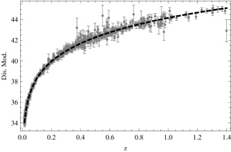
Figure 5: Accordance between Union2 SNeIa data and late time linear correction of our model for $\alpha\approx 0.418$ and $h\approx 0.697$.

6 Reconstruction of $f(R)$ action

Specification of modified action is one of interesting subjects in the story of $f(R)$ gravity. Here we may reconstruct the action via a semi inverse solution approach. The Ricci scalar is defined as

$$R=6(\dot{H}+2H^{2}),$$ (18)

and if we change the variable of this equation from time to red-shift we have

$$R(z)=3[4H(z)^{2}-(1+z)\frac{dH(z)^{2}}{dz}].$$ (19)

The Ricci scalar for the Hubble parameter of Eq. (10) is obtained from Eq. (19) as

$$R(z)=R_{\alpha}\bigg{[}1-\frac{1}{2}\alpha(1-z)\bigg{]}^{3},$$ (20)

where

$$R_{\alpha}=\frac{12(1-\alpha)H_{0}^{2}}{(1-\alpha/2)^{4}},$$ (21)

which will be reduced to another constant in $\alpha=0$ and we may name it the present value of Ricci scalar $R_{0}=12H_{0}^{2}$. Changes of modified Ricci scalar is shown in Fig. (6). If we suppose the value of cosmological constant, $\Lambda=3H_{0}^{2}$ then we have a simplified relation between the present value of curvature scalar and cosmological constant as $R_{0}=4\Lambda$. We may use these equalities to find behavior of the modified solutions in the constraint regions.

Figure 6: Evolution of $R/R_{0}$ with respect to $z$ for three values of correction parameter. The crossing points are not unique.

Figure 7: Change of $f(R)$ with respect to $R$ for three values of correction parameter, $\alpha=0$ in dashed line, $\alpha=0.3$ in dot-dashed line and $\alpha=0.6$ in dotted line. Solid line shows variation of GR action with cosmological constant which is de’ Sitter action.

One of the simple solutions to achieve the desired action is eliminating of $z$ between $F(z)$ and $R(z)$ which leads us to reach the equation

$$F(R)=2(\frac{R}{R_{\alpha}})^{1/3}+\alpha-1.$$ (22)

It is clear that, the derivative of action is different from GR plus cosmological constant or de’ Sitter model. But in the case of $\alpha=0$ or $R_{\alpha}=R_{0}$, we would like to recover de’ Sitter solution. Then by using Eq. (20) we obtain $R=R_{0}$ and then $F(R)=1$ which is equal to the GR or de’Sitter model. Because GR action differs from de’Sitter action only in a constant term.

Now we can calculate $f(R)$ by integrating of Eq. (22) with respect to $R$ as

$$f(R)=R\big{[}\frac{3}{2}(\frac{R}{R_{\alpha}})^{1/3}+\alpha-1\big{]}+C,$$ (23)

where $C$ is constant of integration. Since we would like to recover de’ Sitter model in the absence of correction term, $\alpha$ we must find the true constraint on the constant of integration. we can determine the constraint by comparing the value of de’ Sitter action with the action of Eq. (23) when $\alpha=0$ or $R=R_{0}$. The standard form of de’ Sitter action is $f_{d}(R)=R-2\Lambda$. Since the scalar curvature of de’ Sitter universe is a constant, then we can determine the value of $f_{d}(R)$ in the presence of constant curvature. If we solve the standard algebraic equation of $f(R)$ gravity as $2f_{d}(R)-RF_{d}(R)=0$ we can find $R_{0}=4\Lambda$. Then the value of de’ Sitter action in the case of $R=R_{0}$ is $f_{d}(R_{0}=4\Lambda)=2\Lambda$ which is equal to $R_{0}/2$.

For the case of our obtained action from Eq. (23), we have $f(R=R_{0})=R_{0}/2+C$ when $\alpha=0$. Since we would like to have the same solution for de’ Sitter model and our obtained action in present of $R=R_{0}$ we force constant of integration, $C$ to be equal to zero.

Therefore the obtained action in its constrained form would be

$$f(R)=R\big{[}\frac{3}{2}(\frac{R}{R_{\alpha}})^{1/3}+\alpha-1\big{]},$$ (24)

which is different from de’ Sitter action even in the limit of $\alpha=0$, but it behaves like $f_{d}(R)=R-2\Lambda$ in the region of $R\simeq R_{0}$ as shown in Fig. (7). In the following of this section we discuss one special case of parameter $\alpha$ to see how the reconstructed action is related to the de’ Sitter action.

6.1 $\alpha\ll 1$

In this case the constant $R_{\alpha}$ is reduced to $R_{\alpha}\sim R_{0}(1+\alpha)$. There are two subcases in this limit. The first one is low red-shift approximation. In this case Ricci scalar in Eq. (20) is reduced to $R(z)\sim R_{0}(1-\alpha/2)=const.$, which is as same as the case of constant expansion rate or de’ Sitter universe, but reconstruction of $F(R)$ is impossible via our approach. The second one is high red-shift approximation. In this case Ricci scalar is reduced to $R(z)\sim R_{0}(1+\frac{3}{2}\alpha z)$. Then the derivative of action is obtained in the form of

$$F(R)=\frac{1}{3}(1+2\frac{R}{R_{0}}).$$ (25)

Integration of the above equation with respect to $R$ obtains the desired action as

$$f(R)=\frac{1}{3}(R+\frac{R^{2}}{R_{0}})+C,$$ (26)

where $C$ is the constant of integration which plays the role of effective cosmological constant. The factor of $1/3$ may transform the gravitational constant and translate $G_{N}$ to $G_{eff}$. In this case the form of the above action is reduced to de’ Sitter action when $R\rightarrow 0$ and effective cosmological constant defines as $\Lambda_{eff}=3C$.

7 Local tests

Following [17] here we introduce the auxiliary field $A$ to rewrite geometric part of the action (1) in the following form:

$$S=\frac{1}{2\kappa}\int d^{4}x\sqrt{-g}\left\{f^{\prime}(A)\left(R-A\right)+f(A)\right\}.$$ (27)

By the variation over $A$, one obtains $A=R$. Substituting $A=R$ into the action (27), one can reproduce the action in (1). Furthermore, we rescale the metric in the following way (conformal transformation):

$$g_{\mu\nu}\to{\rm e}^{\sigma}g_{\mu\nu}\ ,\quad\sigma=-\ln f^{\prime}(A).$$ (28)

Hence, the Einstein frame action is obtained:

$$S_{E} = \frac{1}{2\kappa}\int d^{4}x\sqrt{-g}\left(R-\frac{3}{2}g^{\rho\sigma}\partial_{\rho}\sigma\partial_{\sigma}\sigma-V(\sigma)\right),$$ (29)

$$V(\sigma) = {\rm e}^{\sigma}g\left({\rm e}^{-\sigma}\right)-{\rm e}^{2\sigma}f\left(g\left({\rm e}^{-\sigma}\right)\right)=\frac{A}{f^{\prime}(A)}-\frac{f(A)}{f^{\prime}(A)^{2}}.$$

Here $g\left({\rm e}^{-\sigma}\right)$ is given by solving the equation $\sigma=\ln f^{\prime}(A)$ as $A=g\left({\rm e}^{-\sigma}\right)$. Due to the scale transformation (28), a coupling of the scalar field $\sigma$ with usual matter appears. The mass of $\sigma$ is given by

$$m_{\sigma}^{2}\equiv\frac{1}{2}\frac{d^{2}V(\sigma)}{d\sigma^{2}}=\frac{1}{2}\left\{\frac{A}{f^{\prime}(A)}-\frac{4f(A)}{\left(f^{\prime}(A)\right)^{2}}+\frac{1}{f^{\prime\prime}(A)}\right\}\ .$$ (30)

Unless $m_{\sigma}$ is very large, there appears large correction to the Newton law. Naively, one expects the order of the mass $m_{\sigma}$ to be that of the Hubble rate, that is, $m_{\sigma}\sim H_{0}\sim 10^{-33}\,{\rm eV}$, which is very light and the correction could be very large, which is claimed in [17].

We should note, however, that the mass $m_{\sigma}$ depends on the detailed form of $F(R)$ in general [18]. Moreover, the mass $m_{\sigma}$ depends on the curvature. The curvature on the earth $R_{\rm earth}$ is much larger than the average curvature $R_{\rm solar}$ in the solar system and $R_{\rm solar}$ is also much larger than the average curvature in the unverse, whose order is given by the square of the Hubble rate $H^{2}$, that is, $R_{\rm earth}\gg R_{\rm solar}\gg H^{2}$. Then if the mass becomes large when the curvature is large, the correction to the Newton law could be small. Such mechanism is called the Chameleon mechanism and proposed for the scalar-tensor theory in [19]. In the case of action (24), the mass $m_{\sigma}$ is given by

$$m_{\sigma}^{2}\sim\frac{1}{4}R_{\alpha}^{1/3}A^{2/3},$$ (31)

where $R_{\alpha}$ is defined in Eq. (21). The order of $R_{\alpha}$ is about $R_{\alpha}\sim 12H_{0}^{2}\sim 10^{-65}\,{\rm eV}^{2}$ for the value of $0<\alpha<2/3$. Then in solar system, where $R\sim 10^{-61}\,{\rm eV}^{2}$, the mass is given by $m_{\sigma}^{2}\sim 10^{-31}\,{\rm eV}$ and in the air on the earth, where $R\sim 10^{-50}\,{\rm eV}^{2}$, $m_{\sigma}\sim 10^{-28}\,{\rm eV}$. The order of the radius of the earth is $10^{7}\,{\rm m}\sim\left(10^{-14}\,{\rm eV}\right)^{-1}$, $m_{\sigma}\sim 10^{-13}\,{\rm eV}$. Therefore the scalar field $\sigma$ is very light and the correction to the Newton law is observable. Here we should note that the obtained action (24) strongly depends on the order of red-shift based correction terms, strongly. Then one can consider local tests under influence of higher order corrections in the derivative of action.

8 Conclusions

In this paper we have examined a first order red-shift based correction on derivative of general action with respect to Ricci scalar as a starting point of modified gravity in $f(R)$ theory. Also we have shown that this correction may operate as an alternative for dark energy via its ability in according with distance modulus of Union2 data set of SNeIa. There is an interesting behavior in the limit of low curvature regions for the obtained modified action. As it is clear in the region of $R\rightarrow 0$ of Fig. (7), the modified action tends to the value of scalar curvature, $f(R)\rightarrow R$ for all of values of correction term, which is pure General Relativity action and in the limit of $R\rightarrow R_{0}$ it will be close to $f(R)\rightarrow R-2\Lambda$ in the case of $\alpha=0$. However the mass of equivalent scalar field of the obtained action is not heavy enough to evade local tests of the theory, the behavior of other spacetime solutions such as spherically symmetric space is considerable. As it is shown in this paper, solution of modified equation in the absence of baryonic matter and cosmic cold dark matter could get better results in comparison with $\Lambda CDM$ in the case of expansion rate of universe. In this manner the $f(R)$ may play as an alternative for cosmic dark matter. But $f(R)$ theories can also play a major role at astrophysical scales. In fact, modifying the gravitational Lagrangian affects the gravitational potential in the low energy limit. A corrected gravitational potential could offer the possibility to fit galaxy rotation curves without any need of huge amounts of dark matter, which is considerable for the obtained action (24). On the other hand behavior of high red-shifts or early time cosmology of the action is considerable, because the power law terms may be considered to explain inflationary behavior of early universe. Of course the main correction of this approach comes from selection of $F(z)=1+\alpha z$ which is a toy model that could to explain late time inflationary behavior of the universe without dark energy. This approach is based on general behavior scalar curvature, not as a constant. Also it will explain radiation dominated era values of parameters such as deceleration parameter and EoS which is in accordance with a universe including radiation density, while the modified field equations have been solved for empty universe. Our main scope from this paper is introducing an approach that may proposed as an alternative for dark energy. So we can demonstrate if the obtained action is viable for other scales of universe or not? Finally we propose higher order red-shift based corrections to have more accurate behavior of modified solutions which is in progress.

9 Acknowledgement

We would like to thank anonymous referees for useful comments. Also we would like to thank Sh. Faghihzadeh for his grammatical corrections.

References

- [1] S. Perlmutter et al., Astrophys. J. 517 (1999) 565 [arXiv:astro-ph/9812133]; A. G. Riess et al., Astron. J.116 1009 (1998) [arXiv:astro-ph/9805201].
- [2] S. Cole et al., Mon. Not. Roy. Astron. Soc. 362, 505 (2005) [arXiv:astro-ph/0501174].
- [3] D.N.Spergel et al., [WMAP collaboration], Astrophys. J. Suppl. 170, 377 (2007) [arXiv:astro-ph/0603449].
- [4] U. Seljak et al., [SDSS collboration], Phys. Rev. D 71, 103515 (2005) [arXiv:astro-ph/0407372].
- [5] D. J. Eisenstein et al., [SDSS collboration], Astrophys. J. 633, 560 (2005) [arXiv:astro-ph/0501171].
- [6] B. Jain and A. Taylor, Phys. Rev. Lett. 91, 141302 (2003) [arXiv:astro-ph/0306046].
- [7] E. J. Copeland, M. Sami and S. Tsujikawa, Int. J. Mod. Phys. D 15, 1753 (2006); M. Sami, Curr. Sci. 97, 887 (2009) [arXiv:0904.3445]; V. Sahni and A. A. Starobinsky, Int. J. Mod. Phys. D 9, 373 (2000); T. Padmanabhan, Phys. Rep. 380, 235 (2003); E. V. Linder, Gen. Rel. Grav. 40, 329 (2008) [arXiv:0704.2064]; J. Frieman, M. Turner and D. Huterer, Ann. Rev. Astron. Astrophys. 46, 385 (2008) [arXiv:0803.0982]; R. Caldwell and M. Kamionkowski, Ann. Rev. Nucl. Part. Sci. 59, 397 (2009) [arXiv:0903.0866]; A. Silvestri and M. Trodden, Rept. Prog. Phys. 72, 096901 (2009) [arXiv:0904.0024].
- [8] C. Armendariz-Picon, T. Damour, and V. Mukhanov, Phys. Lett. B 458, 209 (1999); J. Garriga and V. F. Mukhanov, Phys. Lett. B 458, 219 (1999); T. Chiba, T. Okabe, M. Yamaguchi, Phys. Rev. D 62, 023511 (2000); C. Armendariz-Picon, V. Mukhnov, and P. J. Steinhardt, Phys. Rev. Lett 85, 4438 (2000); C. Armendariz-Picon, V. Mukhnov, and P. J. Steinhardt, Phys. Rev. D 63, 103510 (2001); T. Chiba, Phys. Rev. D 66, 063514 (2002); L. P. Chimento and A. Feinstein, Mod. Phys. Lett. A 19, 761 (2004); L. P. Chimento, Phys. Rev. D 69, 123517 (2004); R. J. Scherrer, Phys. Rev. Lett. 93, 011301 (2004); A. Y. Kamenshchik, U. Moschella, and V. Pasquier, Phys. Lett. B 511, 265 (2001); N. Bilic, G. B. Tupper, and R. D. Viollier, Phys. Lett. B 535, 17 (2002); M. C. Bento, O. Bertolami, and A. A. Sen, Phys. Rev. D 66, 043507 (2002); A. Dev, J. S. Alcaniz, and D. Jain, Phys. Rev. D 67, 023515 (2003); V. Gorini, A. Kamenshchik and U. Moschella, Phys. Rev. D 67, 063509 (2003); R. Bean and O. Dore, Phys. Rev. D 68, 23515 (2003); T. Multamaki, M. Manera and E. Gaztanaga, Phys. Rev. D bf 69, 023004 (2004); A. A. Sen and R. J. Scherrer, Phys. Rev. D 72, 063511 (2005).
- [9] G.R. Dvali, G. Gabadadze and M. Porrati, Phys. Lett. B, 485, 208 (2000); G. R. Dvali, G. Gabadadze, M. Kolanovic and F. Nitti, Phys. Rev. D, 64, 084004 (2001); G. R. Dvali, G. Gabadadze, M. Kolanovic and F. Nitti, Phys. Rev. D, 64, 024031 (2002); A. Lue, R. Scoccimarro and G. Starkman, Phys. Rev. D, 69, 044005 (2004); A. Lue, R. Scoccimarro and G. Starkman, Phys. Rev. D, 69, 124015 (2004).
- [10] P. Caresia, S. Matarrese and L. Moscardini, Astrophys. J., 605, 21 (2004); V. Pettorino, C. Baccigalupi and G. Mangano, JCAP, 0501, 014 2005; M. Demianski, E. Piedipalumbo, C. Rubano and C. Tortora, Astron. Astrophys., 454, 55 (2006); S. Thakur, A. A. Sen and T. R. Seshadri, Phys. Lett. B 696, 309 (2011).
- [11] S. Capozziello, Int. J. Mod. Phys. D, 11, 483 (2002); S. Capozziello, V. F. Cardone, S. Carloni and A. Troisi, Int. J. Mod. Phys. D, 12, 1969 (2003); S. Capozziello, V. F. Cardone and A. Trosi, Phys. Rev. D, 71, 043503 (2005); S. Carloni, P. K. S. Dunsby, S. Capozziello and A. Troisi, Class. Quant. Grav., 22, 4839 (2005); H. Kleinert and H. J. Schmidt, Gen. Rel. Grav. 34, 1295 (2002); S. Nojiri and S.D. Odintsov, Phys. Lett. B, 576, 5 (2003); S. Nojiri and S. D. Odintsov, Mod. Phys. Lett. A, 19, 627 (2003); S. Nojiri and S. D. Odintsov, Phys. Rev. D, 68, 12352 (2003); S. M. Carroll, V. Duvvuri, M. Trodden and M. Turner, Phys. Rev. D, 70, 043528 (2004); G. Allemandi, A. Borowiec and M. Francaviglia, Phys. Rev. D 70, 103503 (2004); S. Nojiri and S. D. Odintsov, Int. J. Geom. Meth. Mod. Phys. 4, 115 (2007); S. Capozziello, M. Francaviglia, Gen. Rel. Grav. 40, 357 (2008); V. Faraoni, Rev. Mod. Phys. 82, 451 (2010).
- [12] W. Hu and I. Sawicki, Phys. Rev. D, 76, 064004 (2007); A. A. Starobinsky, JETP Lett., 86, 157 (2007); S. A. Appleby and R. A. Battye, Phys. Lett. B, 654, 7 (2007); S. Nojiri and S. D. Odintsov, Phys. Lett. B, 652, 343 (2007); S. Tsujikawa, Phys. Rev. D 77, 023507 (2008); R. Hashemi and R. Saffari, Planet. Space Sci. 59, 338 (2011); S. Asgari and R. Saffari, Appl. Phys. Res. 2, 99 (2010); R. Saffari and S. Rahvar, Mod. Phys. Lett A 24, 305 (2009); R. Saffari and S. Rahvar, Phys. Rev. D 77, 104028 (2008); S. Baghram and S. Rahvar, Phys. Rev. D 80, 124049 (2009).
- [13] S. Nojiri and S. D. Odintsov, Phys. Rev. D 74, 086005 (2006); S. Nojiri and S. D. Odintsov, Phys. Lett. B 657, 238 (2007); G. Cognola, E. Elizade, S. Nojiri, S. D. Odintsov, L. Sebastiani, and L. Zerbini, Phys. Rev. D 77, 046009 (2008); E. Elizade, S. Nojiri, S. D. Odintsov, L. Sebastiani, and L. Zerbini, Phys. Rev. D 83, 086006 (2011).
- [14] S. Nojiri and S. D. Odintsov, J. Phys. Conf. Ser. 66, 012005. (2007)
- [15] S. Nojiri and S. D. Odintsov and D. Saez-Gomez, [arXiv: 0908.1269]
- [16] S. Nojiri and S. D. Odintsov, [arXiv: 1011.0544].
- [17] Takeshi Chiba, Phys. Lett. B 575, 1 (2003); S. Nojiri and S. D. Odintsov, [arXiv: 0807.0685].
- [18] S. Nojiri and S. D. Odintsov, Phys. Rev. D 68, 123512 (2003).
- [19] J. Khoury and A. Weltman, Phys. Rev. D 69, 044026 (2004).
- [20] Amanullah, R., et al., Astrophys. J. 716 712, (2010).