Plasmonic nanoparticle monomers and dimers:
From nano-antennas to chiral metamaterials

Abstract

We review the basic physics behind light interaction with plasmonic nanoparticles. The theoretical foundations of light scattering on one metallic particle (a plasmonic monomer) and two interacting particles (a plasmonic dimer) are systematically investigated. Expressions for effective particle susceptibility (polarizability) are derived, and applications of these results to plasmonic nanoantennas are outlined. In the long-wavelength limit, the effective macroscopic parameters of an array of plasmonic dimers are calculated. These parameters are attributable to an effective medium corresponding to a dilute arrangement of nanoparticles, i.e., a metamaterial where plasmonic monomers or dimers have the function of “meta-atoms”. It is shown that planar dimers consisting of rod-like particles generally possess elliptical dichroism and function as atoms for planar chiral metamaterials. The fabricational simplicity of the proposed rod-dimer geometry can be used in the design of more cost-effective chiral metamaterials in the optical domain.

1 Introduction

Light waves cause the charged constituents of matter, electrons and nuclei, to oscillate. These moving charges in turn emit secondary light waves, which interfere with the incident wave and with each other. By an appropriate spatial averaging over the fields at atomic length scales, the collective response of all constituents can be derived. This macroscopic response strongly depends on the type of material. This is how the conventional material equations that relate the strength and displacement fields in the electromagnetic wave are introduced, and this is how electrodynamics and optics of homogeneous media is formulated.

Along similar lines of reasoning, one can engineer the building blocks (“meta-atoms”) with feature sizes smaller than the wavelength of light, and still perform a spatial averaging over the fields at the “meta-atom” level. This results in “macroscopic” effective parameters for such artificial composite materials. The ability to design the meta-atoms in a largely arbitrary fashion adds a new degree of freedom in material engineering, allowing to create artificial materials (metamaterials) with unusual physical phenomena rare or absent in nature. Examples include media with negative refractive index Mackay and Lakhtakia [2009], McCall [2008], hyperbolic or indefinite media Noginov et al. [2009], and inhomogeneous media capable of guiding the radiation around objects (“optical cloaking” Schurig et al. [2006], Cai et al. [2007], Bilotti et al. [2010], Leonhardt [2011]) or into objects (“optical black holes” Narimanov and Kildishev [2009]) using the concept of transformation optics Shalaev [2008].

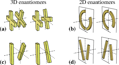
Figure 1: (Color online) (a–b) Schematic illustration and (c–d) plasmonic dimer representation of 3D and 2D enantiomeric meta-atoms.

Another group of unusual physical phenomena in metamaterials results from their ability to transform polarization of light. One example is giant optical activity Kuwata-Gonokami et al. [2005] in composite materials containing spiral-like or otherwise twisted meta-atoms (see, e.g., figure 1a). Recently, planar chiral metamaterials (PCMs) were introduced Potts et al. [2004], Fedotov et al. [2006], Plum et al. [2009] where meta-atoms possess two-dimensional (2D) rather than three-dimensional (3D) enantiomeric asymmetry (figure 1b). While conventional chiral PCMs simply resemble naturally occurring gyrotopic media (e.g., optically active liquids), PCMs are distinct from both 3D chiral and Faraday media in that their polarization eigenstates are co-rotating elliptical rather than counter-rotating elliptical or circular Fedotov et al. [2006], Plum et al. [2009], Zhukovsky et al. [2009]. This leads to exotic polarization properties, e.g., asymmetry in transmission for a forward- vs. backward-propagating circularly polarized incident wave, without nonreciprocity present in Faraday media. Such a rich variety of polarization properties in compact-sized planar structures make chiral metamaterials promising for polarization sensitive integrated optics applications.

Taken generally, the analysis of artificial materials is a complex theoretical and computational problem. In the theoretical research of metamaterials, two areas can roughly be identified. On the one hand, there is the active research concerning various approaches to metamaterial homogenization, i.e., the derivation of macroscopic material parameters (in particular, permittivity and permeability tensors) out of the electromagnetic properties of a single meta-atom Simovski et al. [2002], Smith et al. [2002], Smith and Pendry [2006], Baena et al. [2008]. On the other hand, a lot of effort is invested in the study of light interaction with single nanoparticles (see Myroshnychenko et al. [2008a] and references therein). Metallic (plasmonic) nanoparticles attract special attention Romero [2009] because they can exhibit strong resonances for the wavelengths much larger than their feature sizes.

Both experimentally and theoretically, one typically takes advantage of the scalability of Maxwell’s equations to consider structures with millimeter-scale feature sizes in the microwave and radio-frequency (RF) regime Potts et al. [2004], Fedotov et al. [2006], Plum et al. [2009]. Not only is the metamaterial fabrication on these length scales much easier, but also their theoretical analysis – meta-atoms have a close resemblance to antennas in their ability to connect between propagating radiation and localized near fields. The extensive knowledge in the field of antenna engineering can then be tapped into. Semi-analytical models exist Balanis [1989] that offer insight into field interaction processes in the antennas, and numerical tools for practical antenna design and optimization are well established Volakis [2007].

The optical wavelength range, which is where functional metamaterials attract the most interest, remains far more challenging. At optical frequencies, the metal can no longer be treated as a perfect electric conductor. Because of this fundmental difference the semi-analytical models used in the microwave regime can not be used in the visible and near-infrared spectral range, and the demands in computational resources increase tremendously. Fabrication of metamaterials in the optical domain also remains a challenge because of the small feature sizes (about 10 to 100 nm).

These difficulties notwithstanding, recent progress in nanotechnology have enabled the fabrication of optical antennas (nanoantennas) Bharadwaj et al. [2009], Mühlschlegel et al. [2005] and opened many exciting possibilities towards nanoantenna applications. For example, it has been recently demonstrated that nanoantennas can enhance Rogobete et al. [2007] and direct Taminiau et al. [2008] the emission of single molecules and that they can play a key role in sensing applications Raschke et al. [2003]. Great potential in improving the efficiency of solar cells should also be mentioned Atwater and Polman [2010].

Such a combination of promises and challenges in optical metamaterials creates a strong need for a systematic, ab ibitio, theoretical description of metamaterials, which, on the one hand, would be general enough to span the range of applicable frequencies from RF to optical, and on the other hand, would be simple enough to facilitate the direct prediction of metamaterial properties based on their geometry without having to resort to full-scale numerical simulation in time-consuming adaptive optimization techniques. Such a theoretical description would also be beneficial in order to be able to simplify the geometry of functional (e.g. chiral) meta-atoms so as to facilitate their cost-effective fabrication in the telecommunication and optical domains.

In this paper, we formulate such a theoretical description by investigating the theoretical foundations of light interaction with plasmonic nanoparticles. We start with one metallic particle (a plasmonic monomer) in an external electromagnetic field, and consider the general expression for its susceptibility in terms of the formal Green’s function-based solution of the Maxwell equations. We then set out to simplify this general solution for a nanoparticle of a simple geometry in the approximation of its size being much smaller than the wavelength (the Rayleigh approximation), moving on to the corrections to this approach accounting for the retardation effects. Further we introduce a new semianalytical method to solve the problem of electromagnetic wave scattering on metallic cylindrical wire, which is both accurate and computationally efficient. The results turn out to be equally applicable in the microwave and optical frequency range and can be used for improved designs for plasmonic nanoantennas.

We then apply a similar approach to a pair of closely located nanoparticles (a plasmonic dimer). By accounting for the interaction between the partices in the dimer, we arrive at analytic expressions of the dimer’s polarizability. It is then possible to determine the effective macroscopic parameters of a dilute medium that contains the corresponding dimers as “meta-atoms”. It is shown that dimers of planar geometry without an in-plane mirror symmetry (figure 1d) exhibit crystallographic and spectral properties of planar chiral metamaterials. It is concluded that a geometry as simple as an arrangement of nanorods can support functional metamaterial properties that were previously reported in more intricately shaped meta-atoms.

The structure of the paper is as follows. In Section 2, the systematic approach to single plasmonic particles (monomers) is presented. We start from the general Green’s function solution and review the computational strategies for numerical and semianalytical approaches, ending up with the expressions of effective particle susceptibility (polarizability). In Section 3, a similar approach is applied to plasmonic dimers. The effective polarizability of a dimer is determined and the expressions for effective macroscopic properties such as effective permittivity and permeability is derived. Application of the developed formalism to 2D planar chiral double-rod plasmonic dimers is then presented. Finally, Section 4 summarizes the paper.

2 Plasmonic monomers

2.1 General solution

We describe a nanoparticle by a complex, frequency dependent relative dielectric permittivity $\varepsilon_{r}$. Electric field $\mathbf{E}\left(\mathbf{r}\right)$ in the presence of such a nanoparticle is given by a solution of the homogeneous Helmholtz equation Bladel [2007]

$$\nabla\times\nabla\times\mathbf{E}\left(\mathbf{r}\right)-k^{2}\varepsilon\left(\mathbf{r}\right)\mathbf{E}\left(\mathbf{r}\right)=0.$$ (1)

Here $k=\omega/c$ is a free space wave number and $\varepsilon\left(\mathbf{r}\right)$ is equal to $\varepsilon_{r}$ inside the volume $V$ occupied by the particle and to 1 otherwise. Representing the total field $\mathbf{E}\left(\mathbf{r}\right)=\mathbf{E}^{i}\left(\mathbf{r}\right)+\mathbf{E}^{s}\left(\mathbf{r}\right)$ as a sum of incident $\mathbf{E}^{i}\left(\mathbf{r}\right)$ and scattered $\mathbf{E}^{s}\left(\mathbf{r}\right)$ fields and talking into account that the incident field has to satisfy a free-space Helmholtz equation

$$\nabla\times\nabla\times\mathbf{E}^{i}\left(\mathbf{r}\right)-k^{2}\mathbf{E}^{i}\left(\mathbf{r}\right)=0$$ (2)

one can reformulate the scattering problem (1) in the form of the inhomogeneous Helmholtz equation Bladel [2007]

$$\nabla\times\nabla\times\mathbf{E}^{s}\left(\mathbf{r}\right)-k^{2}\mathbf{E}^{s}\left(\mathbf{r}\right)=\mathrm{i}\omega\mu_{0}\mathbf{j}^{eq}(\mathbf{r})$$ (3)

with an equivalent current density

$$\mathbf{j}^{eq}(\mathbf{r})=-\mathrm{i}\omega\varepsilon_{0}\Delta\varepsilon\left(\mathbf{r}\right)\mathbf{E}(\mathbf{r}),$$ (4)

where $\Delta\varepsilon\left(\mathbf{r}\right)=\varepsilon\left(\mathbf{r}\right)-1$. In this formulation one can clearly see, that the field scattered from a nanoparticle is generated by a current density induced in the particle by the total field $\mathbf{E}\left(\mathbf{r}\right)$.

Taking into account the explicit form of the induced current density (4) a general solution of the inhomogeneous Helmholtz equation (3) can be written as a self-consistent integro-differential equation of the Lippman-Schwinger type Bladel [2007]

$$\mathbf{E}(\mathbf{r})=\mathbf{E}^{i}(\mathbf{r})+k^{2}\left(\overleftrightarrow{\mathbf{I}}+\frac{1}{k^{2}}\nabla\otimes\nabla\right)\\ \int_{V}\mathrm{d}^{3}r^{\prime}g\left(\mathbf{r},\mathbf{r}^{\prime}\right)\Delta\varepsilon\left(\mathbf{r}^{\prime}\right)\mathbf{E}\left(\mathbf{r}^{\prime}\right),$$ (5)

where $\overleftrightarrow{\mathbf{I}}$ denotes the three-dimensional unit tensor, $\otimes$ is the tensor product defined by $\left(\mathbf{a}\otimes\mathbf{b}\right)_{ij}=a_{i}b_{j}$ and

$$g(\mathbf{r},\mathbf{r}^{\prime})=\frac{e^{\mathrm{i}k\left|\mathbf{r}-\mathbf{r}^{\prime}\right|}}{4\pi\left|\mathbf{r}-\mathbf{r}^{\prime}\right|}$$ (6)

is the scalar Green’s function. Denoting the integro-differential operator in (5) by $\overleftrightarrow{\mathbf{t}}$ the Lippman-Schwinger equation can be formally casted in operator notations as

$$\mathbf{E}=\mathbf{E}^{i}+\overleftrightarrow{\mathbf{t}}\mathbf{E}.$$ (7)

To find a general closed-form solution of the Lippman-Schwinger equation (5) we follow here the approach presented in Bozhevolnyi and Lozovski [2000], Bozhevolnyi et al. [2001]. It is well known that one can build a solution of equation (5) in an iterative manner by replacing a self-consistent field in the integral by the field obtained on the left-hand side of the equation at the previous iteration. Starting with the incident field one ends up with an infinite Born series expansion Sheng [2006], which in operator notations reads

$$\mathbf{E}=\mathbf{E}^{i}+\left(\overleftrightarrow{\mathbf{t}}+\overleftrightarrow{\mathbf{t}}^{2}+\overleftrightarrow{\mathbf{t}}^{3}\cdots\right)\mathbf{E}^{i}\\ =\mathbf{E}^{i}+\left(\overleftrightarrow{\mathbf{I}}+\overleftrightarrow{\mathbf{t}}+\overleftrightarrow{\mathbf{t}}^{2}+\cdots\right)\overleftrightarrow{\mathbf{t}}\mathbf{E}^{i}\\ =\mathbf{E}^{i}+\left(\overleftrightarrow{\mathbf{I}}-\overleftrightarrow{\mathbf{t}}\right)^{-1}\overleftrightarrow{\mathbf{t}}\mathbf{E}^{i}$$ (8)

In the last step we have used the formal summation of the operator power series.

It is important to stress here that the Born expansion of a finite order can only be used in the case of relatively weak scattering. In the case of resonant scattering, which is of major importance in nanoplasmonics, finite-order Born approximation will lead to inaccurate results no matter how many terms in the expansion are taken into account Keller et al. [1993]. At the same time, an infinite Born series provides an exact solution of the Lippman-Schwinger problem (5) both in the resonant and the non-resonant case.

The main idea behind finding an exact solution of (5) is to assume that the scattered field $\mathbf{E}^{s}\left(\mathbf{r}\right)$ can be obtained via some dressed integro-differential operator acting on the incident field $\mathbf{E}^{i}\left(\mathbf{r}\right)$ directly Bozhevolnyi and Lozovski [2000], Bozhevolnyi et al. [2001]

$$\mathbf{E}^{s}(\mathbf{r})=\mathbf{E}(\mathbf{r})-\mathbf{E}^{i}(\mathbf{r})=k^{2}\left(\overleftrightarrow{\mathbf{I}}+\frac{1}{k^{2}}\nabla\otimes\nabla\right)\\ \int_{V}\mathrm{d}^{3}r^{\prime}g\left(\mathbf{r},\mathbf{r}^{\prime}\right)\overleftrightarrow{\Xi}\left(\mathbf{r}^{\prime}\right)\Delta\varepsilon\left(\mathbf{r}^{\prime}\right)\mathbf{E}^{i}\left(\mathbf{r}^{\prime}\right)$$ (9)

or in operator notations

$$\mathbf{E}=\mathbf{E}^{i}+\overleftrightarrow{\mathbf{T}}\mathbf{E}^{i}.$$ (10)

Here the unknown tensor $\overleftrightarrow{\Xi}\left(\mathbf{r}\right)$ has to be determined. Comparing relation (10) with the last line of relation (8) it can be immediately recognized that the dressed operator $\overleftrightarrow{\mathbf{T}}$ must satisfy the Dyson-like equation

$$\overleftrightarrow{\mathbf{T}}=\overleftrightarrow{\mathbf{t}}+\overleftrightarrow{\mathbf{T}}\overleftrightarrow{\mathbf{t}}.$$ (11)

To find an unknown tensor $\overleftrightarrow{\Xi}\left(\mathbf{r}\right)$ we act with the operator (11) on an arbitrary plane harmonic incident field $\mathbf{E}^{i}\left(\mathbf{r}\right)=\mathbf{E}_{0}\exp\left(\mathrm{i}\mathbf{k}\cdot\mathbf{r}\right)$, where $\mathbf{k}$ is the wave vector and $\mathbf{E}_{0}$ the amplitude of the incident field. This leads after a few simple steps to the following integro-differential equation for the unknown tensor $\overleftrightarrow{\Xi}$

$$k^{2}\left(\overleftrightarrow{\mathbf{I}}+\frac{1}{k^{2}}\nabla\otimes\nabla\right)\int_{V}\mathrm{d}^{3}r^{\prime}\\ \biggl{\{}\left(\overleftrightarrow{\Xi}\left(\mathbf{r}^{\prime}\right)g\left(\mathbf{r},\mathbf{r}^{\prime}\right)\Delta\varepsilon\left(\mathbf{r}^{\prime}\right)-g\left(\mathbf{r},\mathbf{r}^{\prime}\right)\Delta\varepsilon\left(\mathbf{r}^{\prime}\right)\right)\mathrm{e}^{\mathrm{i}\mathbf{k}\cdot\mathbf{r}^{\prime}}-\\ \overleftrightarrow{\Xi}\left(\mathbf{r}^{\prime}\right)g\left(\mathbf{r},\mathbf{r}^{\prime}\right)\Delta\varepsilon\left(\mathbf{r}^{\prime}\right)k^{2}\left(\overleftrightarrow{\mathbf{I}}+\frac{1}{k^{2}}\nabla^{\prime}\otimes\nabla^{\prime}\right)\int_{V}\mathrm{d}^{3}r^{\prime\prime}\\ g\left(\mathbf{r}^{\prime},\mathbf{r}^{\prime\prime}\right)\Delta\varepsilon\left(\mathbf{r}^{\prime\prime}\right)\mathrm{e}^{\mathrm{i}\mathbf{k}\cdot\mathbf{r}^{\prime\prime}}\biggr{\}}\mathbf{E}_{0}=0.$$ (12)

Since the amplitude of the incident field $\mathbf{E}_{0}$ can be arbitrary, the integral in this equation can be zero only for a vanishing integrand. That means that the expression in the curly brackets should be equal to zero leading to

$$\overleftrightarrow{\Xi}\left(\mathbf{r}^{\prime}\right)-\overleftrightarrow{\mathbf{I}}-\overleftrightarrow{\Xi}\left(\mathbf{r}^{\prime}\right)k^{2}\left(\overleftrightarrow{\mathbf{I}}+\frac{1}{k^{2}}\nabla^{\prime}\otimes\nabla^{\prime}\right)\\ \int_{V}\mathrm{d}^{3}r^{\prime\prime}g\left(\mathbf{r}^{\prime},\mathbf{r}^{\prime\prime}\right)\Delta\varepsilon\left(\mathbf{r}^{\prime\prime}\right)\mathrm{e}^{\mathrm{i}\,\mathbf{k}\cdot\left(\mathbf{r}^{\prime\prime}-\mathbf{r}^{\prime}\right)}=0.$$ (13)

This equation can be easily solved to find the unknown tensor

$$\overleftrightarrow{\Xi}\left(\mathbf{r}\right)=\left(\overleftrightarrow{\mathbf{I}}-\overleftrightarrow{\Sigma}\left(\mathbf{r}\right)\right)^{-1}$$ (14)

where

$$\overleftrightarrow{\Sigma}\left(\mathbf{r}\right)=k^{2}\left(\overleftrightarrow{\mathbf{I}}+\frac{1}{k^{2}}\nabla\otimes\nabla\right)\int_{V}\mathrm{d}^{3}r^{\prime}\\ g\left(\mathbf{r},\mathbf{r}^{\prime}\right)\Delta\varepsilon\left(\mathbf{r}^{\prime}\right)\mathrm{e}^{\mathrm{i}\mathbf{k}\cdot\left(\mathbf{r}^{\prime}-\mathbf{r}\right)}$$ (15)

plays the role of a self-energy operator. With tensor $\overleftrightarrow{\Xi}\left(\mathbf{r}\right)$ found, equation (9) gives an exact closed-form solution of the Lippman-Schwinger equation (5).

It is instructive to reformulate this solution slightly. Recalling that $\Delta\varepsilon\left(\mathbf{r}\right)=\varepsilon\left(\mathbf{r}\right)-1$ and $\varepsilon\left(\mathbf{r}\right)=\chi\left(\mathbf{r}\right)+1$, where $\chi\left(\mathbf{r}\right)$ is the electric susceptibility, one can rewrite the exact solution (9) in the following form

$$\mathbf{E}(\mathbf{r})=\mathbf{E}^{i}(\mathbf{r})+k^{2}\left(\overleftrightarrow{\mathbf{I}}+\frac{1}{k^{2}}\nabla\otimes\nabla\right)\int_{V}\mathrm{d}^{3}r^{\prime}\\ g\left(\mathbf{r},\mathbf{r}^{\prime}\right)\overleftrightarrow{\mathrm{X}}\left(\mathbf{r}^{\prime}\right)\mathbf{E}^{i}\left(\mathbf{r}^{\prime}\right),$$ (16)

where an effective susceptibility tensor of a nanoparticle $\overleftrightarrow{\mathrm{X}}\left(\mathbf{r}\right)=\chi\left(\mathbf{r}\right)\overleftrightarrow{\Xi}\left(\mathbf{r}\right)$ was introduced. Please note that such a general solution is a solution of the inhomogeneous Helmholtz equation with the equivalent current density

$$\mathbf{j}^{eq}(\mathbf{r})=-\mathrm{i}\omega\varepsilon_{0}\overleftrightarrow{\mathrm{X}}\left(\mathbf{r}\right)\mathbf{E}^{i}(\mathbf{r}),$$ (17)

which justifies the interpretation of $\overleftrightarrow{\mathrm{X}}\left(\mathbf{r}\right)$ as an effective susceptibility tensor connecting an induced linear polarization $\mathbf{P}\left(\mathbf{r}\right)=\varepsilon_{0}\overleftrightarrow{\mathrm{X}}\left(\mathbf{r}\right)\mathbf{E}^{i}(\mathbf{r})$ of the particle with the incident field $\mathbf{E}^{i}\left(\mathbf{r}\right)$. In this formulation one can immediately recognize that in the case of the resonant scattering the integral in (16) will be defined by the poles of the effective susceptibility

$$\overleftrightarrow{\mathrm{X}}\left(\mathbf{r}\right)=\chi\left(\mathbf{r}\right)\left(\overleftrightarrow{\mathbf{I}}-\overleftrightarrow{\Sigma}\left(\mathbf{r}\right)\right)^{-1}$$ (18)

as it is required within the linear response theory approach Abrikosov A. A. [1965].

The integrals in (15) and (16) are improper at $\mathbf{r}=\mathbf{r}^{\prime}$ due to a singularity of the scalar Green’s function. Consequently one cannot calculate an effective susceptibility without an appropriate regularization. To extract the singularity, one can exclude an arbitrary principal volume $V^{*}$ around the singular point $\mathbf{r}$, and proceed as in Lee et al. [1980] to express (18) in the regularized form

$$\overleftrightarrow{\Sigma}\left(\mathbf{r}\right)=k^{2}\left\{\int_{V-V^{\star}}\mathrm{d}^{3}r^{\prime}\overleftrightarrow{\mathbf{G}}(\mathbf{r},\mathbf{r}^{\prime})\chi\left(\mathbf{r}^{\prime}\right)\mathrm{e}^{\mathrm{i}\mathbf{k}\cdot\left(\mathbf{r}^{\prime}-\mathbf{r}\right)}\right.+\\ \int_{V^{\star}}\mathrm{d}^{3}r^{\prime}\biggl{[}\overleftrightarrow{\mathbf{G}}(\mathbf{r},\mathbf{r}^{\prime})\chi\left(\mathbf{r}^{\prime}\right)\mathrm{e}^{\mathrm{i}\mathbf{k}\cdot\left(\mathbf{r}^{\prime}-\mathbf{r}\right)}-\\ \frac{1}{k^{2}}\left(\nabla\cdot\left[\nabla g_{0}(\mathbf{r},\mathbf{r}^{\prime})\right]\right)\chi\left(\mathbf{r}\right)\biggr{]}\left.-\frac{1}{k^{2}}\overleftrightarrow{\mathbf{L}}_{V^{*}}\chi\left(\mathbf{r}\right)\right\},$$ (19)

where $\overleftrightarrow{\mathbf{G}}(\mathbf{r},\mathbf{r}^{\prime})$ is the dyadic Green’s function

$$\overleftrightarrow{\mathbf{G}}(\mathbf{r},\mathbf{r}^{\prime})=\left(\overleftrightarrow{\mathbf{I}}+\frac{1}{k^{2}}\nabla\otimes\nabla\right)g(\mathbf{r},\mathbf{r}^{\prime}),$$ (20)

and $g_{0}$ is the static Green’s function

$$g_{0}(\mathbf{r},\mathbf{r}^{\prime})=\lim_{k\rightarrow 0}g(\mathbf{r},\mathbf{r}^{\prime})=\frac{1}{4\pi}\frac{1}{\left|\mathbf{r}-\mathbf{r}^{\prime}\right|}.$$ (21)

$\overleftrightarrow{\mathbf{L}}_{V^{*}}$ denotes the source dyadic

$$\overleftrightarrow{\mathbf{L}}_{V^{*}}=\frac{1}{4\pi}\oint_{\partial V^{\star}}\mathrm{d}^{2}r^{\prime}\frac{\mathbf{R}\otimes\hat{\mathbf{n}}}{R^{3}}$$ (22)

which accounts for the depolarization of the excluded volume $V^{\star}$ and depends entirely on the geometry of the principal volume, but does not depend on its size or position Yaghjian [1980]. Here $\mathbf{R}=\mathbf{r}^{\prime}-\mathbf{r}$, $R=\left|\mathbf{R}\right|$, $\partial V^{\star}$ is a surface enclosing principal volume $V^{*}$ and $\hat{\mathbf{n}}$ is its outward unit normal. The dyadic Green’s function defined in (20) can be calculated explicitly and is equal to

$$\overleftrightarrow{\mathbf{G}}(\mathbf{r},\mathbf{r}^{\prime})=\frac{e^{\mathrm{i}kR}}{4\pi R}\left\{\left(1+\frac{\mathrm{i}kR-1}{k^{2}R^{2}}\right)\overleftrightarrow{\mathbf{I}}\right.+\\ \left.\frac{3-3\mathrm{i}kR-k^{2}R^{2}}{k^{2}R^{2}}\frac{\mathbf{R}\otimes\mathbf{R}}{R^{2}}\right\}$$ (23)

For points inside the particle , the integral in (16) can be regularized in the similar fashion, resulting in

$$\mathbf{E}(\mathbf{r})=\mathbf{E}^{i}(\mathbf{r})+k^{2}\left\{\int_{V-V^{\star}}\mathrm{d}^{3}r^{\prime}\overleftrightarrow{\mathbf{G}}(\mathbf{r},\mathbf{r}^{\prime})\overleftrightarrow{\mathrm{X}}\left(\mathbf{r}^{\prime}\right)\mathbf{E}^{i}\left(\mathbf{r}^{\prime}\right)\right.+\\ \int_{V^{\star}}\mathrm{d}^{3}r^{\prime}\biggl{[}\overleftrightarrow{\mathbf{G}}(\mathbf{r},\mathbf{r}^{\prime})\overleftrightarrow{\mathrm{X}}\left(\mathbf{r}^{\prime}\right)\mathbf{E}^{i}\left(\mathbf{r}^{\prime}\right)-\\ \frac{1}{k^{2}}\left(\nabla\cdot\left[\nabla g_{0}(\mathbf{r},\mathbf{r}^{\prime})\right]\right)\overleftrightarrow{\mathrm{X}}\left(\mathbf{r}\right)\mathbf{E}^{i}\left(\mathbf{r}\right)\biggr{]}\\ \left.-\frac{1}{k^{2}}\overleftrightarrow{\mathbf{L}}_{V^{*}}\overleftrightarrow{\mathrm{X}}\left(\mathbf{r}\right)\mathbf{E}^{i}\left(\mathbf{r}\right)\right\}.$$ (24)

For points outside the particle general solution is given by

$$\mathbf{E}(\mathbf{r})=\mathbf{E}^{i}(\mathbf{r})+k^{2}\int_{V}\mathrm{d}^{3}r^{\prime}\overleftrightarrow{\mathbf{G}}(\mathbf{r},\mathbf{r}^{\prime})\overleftrightarrow{\mathrm{X}}\left(\mathbf{r}^{\prime}\right)\mathbf{E}^{i}\left(\mathbf{r}^{\prime}\right).$$ (25)

2.2 Rayleigh approximation

If the nanoparticle dimensions are much smaller than the incident light wavelength, the scattering problem (5) can be treated within a quasi-static limit $\left|\mathbf{k}\right|=0$. Letting the principal volume to be infinitesimal, the regularized integral in (19) can be reduced to Karam [1997]

$$\overleftrightarrow{\Sigma}=-\frac{\chi_{r}}{4\pi}\oint_{\partial V}\mathrm{d}^{2}r^{\prime}\frac{\mathbf{R}\otimes\hat{\mathbf{n}}}{R^{3}}=-\chi_{r}\overleftrightarrow{\mathbf{L}}.$$ (26)

Here the susceptibility of the particle $\chi_{r}$ is taken outside of the integral, while it is assumed to be constant inside the particle. The integration is performed over the particle surface $\partial V$. In (26) we have introduced the depolarization tensor of the particle $\overleftrightarrow{\mathbf{L}}$. This tensor depends solely on the particle shape.

Taking into account (26) one obtains a quasi-static effective susceptibility of the small particle in the form

$$\overleftrightarrow{\mathrm{X}}=\chi_{r}\left(\overleftrightarrow{\mathbf{I}}+\chi_{r}\overleftrightarrow{\mathbf{L}}\right)^{-1}.$$ (27)

The field induced in the particle is given by the quasi-static limit of (24)

$$\mathbf{E}(\mathbf{r})=\mathbf{E}^{i}-\overleftrightarrow{\mathbf{L}}\overleftrightarrow{\mathrm{X}}\mathbf{E}^{i},$$ (28)

which, taking into account that the depolarization tensor is symmetric Yaghjian [1980], can be combined with (27) to obtain the familiar relation for the electric field in the Rayleigh approximation

$$\mathbf{E}(\mathbf{r})=\left(\overleftrightarrow{\mathbf{I}}+\chi_{r}\overleftrightarrow{\mathbf{L}}\right)^{-1}\mathbf{E}^{i}.$$ (29)

Further we calculate the effective quasi-static susceptibility for a small metallic nanoparticle. Taking into account that the depolarization tensor is symmetric, the effective susceptibility (27) can be written in component form as

$$\overleftrightarrow{\mathrm{X}}=\frac{\chi_{r}}{1+\chi_{r}L_{ii}}\mathbf{\hat{x}}_{i}\otimes\mathbf{\hat{x}}_{i},$$ (30)

where $\mathbf{\hat{x}}_{i}$ are the unit vectors along the main particle axes. Assuming for simplicity the Drude model for the metal

$$\chi_{r}=-\frac{\omega_{p}^{2}}{\omega^{2}+\mathrm{i}\gamma\omega},$$ (31)

with $\omega_{p}$ being the plasma frequency and $\gamma$ being the damping rate, the relation (30) results in

$$\overleftrightarrow{\mathrm{X}}=\frac{\omega_{p}^{2}}{\omega_{p}^{2}L_{ii}-\omega^{2}-\mathrm{i}\gamma\omega}\mathbf{\hat{x}}_{i}\otimes\mathbf{\hat{x}}_{i}.$$ (32)

Then the polarization of the metallic particle $\mathbf{P}=\varepsilon_{0}\overleftrightarrow{\mathrm{X}}\mathbf{E}^{i}$ for an arbitrary plane harmonic incident field $\mathbf{E}^{i}$ should satisfy the following algebraic equation

$$-\omega^{2}\mathbf{P}-\mathrm{i}\gamma\omega\mathbf{P}+\omega_{p}^{2}L_{ii}\mathbf{P}=\varepsilon_{0}\omega_{p}^{2}\mathbf{\hat{x}}_{i}\otimes\mathbf{\hat{x}}_{i}\mathbf{E}^{i},$$ (33)

which after taking an inverse Fourier transform results in the dynamic equation for a harmonic, damped, driven oscillator

$$\frac{\mathrm{d}^{2}\mathbf{P}}{\mathrm{d}t^{2}}+\gamma\frac{\mathrm{d}\mathbf{P}}{\mathrm{d}t}+\omega_{0}\mathbf{P}=\varepsilon_{0}\omega_{p}^{2}\mathbf{\hat{x}}_{i}\otimes\mathbf{\hat{x}}_{i}\mathbf{E}^{i}$$ (34)

with the resonance frequency $\omega_{0}=\omega_{p}^{2}L_{ii}$ defined by the particle material and shape. Such collective oscillations of the electron plasma confined to the metallic particle corresponds to a particle plasmon-polariton excitation.

2.3 Retardation

With increasing particle size the retardation effects become important and to obtain an effective susceptibility of the particle as well as associated scattered field one has to calculate the integrals in (15) and (16) explicitly. To do that, one should choose the principal volume carefully. Technically the form and the size of the principal volume can be arbitrary Lee et al. [1980]. In order to recover the quasi-static limit it is convenient to choose the principal volume similar in shape to the considered particle. Furthermore, the principal volume can be chosen infinitesimally small, resulting in the following exact solution of the scattering problem for the points inside the particle:

$$\mathbf{E}(\mathbf{r})=\mathbf{E}^{i}(\mathbf{r})+k^{2}\int_{V-V^{\star}}\mathrm{d}^{3}r^{\prime}\\ \overleftrightarrow{\mathbf{G}}(\mathbf{r},\mathbf{r}^{\prime})\overleftrightarrow{\mathrm{X}}\left(\mathbf{r}^{\prime}\right)\mathbf{E}^{i}\left(\mathbf{r}^{\prime}\right)-\overleftrightarrow{\mathbf{L}}\overleftrightarrow{\mathrm{X}}\left(\mathbf{r}\right)\mathbf{E}^{i}\left(\mathbf{r}\right)$$ (35)

with the self-energy tensor given by

$$\overleftrightarrow{\Sigma}\left(\mathbf{r}\right)=k^{2}\int_{V-V^{\star}}\mathrm{d}^{3}r^{\prime}\\ \overleftrightarrow{\mathbf{G}}(\mathbf{r},\mathbf{r}^{\prime})\chi\left(\mathbf{r}^{\prime}\right)\mathrm{e}^{\mathrm{i}\mathbf{k}\cdot\left(\mathbf{r}^{\prime}-\mathbf{r}\right)}-\overleftrightarrow{\mathbf{L}}\chi\left(\mathbf{r}\right).$$ (36)

Note that in (35) and (36) $\overleftrightarrow{\mathbf{L}}$ is the depolarization tensor of the particle and the infinitesimal principal volume $V^{*}$ has to have the same shape as the particle under consideration.

Denoting the result of the integration in (36) by $\overleftrightarrow{\mathbf{D}}\left(\mathbf{r}\right)$ one obtains the effective susceptibility of the particle

$$\overleftrightarrow{\mathrm{X}}\left(\mathbf{r}\right)=\chi_{r}\left(\overleftrightarrow{\mathbf{I}}+\chi_{r}\overleftrightarrow{\mathbf{L}}-\overleftrightarrow{\mathbf{D}}\left(\mathbf{r}\right)\right)^{-1}.$$ (37)

Spatial and frequency dependence of the effective susceptibility originated from the field retardation is contained in the dynamic depolarization tensor $\overleftrightarrow{\mathbf{D}}\left(\mathbf{r}\right)$.

To estimate the main effect of the field retardation on the effective susceptibility tensor we evaluate the dynamic depolarization tensor. The following approximations are used to simplify the analysis. First, we assume that the phase difference due to the incident field is negligible within the particle, i.e., $\exp\left(\mathrm{i}\mathbf{k}\cdot\left(\mathbf{r}^{\prime}-\mathbf{r}\right)\right)\approx 1$ in (36). Second, we use only the first few terms in the long-wavelength expansion of the dyadic Green’s function in powers of $k$ to calculate the integral

$$k^{2}\overleftrightarrow{\mathbf{G}}(\mathbf{r},\mathbf{r}^{\prime})\approx\frac{1}{4\pi}\left(-\frac{\overleftrightarrow{\mathbf{I}}}{R^{3}}+3\frac{\mathbf{R}\otimes\mathbf{R}}{R^{5}}\right)+\\ \frac{k^{2}}{8\pi}\left(\frac{\overleftrightarrow{\mathbf{I}}}{R}+\frac{\mathbf{R}\otimes\mathbf{R}}{R^{3}}\right)+\frac{\mathrm{i}k^{3}}{6\pi}\overleftrightarrow{\mathbf{I}}.$$ (38)

Finally, we use the mean value theorem to approximate the resulting integral by its value in the geometrical center of the particle.

For a centrosymmetric particle, e.g., a sphere, a regular cylinder, or a block, the integral of the first term in (38) is equal to zero, the second term results in some symmetric shape-dependent tensor $k^{2}V\overleftrightarrow{\mathbf{D}}^{\prime}$, while the integral over the last term results in $\mathrm{i}k^{3}(V/6\pi)\overleftrightarrow{\mathbf{I}}$. This leads to the following form of the dynamic depolarization tensor

$$\overleftrightarrow{\mathbf{D}}\left(\mathbf{r}\right)=k^{2}V\overleftrightarrow{\mathbf{D}}^{\prime}+\mathrm{i}k^{3}\frac{V}{6\pi}\overleftrightarrow{\mathbf{I}}.$$ (39)

Taking into account that this dynamic depolarization tensor is symmetric, the effective susceptibility (27) can be written in component form as

$$\overleftrightarrow{\mathrm{X}}=\frac{\chi_{r}}{1+\chi_{r}L_{ii}-k^{2}VD_{ii}^{\prime}-\mathrm{i}k^{3}\frac{V}{6\pi}}\mathbf{\hat{x}}_{i}\otimes\mathbf{\hat{x}}_{i},$$ (40)

which for metallic nanoparticle described by the Drude model (31) leads to the following equation for the induced polarization

$$-\omega^{2}\mathbf{P}-\mathrm{i}\gamma\omega\mathbf{P}+\omega_{p}^{2}L_{ii}\mathbf{P}+\omega^{4}\frac{V}{c^{2}}\left(D_{ii}^{\prime}-\frac{\gamma}{6\pi c}\right)\mathbf{P}+\\ \mathrm{i}\omega^{3}\frac{\gamma VD_{ii}^{\prime}}{c^{2}}\mathbf{P}+\mathrm{i}\omega^{5}\frac{V}{6\pi c^{3}}\mathbf{P}=\varepsilon_{0}\omega_{p}^{2}\mathbf{\hat{x}}_{i}\otimes\mathbf{\hat{x}}_{i}\mathbf{E}^{i}.$$ (41)

Taking the inverse Fourier transform results in

$$\frac{\mathrm{d}^{2}\mathbf{P}}{\mathrm{d}t^{2}}+\gamma\frac{\mathrm{d}\mathbf{P}}{\mathrm{d}t}+\omega_{0}\mathbf{P}+\\ \gamma_{3}\frac{\mathrm{d}^{3}\mathbf{P}}{\mathrm{d}t^{3}}+\omega_{4}\frac{\mathrm{d}^{4}\mathbf{P}}{\mathrm{d}t^{4}}-\gamma_{5}\frac{\mathrm{d}^{5}\mathbf{P}}{\mathrm{d}t^{5}}=\varepsilon_{0}\omega_{p}^{2}\mathbf{\hat{x}}_{i}\otimes\mathbf{\hat{x}}_{i}\mathbf{E}^{i},$$ (42)

which describes an anharmonic, damped, driven oscillator. Parameters $\omega_{0}$, $\omega_{4}$, $\gamma_{3}$ and $\gamma_{5}$ can be easily deduced from the comparison of equations (41) and (42). As can be clearly seen from equation (42), retardation leads (i) to anharmonicity and as a consequence to a shift of the resonance frequency (frequency of the particle plasmon-polariton) and (ii) to additional radiation damping, which broaden the resonance itself.

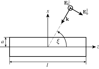
Figure 2: Definition of the geometrical parameters, radius $a$ and length $l$, of the scattering cylinder as well as the chosen body centered coordinate system. Additionally the incident angle $\xi$ and the polarization basis vector $\mathbf{E}_{0}^{\parallel}$ are depicted in the incident plane.

Figure 3: Comparison of the scattering cross section for scattering normal incident light on a gold cylinder (radius 10 nm, length 100 nm) calculated using the Rayleigh susceptibility (dashed) and the retarded susceptibility (solid).

In figure 3 the total scattering cross section for normal incident light scattered on a regular gold nanocylinder is shown. The geometry of the problem is depicted in figure 2. The following parameter are used for calculations, particle radius is $a=10$ nm and its length is $l=100$ nm. The relative permittivity of gold is modeled by a free electron Drude-Sommerfeld model

$$\varepsilon_{r}(\omega)\approx\epsilon_{\infty}-\frac{\omega_{p}^{2}}{\omega^{2}+i\gamma\omega}$$ (43)

with $\varepsilon_{\infty}=9$, $\omega_{p}=1.36674\cdot 10^{16}\,s^{-1}$ and $\gamma=7.59297\cdot 10^{13}\,s^{-1}$ (see Myroshnychenko et al. [2008b]). Figure 3 shows both the scattering cross section obtained from the effective susceptibility (27) within the Rayleigh approximation (dashed line) and from the retarded effective susceptibility (40). One can clearly see that retardation results in a resonance frequency shift towards lower frequencies and to a broadening of the resonance peak.

2.4 Numerical solutions

To obtain a more rigorous solution of the scattering problem, direct numerical methods have to be used. One class of methods discretize the volume integral equation, that is equation (35) with the replacement $\overleftrightarrow{\mathrm{X}}\left(\mathbf{r}^{\prime}\right)\mathbf{E}^{i}\left(\mathbf{r}^{\prime}\right)\rightarrow\mathbf{E}(\mathbf{r}^{\prime})$. A popular representative of this class of solvers is the discrete dipole approximation (DDA) Yurkin and Hoekstra [2007] which solves for induced dipole moments of small cubes in which the scatterer is decomposed. A numerical method also based on an integral solution of Maxwell’s equation but expressed in terms of surface instead of volume integrals is the boundary element method (BEM) Myroshnychenko et al. [2008c]. An advantage of integral equation based methods compared with direct solutions of Maxwell’s equations is that only the scatterer has to be discretized, in BEM actually just its surface, and one does not have to deal with unwanted reflections at the borders of the computational domains. The approach of solving Maxwell’s equation in the frequency domain directly on a volumetric unstructured mesh is called the finite element method (FEM) Jin [2002]. The idea in FEM is to approximate the electromagnetic field by polynomials of low order on each small mesh volume. Plugging this test functions into Maxwell’s equation together with boundary and connection conditions, one yields a system of linear equations to be solved Jin [2002]. Similar in both the basic idea and mesh type but formulated in time domain is the discontinuous Galerkin time domain method (DGTD) Stannigel et al. [2009], Hesthaven [2002]. Another very popular time domain method is the finite-difference time-domain (FDTD) method Taflove and Hagnes [2000]. Formulated on a structured Cartesian grid and approximating the spatial and time derivatives by central differences, this algorithm is explicit, i.e., no set of linear equations has to be solved. Therefore the implementation of the method is relatively simple and numerical stability is not a concern as long as space and time discretization are connected by the Courant relation Taflove and Hagnes [2000]. On the downside one has to mention that one has to choose a very small space discretization to accurately describe curved surfaces of scatterers which leads to high memory consumption and long computation times.

In figure 4 the total scattering cross section calculated with different direct numerical methods is depicted for scattering of a plane wave under slanting incidence ($\xi=\frac{\pi}{4}$) on a gold nanowire with radius $a=10nm$ and length $l=200nm$ (see figure 2). Gold is described by the equation (43) with the associated parameters. The numerical methods and their implementations are, in particular: (i) adda, an open source DDA implementation Yurkin et al. [2007] (solid line); (ii) HFSS, a commercial FEM frequency domain solver from Ansys Inc.Ansys (dashed line); and (iii) a self-implemented FDTD code (dotted line). The two panels a) and b) show the first and third resonance peak respectively. The space discretization in both the DDA and FDTD calculation (both methods use a cartesian voxel mesh) was set to 1 nm which leads to reasonable convergence. The mesh in HFSS is created by an adaptive algorithm so that there is no uniform discretization step. As basis functions second order polynomials are used. The execution time of DDA and HFSS per frequency point was about 8 and 6 minutes on one core of a modern workstation, respectively. The given execution time of HFSS has taken into account the adaptive recreation of the computational mesh for each of the depicted panels. FDTD, due to its time domain roots, yields the whole spectrum in one run which needs about 250 minutes. As it can be seen in figure 4 the agreement between the different numerical method are reasonable but not perfect despite high accuracy in sampling and long execution times.

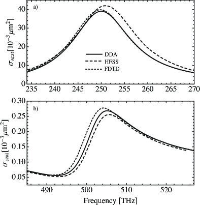
Figure 4: Scattering cross-section of a gold nanowire ($l=200\text{ nm},\,a=10\text{ nm}$) under slanting incidence ($\xi=\frac{\pi}{4}$) calculated with different rigorous numerical methods. In the top panel (a) the first and in the bottom panel (b) the third resonance peak are shown.

2.5 Semi-analytical methods

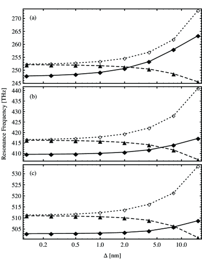
Figure 5: Convergence of the first three resonances (from top to bottom panel) of a gold nanowire ($l=200\text{ nm},\,a=10\text{ nm}$) under slanting incidence ($\xi=\frac{\pi}{4}$) calculated with VC-IE method (solid line), SI-IE method (dashed) and Hallen’s method (dotted).

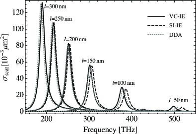
Figure 6: Scattering cross-sections of gold nanowire with fixed radius $a=10$ nm and different lengths. The full and dashed lines show the VC and SI integral equation results, respectively. The dotted line is the numerically rigorous reference calculated using a DDA method Kremers and Chigrin [2011].

To overcome the dependence on time consuming numerical simulations we propose some semi-analytical methods to calculate the scattering of an incident plane wave on a cylindrical wire as depicted in figure 2. Further we assume that the radius $a$ of the wire is small compared with the wavelength of the incident light (electrically thin wire). In this case the incident light interacting with the wire can be regarded as a function of $z$ alone

$$\mathbf{E}^{i}(\mathbf{r}) \approx \mathbf{E}_{0}^{\parallel}e^{-ikz\cos\xi}$$ (44)

where $\mathbf{E}_{0}^{\parallel}$ denotes the field component along the wire axis. First we briefly review how the scattering problem is solved in microwave and RF spectral regime. In this spectral regime metals can be treated as perfect electric conductor (PEC) with the consequence that the induced current density has just a longitudinal $z$-component residing on the wire interface. Expressed in terms of the total current $I$ the induced current density in this case can be written as

$$\mathbf{j}(\mathbf{r})=\hat{\mathbf{z}}I(z)\frac{\delta(\rho-a)}{2\pi a}$$ (45)

By using (45) in the Lippman-Schwinger equation (5) instead of the equivalent current density (4) one derives the integro-differential equation

$$E_{z}(a,z)=E_{z}^{inc}(z)+i\frac{\omega\mu_{0}}{2\pi}\left(1+\frac{1}{k^{2}}\frac{\partial^{2}}{\partial z^{2}}\right)\\ \int_{-\frac{l}{2}}^{\frac{l}{2}}dz^{\prime}\int_{0}^{2\pi}d\phi^{\prime}\,g_{a}(\phi^{\prime},z-z^{\prime})I(z^{\prime})$$ (46)

where $g_{a}(\phi^{\prime},z-z^{\prime})=g(\mathbf{r},\mathbf{r}^{\prime})$ with $\mathbf{r}=\left(a,0,z\right)$ and $\mathbf{r}^{\prime}=\left(a,\phi^{\prime},z^{\prime}\right)$ in cylindrical coordinates. For a perfect electric conductor the tangential electric field at the wire interface, $E_{z}(a,z)$, vanishes and (46) reduces to the well known Pocklington integro-differential equation Orfanidis [2010]. In the optical and near-infrared spectral regime metals exhibit finite conductivity and a skin depth of the order of typical dimensions of plasmonic particles. However, as long as the wire is thin, regarding the induced current as pure surface current should still be a plausible ansatz. In contrast, vanishing tangential electric field $E_{z}(a,z)$ can not be accepted for wires with finite conductivity. So one approach to derive a self-consistent equation to determine $I$ is to express the left hand side of (46) in terms of the current $I$ by utilizing the known exact solution of the plane wave scattering problem on an infinite cylinder Bohren and Huffman [1998]. This should work reasonably well for wires with high aspect ratio, i.e. $l\gg a$. The analytical solution shows that the electric field inside an infinitely long, electrically thin cylinder under plane wave incidence can be approximated with high accuracy by

$$\mathbf{E}(\mathbf{r})\approx\hat{\mathbf{z}}f(z)J_{0}\left(k_{\rho}\rho\right)$$ (47)

with $J_{0}$ being the Bessel function of the first kind of 0-th order and $k_{\rho}=k\sqrt{\varepsilon_{r}-\cos^{2}\xi}$. From this expression one can derive a relation between the current and the surface electric field as

$$E_{z}(a,z)=Z_{S}I(z)$$ (48)

with the surface impedance

$$Z_{S}=i\frac{J_{0}(k_{\rho}a)k_{\rho}}{2\pi a\omega\epsilon_{0}\Delta\epsilon_{r}J_{1}(k_{\rho}a)}.$$ (49)

Relation (48) can now be used to express the surface field on the left-hand side of (46) in terms of the current $I$. This yields a self-consistent surface impedance (SI) integro-differential equation Hanson [2006]

$$Z_{S}I(z)=E_{z}^{inc}(z)+i\frac{\omega\mu_{0}}{2\pi}\left(1+\frac{1}{k^{2}}\frac{\partial^{2}}{\partial z^{2}}\right)\\ \int_{-\frac{l}{2}}^{\frac{l}{2}}dz^{\prime}\int_{0}^{2\pi}d\phi^{\prime}\,g_{a}(\phi^{\prime},z-z^{\prime})I(z^{\prime})$$ (50)

suitable to calculate the current in thin wires with high aspect ratios and finite conductivity. However, a more consistent treatment is possible. One can directly use (47) as an ansatz for the electric field in (46) on both sides. The result we obtain is the volume current (VC) integro-differential equation

$$f(z)J_{0}\left(k_{\rho}a\right)=E_{z}^{inc}(z)+k^{2}\Delta\epsilon_{r}\left(1+\frac{1}{k^{2}}\frac{\partial^{2}}{\partial z^{2}}\right)\\ \int_{V}d^{3}r^{\prime}\,g(a,z;\mathbf{r}^{\prime})f(z^{\prime})J_{0}\left(k_{\rho}\rho^{\prime}\right)$$ (51)

which determines the amplitude function $f(z)$.

Both in equation (50) and in (51) the differential operator $1+k^{-2}\partial_{z}^{2}$ can be brought inside the integral by means of Lee’s regularization Lee et al. [1980] already used in (24). We thus get rid of the necessity to impose additional boundary conditions. The regularization step is strictly speaking not needed in case of the SI integro-differential equation (50) because it can also be solved in its present form by Hallen’s approach Orfanidis [2010] using the boundary conditions $I(z)=0$ for $z=-l/2$ and $z=l/2$. However, using pure integral equation is the preferred way because $I(z)$ is discontinuous at the wire tips so that enforcing the current to vanish at the wire ends leads to bad convergence when solving (50) numerically. In contrast the VC integro-differential equation can not be solved in its present form (51) because we do not know appropriate boundary conditions for the electric field at the tips. After regularization both the SI-IE and VC-IE can be discretized within a point matching method of moments (MoM) scheme Orfanidis [2010]. This leads to an $n$-dimensional matrix equations in the form

$$\mathbf{U}=\left(\Gamma\overleftrightarrow{\mathbf{I}}-\overleftrightarrow{\mathbf{M}}\right)^{-1}\mathbf{E}_{z}^{i}$$ (52)

where the dimensionality $n$ is the number of slices in which the wire is divided. The $i$-th component of $\mathbf{U}$ denotes the unknown function values $I(z_{i})$ and $f(z_{i})$ at the discrete point $z_{i}$ for SI-IE and VC-IE respectively. Likewise the $i$-th component of $\mathbf{E}_{z}^{i}$ denotes the $z$-component of the incident field at the slice at position $z_{i}$. Obviously, $\Gamma$ and $\overleftrightarrow{\mathbf{M}}$ have to be calculated differently for SI-IE and VC-IE. In both of them, however, $\Gamma$ contains the source dyadic and all integration over the slice in which the singular point resides, whereas the entries of $\overleftrightarrow{\mathbf{M}}$ contain the proper integrals over slices without singularity Kremers and Chigrin [2011]. The integrations involved in the calculations of $\Gamma$ and the entries of $\overleftrightarrow{\mathbf{M}}$ as well as the matrix inversion have to be performed numerically.

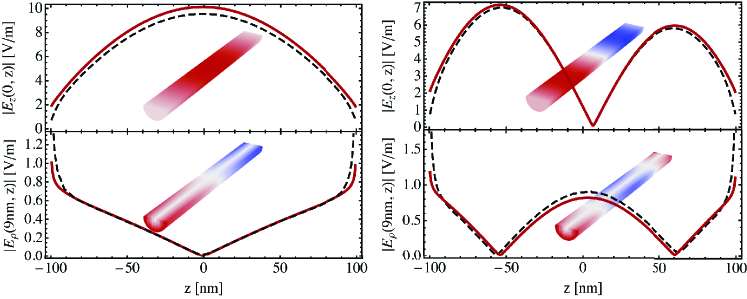
Figure 7: Induced electric field at the first (left) and second (right) resonance inside a gold nanowire with radius $a=10$ nm and length $l=200$ nm under slanting incidence ($\xi=\frac{\pi}{4},\,E_{0}^{\parallel}=1$). Each top panel show the $z$-components on the wire axis and the bottom panels the radial $\rho$-components 9 nm apart from the axis. The fields are obtained by HFSS (red solid line) and VC-IE (black dashed line).

To make sure that an appropriate space discretization $\Delta$ (slice thickness) is used when applying the VC-IE or SI-IE to realistic scattering problems, their convergence is studied. Figure 5 shows the dependence of the resonance frequencies on the space discretization $\Delta$ for a gold nanowire ($l=200\text{ nm},\,a=10\text{ nm}$) under slanting incidence ($\xi=\frac{\pi}{4}$). From the top to the bottom panel convergence of resonances of increasing order are shown. The calculations are performed with (i) the SI-IE solved by Hallen’s approach (dotted line), (ii) the regularized SI-IE (dashed line) and (iii) the VC-IE (solid line). It can be seen that (i) the converged result of the SI-IE does not depend on the way of solving it and (ii) a discretization of $\Delta=1$ nm already shows a deviation from the converged value of less than 1THz. Thus we choose a discretization of $\Delta=1$ nm in subsequent studies. In figure 6 the total scattering cross section as function of frequency for gold nanowires of different lengths but fixed radius, $a=10nm$, under normal incidence ($\xi=\frac{\pi}{2}$) are shown Kremers and Chigrin [2011]. The results of VC-IE, SI-IE and numerically rigorous DDA method are represented by solid, dashed and dotted lines, respectively. One can trace that (i) the deviation of both semi-analytical methods from the numerical exact DDA reference solution increase with decreasing aspect ratios of the wire and (ii) the accuracy of the VC-IE is slightly better than the one of the SI-IE. This behaviour was expected because the ansatz (47) for the internal field taken from the infinitely long wire becomes worse for decreasing aspect ratios. It is remarkable that for a wire with aspect ratio as low as $\frac{5}{2}$ ($l=50nm$) the relative deviation is less than 2%. But most important are the differences in execution time. The calculation of one frequency point in SI and VC integral equation method requires, respectively, about 1 and 2 seconds on one core of a modern workstation using Mathematica Wolfram . An additional advantage of the VC-IE despite its slightly better accuracy in the calculation of far field properties like the scattering cross section, is its ability to calculate even the near field of the plasmonic wire with high accuracy. To demonstrate this a comparison between the internal field obtained with the VC-IE and HFSS is shown in figure 7 for a gold nanowire ($l=200nm,\,a=10nm$) under slanting incidence ($\xi=\frac{\pi}{4}$). Here the radial component is calculated by assuming a solution of the form

$$\mathbf{E}(\rho,z)=\hat{\boldsymbol{\rho}}E_{\rho}(\rho,z)+\hat{\mathbf{z}}f(z)J_{0}\left(k_{\rho}\rho\right)$$ (53)

and enforcing the field to be divergence free. This results in

$$E_{\rho}(\rho,z)=-\frac{J_{1}(k_{\rho}\rho)}{k_{\rho}}\frac{\partial}{\partial z}f(z).$$ (54)

The left and right column of figure 7 show the field components for the first and second resonance of the wire respectively. The top panel on each column shows the $z$-component of the electric field at the wire axis and the bottom panel the $\rho$-component in $9nm$ distance from the axis. The $\rho$-component on the axis vanishes. The agreement between VC-IE and HFSS is very good. Thus we can conclude that using the calculated internal field in the form (53), the near field can be calculated with high accuracy by means of (25).

3 Plasmonic dimers

3.1 Two coupled nanoparticles

A considerable enhancment of electric field near a resonant plasmonic nanoparticle opens many application opportunities. Among others, one should mention strong interaction between the different type of emission centers and the nanoparticle, which results in strong modification of emission properties Kern and Martin [2011], Giannini et al. [2009], Kinkhabwala et al. [2009]. The field enhancement also allows to implement strong coupling among different nanoparticles themselves. A number of intriguing phenomena can be observed in coupled plasmonic structures, including Fano-type resonances Singh et al. [2011], Bachelier et al. [2008], Zhang et al. [2011], plasmon-induced transparency Zhang et al. [2008], Dong et al. [2010] (an analog of the electromagnetically induced transparency Harris [1997]) as well as unusual material properties of metamaterials Noginov et al. [2009], Bilotti et al. [2010].

To rigorously describe even the simplest type of the coupled nanoplasmonic system, i.e., two particles or a plasmonic dimer, one has to use direct numerical simulations Funston et al. [2009], Kern and Martin [2011]. Although a very intuitive coupled oscillator model Garrido Alzar et al. [2002] can explain the basic physical mechanisms of the particle plasmon interaction, it relies on phenomenological fitting parameters and is typically applicable only to the simplest case of parallel or anti-parallel particles. In this section we extend the coupled oscillator model to describe the coupling between two nanoparticles, which can be arbitrarily oriented with respect to one another. A sketch of the typical structure under consideration is shown in figure 3.

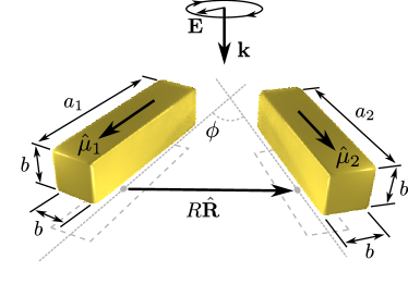
Figure 8: Sketch of the dimer structure under consideration. All relevant model parameters are indicated.

As was demonstrated in Sec. 2.1 the effect of the external field on a nanoparticle can always be described using an effective susceptibility tensor. Introducing particle polarizability tensor $\overleftrightarrow{\alpha}_{i}=\varepsilon_{0}\overleftrightarrow{\mathrm{X}}_{i}$ ($i=1,\,2$), the polarization (dipole moment) induced in one particle in presence of the second one can be written in the form

$$\tilde{\vec{\mu}}_{i}\left(\mathbf{r}_{i}\right)=\overleftrightarrow{\alpha}_{i}\mathbf{E}\left(\mathbf{r}_{i}\right)$$ (55)

with $\mathbf{E}\left(\mathbf{r}_{i}\right)$ being the total electric field at the particle $i$ position. Assuming further that electric dipole response of the particle can be modeled modeled as a response of the point dipole with the same polarizability the total field $\mathbf{E}\left(\mathbf{r}_{i}\right)$ can be expressed

$$\mathbf{E}\left(\mathbf{r}_{i}\right)=\overleftrightarrow{\alpha}_{i}\left(\mathbf{E}_{0}\left(\mathbf{r}_{i}\right)+\frac{k^{2}}{\varepsilon_{0}}\overleftrightarrow{\mathbf{G}}\left(\mathbf{R}\right)\tilde{\vec{\mu}}_{j}\right)$$ (56)

with $\mathbf{R}=\mathbf{r}_{j}-\mathbf{r}_{i}$, where $\mathbf{r}_{i}$ ($\mathbf{r}_{j}$) is a position of the $i$th ($j$th) particle. Here $\overleftrightarrow{\mathbf{G}}$ is the Green’s function determined from equation (23), and the second term is a contribution of the equivalent dipole of the second particle to the total field at the position of the first particle. To find an effective induced polarizability of the particles in the dimer, one has to solve the system (55) with the field expressed by (56). For example, substituting an expression of the induce dipole moment of the particle $j$ in the equation for the dipole moment of the particle $i$ we obtain

$$\tilde{\vec{\mu}}_{i}=\overleftrightarrow{\alpha}_{i}\mathbf{E}(\mathbf{r}_{i})=\\ \left(\overleftrightarrow{\alpha}_{i}+\frac{k^{2}}{\varepsilon_{0}}\overleftrightarrow{\alpha}_{i}\overleftrightarrow{\mathbf{G}}(\mathbf{R})\overleftrightarrow{\alpha}_{j}\right)\mathbf{E}_{0}+\\ \frac{k^{4}}{\varepsilon_{0}^{2}}\overleftrightarrow{\alpha}_{i}\overleftrightarrow{\mathbf{G}}(\mathbf{R})\overleftrightarrow{\alpha}_{j}\overleftrightarrow{\mathbf{G}}(-\mathbf{R})\tilde{\vec{\mu}}_{i}$$ (57)

which can be solved to obtain the unknown effective dipole moment $\tilde{\vec{\mu}}_{i}$

$$\tilde{\vec{\mu}}_{i}=\left[\overleftrightarrow{\mathbf{I}}-\frac{k^{4}}{\varepsilon_{0}^{2}}\overleftrightarrow{\alpha}_{i}\overleftrightarrow{\mathbf{G}}(\mathbf{R})\overleftrightarrow{\alpha}_{j}\overleftrightarrow{\mathbf{G}}(-\mathbf{R})\right]^{-1}\\ \left[\overleftrightarrow{\alpha}_{i}+\frac{k^{2}}{\varepsilon_{0}}\overleftrightarrow{\alpha}_{i}\overleftrightarrow{\mathbf{G}}(\mathbf{r})\overleftrightarrow{\alpha}_{j}\right]\mathbf{E}_{0}=\tilde{\overleftrightarrow{\alpha}}_{i}\mathbf{E}_{0}.$$ (58)

Here the effective polarizability $\tilde{\overleftrightarrow{\alpha}}_{i}$ of the particle $i$ in the presence of the particle $j$ has been introduced. Please note that this expression is valid in the point dipole approximation for an arbitrary mutial orientation of the nanoparticles.

A pair of electrical dipoles is general results in effective electric dipole, electric quadrupole, and magnetic dipole moments. The effective dipole moment $\vec{\mu}_{\mathrm{eff}}=\tilde{\vec{\mu}}_{1}+\tilde{\vec{\mu}}_{2}$ is given by a simple sum of the individual dipole moments $\tilde{\vec{\mu}}_{i}$ and results in an effective polarizability of the plasmonic dimer in the coupled dipole approximation given by

$$\overleftrightarrow{\alpha}_{\mathrm{eff}}=\sum_{i=1,2}\left[\overleftrightarrow{\mathbf{I}}-\frac{k^{4}}{\varepsilon_{0}^{2}}\overleftrightarrow{\alpha}_{i}\overleftrightarrow{\mathbf{G}}\overleftrightarrow{\alpha}_{j\neq i}\overleftrightarrow{\mathbf{G}}\right]^{-1}\\ \left[\overleftrightarrow{\alpha}_{i}+\overleftrightarrow{\alpha}_{i}\frac{k^{2}}{\varepsilon_{0}}\overleftrightarrow{\mathbf{G}}\overleftrightarrow{\alpha}_{j\neq i}\right].$$ (59)

The electric quadrupole and magnetic dipole moments are given respectively by

$$\overleftrightarrow{Q}=\left(\mathbf{r}_{1}\otimes\tilde{\vec{\mu}}_{1}+\tilde{\vec{\mu}}_{1}\otimes\mathbf{r}_{1}+\mathbf{r}_{2}\otimes\tilde{\vec{\mu}}_{2}+\tilde{\vec{\mu}}_{2}\otimes\mathbf{r}_{2}\right)$$ (60)

and

$$\mathbf{m}=-\frac{\mathrm{\mathrm{i}\omega}}{2}\left(\mathbf{r}_{1}\times\tilde{\vec{\mu}}_{1}+\mathbf{r}_{2}\times\tilde{\vec{\mu}}_{2}\right).$$ (61)

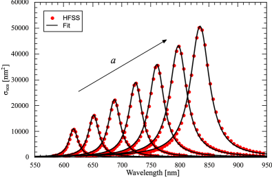
Figure 9: Scattering cross sections of single nanoblocks. Lengths are left to right from 60 nm to 120 nm with 10 nm step. Width and height of all nanoblocks are 20 nm.

Figure 10: Scattering cross section of the gold nanorods dimer for left circular polarized light calculated within coupled dipole model. Solid line is a result of contributions from all considered multipole terms. Dashed line is purely electric dipole contribution. Dotted line shows combined contribution of magnetic dipole and electric quadrupole. Gold rods are 100 nm apart and are rotated 45 degree with respect to each other. Rods are 80 nm and 75 nm long.

We further use developed couled dipole model to calculate a scattering cross section of the gold dimer. For small particles the dominant contribution to the first resonance is dipole in nature. Moreover if a particle is elongated, within the spectral range of the longitudinal plasmon-polariton resonance the contribution of the transverse resonances can be neglected. With a good approximation corresponding dipole polarizability can be described by the Lorentz model with all retardation effects included in the renormalized resonance frequency and damping (Sec. 2.3). In what follows we model both nanoparticles using dipole polarizability of the form

$$\overleftrightarrow{\alpha}_{j}=\frac{f_{j}\hat{\mu}_{j}\otimes\hat{\mu}_{j}}{\omega_{oj}^{2}-\omega^{2}-i\omega\gamma_{j}}\equiv\alpha_{j}\hat{\mu}_{j}\otimes\hat{\mu}_{j},$$ (62)

where the resonance frequency $\omega_{oj}$, damping constant $\gamma_{j}$ and amplitude $f_{j}$ are determined by the fit the corresponding numerical scattering cross section of the individual particles using the Lorentz model. In figure 9 scattering cross sections of the gold nanoblocks of different length are shown. Both finite element data (dots) and the results obtained using the fitting function (62) are presented, justifying the use of the proposed approach to modeling of the individual particles.

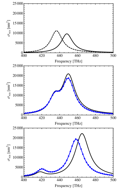
Figure 11: Scattering cross section of the gold nanorods dimer for different rod-to-rod distances. Left circular polarized light is considered. Distance between rods is 100 nm (middle panel) and 60 nm (bottom panel). Solid black lines are results of the coupled dipole model. Blue lines with dots are results of direct numerical simulations performed with finite element method (HFSS) Ansys . In the top panel scattering cross cross sections are shown for individual rods, 80 nm long (solid line) and 75 nm long (dashed line).

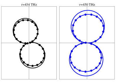
Figure 12: Far-field directionality diagrams are shown for two frequencies corresponding to two maxima in the scattering cross section. Directionality diagrams are shown in the dimer plane. Solid lines are results of the coupled dipole model. Lines with dots are results of direct numerical simulations performed with finite element method (HFSS) Ansys . Gold rods are 100 nm apart and are rotated 45 degrees with respect to each other. Rods are 80 nm and 75 nm long.

In figure 10 scattering cross section of the gold dimer build from 80 nm and 75 nm long nanoblocks is shown. Width and height of both nanoblocks is equal to 20 nm. Particles are situated 100 nm apart and at $45^{\circ}$ with respect to each other. Scattering cross section is calculated for the left-handed circular polarized light incident perpendicular to the dimer plane, taking into account only the electric dipole moment contributions (solid line), the electric quadrupole and magnetic dipole contributions (dotted line), and all available multipole contributions (dashed line) . One can clearly see that for the considered structure the electric dipole contribution is dominant and contributions from the higher order multipoles can be neglected.

In figures 11 and 12 comparison of the coupled dipole model (solid lines) with the direct numerical simulations using finite element method (lines with dots) is shown. In figure 11 scattering cross sections are shown for two distances between particles, namely 100 nm and 60 nm. One can clearly see that with decreasing the distance the quantitative agreement between analytical and numerical results becomes worse, but the qualitative agreement remains very reasonable. To appreciate the amount of the “cross-pushing” (repulsion) of the original resonances, the scattering cross sections of the individual nanblocks are presented in the top panel of figure 11. Proposed coupled dipole model demonstrate very good accuracy at moderate particle separations both for integral and differential scattering properties as can be seen from figure 12, where a comparison of the analytical and numerical far-field directionality diagrams is shown.

3.2 Planar chiral meta-atoms

Having established that coupled dipole approximation is valis at least in the case of planar arrangements of nanoblocks in the dimer, we proceed to derive the effective material parameters.

We begin by rewriting the equation (59), using (62), in the form

$$\overleftrightarrow{\alpha}_{\text{eff}}= \frac{1}{1-\alpha_{1}\alpha_{2}\kappa^{2}}\cdot\biggl{[}\alpha_{1}\hat{\mu}_{1}\otimes\hat{\mu}_{1}+\alpha_{2}\hat{\mu}_{2}\otimes\hat{\mu}_{2}$$

$$+\alpha_{1}\alpha_{2}\kappa\left(\hat{\mu}_{1}\otimes\hat{\mu}_{2}+\hat{\mu}_{2}\otimes\hat{\mu}_{1}\right)\biggr{]}$$

$$\equiv \alpha_{1}^{\text{eff}}\hat{\mu}_{1}\otimes\hat{\mu}_{1}+\alpha_{2}^{\text{eff}}\hat{\mu}_{2}\otimes\hat{\mu}_{2}$$

$$+\alpha_{3}^{\text{eff}}\left(\hat{\mu}_{1}\otimes\hat{\mu}_{2}+\hat{\mu}_{2}\otimes\hat{\mu}_{1}\right).$$ (63)

where the unit vectors $\hat{\mu}_{j}$ denote the orientation of the rods (see figure 8), and$\kappa$ defines the coupling coefficient between the rods:

$$\kappa=\frac{k^{2}}{\varepsilon_{0}}\left[G_{I}\left(\hat{\mu}_{1}\cdot\hat{\mu}_{2}\right)+G_{R}\left(\hat{\mu}_{1}\cdot\hat{\mathbf{R}}\right)\left(\hat{\mu}_{2}\cdot\hat{\mathbf{R}}\right)\right].$$ (64)

The effective permittivity tensor $\overleftrightarrow{\varepsilon}_{\text{eff}}$ is derived from $\overleftrightarrow{\alpha}_{\text{eff}}$ in equation. (63) as

$$\overleftrightarrow{\varepsilon}_{\text{eff}}=\overleftrightarrow{\mathrm{I}}-(\varepsilon_{0}V_{\text{cell}})^{-1}\overleftrightarrow{\alpha}_{\text{eff}}.$$ (65)

In axial representation, $\overleftrightarrow{\varepsilon}_{\text{eff}}$ can be expressed as

$$\overleftrightarrow{\varepsilon}_{\text{eff}}=\overleftrightarrow{\mathrm{I}}+[\alpha_{1}^{\mathrm{eff}}/(2\epsilon_{0}V_{\mathrm{cell}})]\left(\mathbf{c}_{+}\otimes\mathbf{c}_{-}+\mathbf{c}_{-}\otimes\mathbf{c}_{+}\right)$$ (66)

where the complex vectors $\mathbf{c}_{\pm}=\left(\hat{\mu}_{1}+\eta_{\pm}\hat{\mu}_{2}\right)$ determine the directions of the optical axes, and $\eta_{\pm}$ are given by

$$\eta_{\pm}=\frac{\alpha_{3}^{\mathrm{eff}}\pm\sqrt{\left(\alpha_{3}^{\mathrm{eff}}\right)^{2}-\alpha_{1}^{\mathrm{eff}}\alpha_{2}^{\mathrm{eff}}}}{\alpha_{1}^{\mathrm{eff}}}.$$ (67)

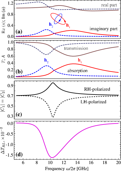
Figure 13: (Color online) (a) Refractive indices for two co-rotating elliptically polarized eigenwaves $\mathbf{h}_{1,2}$ of $\overleftrightarrow{N}_{H}$ in equation (68). (b) Transmission and absorption for incident wave with polarization given by $\mathbf{h}_{1,2}$. (c) Absolute value of the complex projection coefficients $C_{1,2}$ [see equation (69)] for RH (solid) and LH (dashed) circularly polarized incident wave. (d) Analytically calculated difference in transmission for LH/RH-polarized incident wave. Here $a_{1}=13$ mm, $a_{2}=10$ mm, $d=10$ mm, $\phi=45^{\circ}$, and $\psi=0^{\circ}$

The dielectric permittivity tensor (66) corresponds to an absorbing nonmagnetic crystal, which in general has two distinct eigenmodes with different polarizations, phase velocities, and absorption coefficients. These eigenmodes $\mathbf{h}_{1,2}$ and their associated refractive indices $n_{1,2}$ are given by eigenvectors and eigenvalues of the refractive index tensor Barkovsky [1976]

$$\overleftrightarrow{N}_{H}=\left[\left(-\mathbf{n}^{\times}\overleftrightarrow{\varepsilon}_{\text{eff}}^{-1}\mathbf{n}^{\times}\right)^{-}\right]^{1/2}.$$ (68)

Here $\mathbf{n}$ is a unit vector of the wave normal. The operator $\mathbf{n}^{\times}$ acts on a vector $\mathbf{u}$ in such a way that the result is the vector cross product: $(\mathbf{n}^{\times})\mathbf{u}=\left[\mathbf{n}\times\mathbf{u}\right]$. The tensor $\overleftrightarrow{A}^{-}$ is defined as a pseudoinverse to $\overleftrightarrow{A}$ ($\overleftrightarrow{A}^{-}\overleftrightarrow{A}=\overleftrightarrow{\mathrm{I}}-\mathbf{n}\otimes\mathbf{n}$) and is introduced in place of the true inverse tensor ($\overleftrightarrow{A}^{-1}$), which does not exist for tensors with zero determinant such as $\mathbf{n}^{\times}$.

In figure 13a, the real and imaginary parts of the refractive indices for the two eigenmodes ($n_{1,2}$) are shown for propagation direction orthogonal to the meta-atoms plane. One can clearly see that the absorption bands for the two eigenmodes are different. This is characteristic for dichroic media, and it was shown earlier that circular or elliptical dichroism is attributable to the optical manifestations of planar chirality Zhukovsky et al. [2009]. The eigenvectors $\mathbf{h}_{1,2}$ turn out to correspond to co-rotating elliptical polarizations with orthogonal principal axes (see inset in figure 13), which is a signature crystallographic property of planar metamaterials Fedotov et al. [2006], Plum et al. [2009].

Based on the effective permittivity$\overleftrightarrow{\varepsilon}_{\text{eff}}$, one can determine the optical spectra using the generalized transfer matrix approach (see, e.g., Borzdov [1997]). Figure 13b shows the transmission and absorption spectra of the medium given by (66) for an incident wave with polarization coincident with the eigenmodes ($\mathbf{h}_{1,2}$). The dips in the transmission spectra can be seen, in clear correspondence with the absorption bands. Due to the small variation in the real part of the refractive indices, reflection from such an effective medium slab is fairly small and does not contribute to the transmission dips.

For an arbitrarily polarized incident wave, the effective medium acts as an absorbing polarizing (dichroic) filter splitting the incident field $\mathbf{H}$ into two waves with polarizations parallel to the crystal eigenvectors $\mathbf{h}_{1,2}$ as

$$\mathbf{H}=C_{1}\mathbf{h}_{1}+C_{2}\mathbf{h}_{2}$$ (69)

where $C_{1,2}$ are complex projection coefficients. The transmission of the effective medium is then determined, on the one hand, by the relations between $C_{1,2}$, and on the other hand, on the relations between the absorption coefficients for the eigenwaves.

Figure 13c shows the projection coefficients $C_{1,2}$ for circularly polarized incident waves. In this case, it can be seen that $|C_{1}|=|C_{2}|$. However, in the spectral range of strong absorption the coupling of RH and LH incident waves to the crystal eigenmodes $\mathbf{h}_{1,2}$ is very different ($C_{1,2}^{R}\neq C_{1,2}^{L}$). Hence, circularly polarized waves with different handedness interact with the metamaterial with a different strength, and consequently, have different transmittance ($T_{R}\neq T_{L}$). For planar geometry, reversing the handedness of the incident wave polarization is equivalent to reversing the direction of incidence or exchange the structure with its enantiomeric counterpart (see figure (1)b,d). Hence, enantiomeric asymmetry in the transmission $\Delta T_{RL}=T_{R}-T_{L}$ (figure 13d) can be used to quantify the “strength” of planar chiral properties in a particular structure. It can be seen that the maximum value of $\Delta T_{RL}$ corresponds to the overlap between the different absorption bands in the dimer.

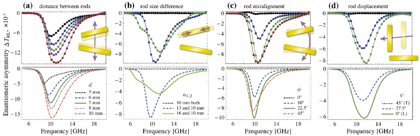
Figure 14: (Color online) Numerical (top) and analytical (bottom) dependence of $\Delta T_{RL}$ on (a) inter-rod distance $d$, (b) difference in rod length $a_{1}-a_{2}$, (c) rod misalignment angle $\phi$ as in figure 8, and (c) rod displacement angle $\psi$ for $\phi=90^{\circ}$ (as the dimer changes between T- and L-shaped). Unless specified otherwise, $a_{1}=13$ mm, $a_{2}=10$ mm, $d=6$ mm, $\phi=45^{\circ}$, and $\psi=0^{\circ}$.

Figure 14 shows the spectra $\Delta T_{RL}(\omega)$ for various shapes of the dimer, analytical results from the equations (62)–(63) compared to the results of direct 3D frequency-domain numerical simulations Ansys . It can be seen that the effective medium model offers a good coincidence with numerical results.

When the dimer has an in-plane mirror symmetry, the 2D enantiomers become indistinguishable and such a structure must necessarily be achiral ($\Delta T_{RL}=0$). For the geometrical transformation considered, an in-plane mirror symmetry is achieved in the following cases: (i) for rods of equal length (V-shaped dimer, figure 14b); (ii) for parallel rods (II-shaped dimer, figure 14c); (iii) for a T-shaped dimer (figure 14d). In all these cases, the analytical model correctly predicts the absence of enantiomeric asymmetry.

Otherwise, the dimers are seen to exhibit chiral properties, which are stronger when enantiomers are more distinct geometrically. So there is an optimum rod misalignment angle $\phi\simeq 22.5^{\circ}$ in figure 14c. It is also necessary that the absorption resonances corresponding to individual eigenpolarizations (figure 13c), and hence the resonances of the individual rods, have some degree of spectral overlap. Hence, $\Delta T_{RL}$ depends on the length mismatch between the rods in a non-monotonic way: it first increases when the dimer deviates from the achiral V-shape, reaches a maximum value, and then decreases again with a pronounced resonance splitting as $\Delta a$ becomes greater (see figure 14b).

It can also be noticed that $\Delta T_{RL}$ becomes smaller as the distance between the rods decreases (figure 14a). This can be explained by cross-pushing of the absorption resonances due to an increase in the inter-rod coupling for smaller inter-rod distances. The evidence of such cross-pushing can be inferred from figure 11.

If the rods were arranged in a non-planar fashion (e.g., as shown in figure 1c), the magnetic dipole and electric quadrupole contribution [equations (60) and (61)] would be expected to contribute to the dimer’s electromagnetical response much more significantly. It can be shown (the detailed calculation will be available in a forthcoming report) that 3D chiral properties and giant optical activity effects Kuwata-Gonokami et al. [2005] can be expected from such dimers. This is fully supported by the observation that some non-planar dimers are geometrically similat to known 3D chiral meta-atoms (see figures 1a,c).

Note, finally, that we have been considering an isolated plasmonic meta-atom throughout the paper, while real metamaterials contain a multitude of meta-atoms. Hence, the results obtained here are directly applicable to metamaterials in the approximation that the meta-atoms are sufficiently sparse and do not interact with each other. Importantly, this also means that chiral properties in the metamaterials under study are intrinsic (attributable to the geometry of the meta-atom itself) rather than extrinsic (attributable to the meta-atom arrangement, as in tilted-cross arrays Volkov et al. [2009]). This agrees with earlier time-domain simulation results Kremers et al. [2009]. With the proposed model extended to include the inter-atom coupling (see, e.g., Novitsky et al. [2010]), explicit account of intrinsic vs. extrinsic effects in 2D and 3D chiral metamaterials can be given. Combining the intrinsic and extrinsic contribution in the same metamaterial can be used to maximize its chiral properties.

4 Conclusion

We have systematically described the basic physics of light interaction with plasmonic nanoparticles. Starting with the general expression for the polarizability of one metallic particle (a plasmonic monomer) in an external electromagnetic field, we have explored several ways to simplify it for the approximation of the nanoparticle size being much smaller than the wavelength (the Rayleigh approximation). We have also investigated the corrections to the Rayleigh approach by accounting for the retardation effects. We have introduced accurate and numerically efficient 1D semi-analytical method to solve the problem of light scattering on metallic nanowires for optical frequency range. We have discussed the applicability of the method and its accuracy in comparison with the direct numerical simulations. Applications of these results to plasmonic nanoantennas are outlined.

We have also applied a coupled dipole approach to a pair of closely located rod-like nanoparticles (a plasmonic dimer). By accounting for the interaction between the partices in the dimer, we have arrived at analytic expressions of the dimer’s polarizability. The effective macroscopic material parameters have then been calculated. These parameters are attributable to an effective medium corresponding to a sparse arrangement of nanoparticles, i.e., a metamaterial where plasmonic dimers have the function of “meta-atoms”. It is shown that planar dimers consisting of rod-like particles generally possess elliptical dichroism Zhukovsky et al. [2009] and function as atoms for planar chiral metamaterialsFedotov et al. [2006], Plum et al. [2009]. It is worth noting that we have been able to design “meta-atom” structure possessing the previously reported polarization effects, while being considerably simpler with respect to analysis and fabrication. Indeed, it is far easier to fabricate an array of nanorods than it is to fabricate an array of more complicated objects such as nanogammadions, and the difference becomes more pronounced as the length scales go down. Hence, the results of this work can form theoretical grounds to new, cheaper, easier-to-make chiral metamaterials in the optical domain.

The authors wish to acknowledge financial support from the Deutsche Forschungsgemeinschaft (DFG) Research Unit FOR 557.

References

- Mackay and Lakhtakia [2009] T. Mackay and A. Lakhtakia. Negative refraction, negative phase velocity, and counterposition in bianisotropic materials and metamaterials. Physical Review B, 79(23), 2009.
- McCall [2008] M. McCall. A covariant theory of negative phase velocity propagation. Metamaterials, 2(2-3), 2008.
- Noginov et al. [2009] M. A. Noginov, Yu. A. Barnakov, G. Zhu, T. Tumkur, H. Li, and E. E. Narimanov. Bulk photonic metamaterial with hyperbolic dispersion. Appl. Phys. Lett., 94(15), 2009.
- Schurig et al. [2006] D. Schurig, J. J. Mock, B. J. Justice, S. A. Cummer, J. B. Pendry, A. F. Starr, and D. R. Smith. Metamaterial electromagnetic cloak at microwave frequencies. Science (New York, N.Y.), 314(5801), 2006.
- Cai et al. [2007] Wenshan Cai, Uday K. Chettiar, Alexander V. Kildishev, and Vladimir M. Shalaev. Optical cloaking with metamaterials. Nature Photonics, 1(4), 2007.
- Bilotti et al. [2010] F. Bilotti, S. Tricarico, and L. Vegni. Plasmonic Metamaterial Cloaking at Optical Frequencies. IEEE Transactions on Nanotechnology, 9(1), 2010.
- Leonhardt [2011] U. Leonhardt. To invisibility and beyond. Nature, 471(7338), 2011.
- Narimanov and Kildishev [2009] Evgenii E. Narimanov and Alexander V. Kildishev. Optical black hole: Broadband omnidirectional light absorber. Appl. Phys. Lett., 95(4), 2009.
- Shalaev [2008] Vladimir M. Shalaev. Transforming light. Science, 322(5900), 2008.
- Kuwata-Gonokami et al. [2005] M. Kuwata-Gonokami, N. Saito, Y. Ino, M. Kauranen, K. Jefimovs, T. Vallius, J. Turunen, and Y. Svirko. Giant optical activity in quasi-two-dimensional planar nanostructures. Physical Review Letters, 95, 2005.
- Potts et al. [2004] A. Potts, A. Papakostasa, D. M. Bagnalla, and N. I. Zheludev. Planar chiral meta-materials for optical applications. Microelectronic Engineering, 73-74(1), 2004.
- Fedotov et al. [2006] V. A. Fedotov, P. L. Mladyonov, S. L. Prosvirnin, A. V. Rogacheva, Y. Chen, and N. I. Zheludev. Asymmetric propagation of electromagnetic waves through a planar chiral structure. Physical Review Letters, 97, 2006.
- Plum et al. [2009] E. Plum, V. A. Fedotov, and N. I. Zheludev. Planar metamaterial with transmission and reflection that depend on the direction of incidence. Applied Physics Letters, 94, 2009.
- Zhukovsky et al. [2009] S. V. Zhukovsky, V. M. Galynsky, and A. V. Novitsky. Elliptical dichroism: operating principle of planar chiral metamaterials. Optics Letters, 34(13), 2009.
- Simovski et al. [2002] C. R. Simovski, E. Verney, S. Zouhdi, and A. Fourrier-Lamer. Homogenization of planar bianisotropic arrays on the dielectric interface. Electromagnetics, 22, 2002.
- Smith et al. [2002] D. Smith, S. Schultz, P. Markoš, and C. Soukoulis. Determination of effective permittivity and permeability of metamaterials from reflection and transmission coefficients. Physical Review B, 65(19), 2002.
- Smith and Pendry [2006] D. R. Smith and J. B. B. Pendry. Homogenization of metamaterials by field averaging. Journal of the Optical Society of America B, 23(3), 2006.
- Baena et al. [2008] J. D. Baena, L. Jelinek, R. Marques, and M. Silveirinha. Unified homogenization theory for magnetoinductive and electromagnetic waves in split ring metamaterial. Physical Review A, 78, 2008.
- Myroshnychenko et al. [2008a] Viktor Myroshnychenko, Jessica Rodríguez-Fernández, Isabel Pastoriza-Santos, Alison M. Funston, Carolina Novo, Paul Mulvaney, Luis M. Liz-Marzán, and F. Javier García de Abajo. Modelling the optical response of gold nanoparticles. Chem. Soc. Rev., 37, 2008a.
- Romero [2009] F. J. Romero, I.and García De Abajo. Anisotropy and particle-size effects in nanostructured plasmonic metamaterials. Optics Express, 17(24), 2009.
- Balanis [1989] C. A. Balanis. Advanced engineering electromagnetics. Wiley, 1989.
- Volakis [2007] J. Volakis. Antenna Engineering Handbook, Fourth Edition. McGraw-Hill Professional, 2007.
- Bharadwaj et al. [2009] P. Bharadwaj, B. Deutsch, and L. Novotny. Optical Antennas. Advances in Optics and Photonics, 1(3), 2009.
- Mühlschlegel et al. [2005] P. Mühlschlegel, H. J. Eisler, O. J. F. Martin, B. Hecht, and D. W. Pohl. Resonant optical antennas. Science, 308(5728), 2005.
- Rogobete et al. [2007] L. Rogobete, F. Kaminski, M. Agio, and V. Sandoghdar. Design of plasmonic nanoantennae for enhancing spontaneous emission. Optics Letters, 32(12), 2007.
- Taminiau et al. [2008] T. H. Taminiau, F. D. Stefani, F. B. Segerink, and N. F. van Hulst. Optical antennas direct single-molecule emission. Nature Photonics, 2(4), 2008.
- Raschke et al. [2003] G. Raschke, S Kowarik, T. Franzl, C. Sönnichsen, T. A. Klar, J. Feldmann, A Nichtl, and K. Kürzinger. Biomolecular Recognition Based on Single Gold Nanoparticle Light Scattering. Nano Letters, 3(7), 2003.
- Atwater and Polman [2010] H. A. Atwater and A. Polman. Plasmonics for improved photovoltaic devices. Nature materials, 9(3), 2010.
- Bladel [2007] J. Bladel. Electromagnetic fields. Wiley-IEEE, 2007.
- Bozhevolnyi and Lozovski [2000] Sergey I. Bozhevolnyi and Valeri Z. Lozovski. Self-consistent model for second-harmonic near-field microscopy. Phys. Rev. B, 61(16), 2000.
- Bozhevolnyi et al. [2001] S. Bozhevolnyi, V. Lozovski, and Yu. Nazarok. Diagram method for exact solution of the problem of scanning near-field microscopy. Optics and Spectroscopy, 90(3):416–425, 2001.
- Sheng [2006] P. Sheng. Introduction To Wave Scattering, Localization And Mesoscopic Phenomena. Springer-Verlag, 2006.
- Keller et al. [1993] Ole Keller, Mufei Xiao, and Sergey Bozhevolnyi. Configurational resonances in optical near-field microscopy: a rigorous point-dipole approach. Surface Science, 280(1-2), 1993.
- Abrikosov A. A. [1965] Dzyaloshinskii L. Ye. Abrikosov A. A., Gorkov L. P. Quantum Field Theoretical Methods in Statistical Physics. Oxford: Pergamon, 1965.
- Lee et al. [1980] S. W. Lee, J. Boersma, C. L. Law, and G. Deschamps. Singularity in Green’s function and its numerical evaluation. Antennas and Propagation, IEEE Transactions on, 28(3), 1980.
- Yaghjian [1980] A.D. Yaghjian. Electric dyadic Green’s functions in the source region. Proceedings of the IEEE, 68(2), 1980.
- Karam [1997] M. A. Karam. Electromagnetic wave interactions with dielectric particles. I. Integral equation reformation. Applied Optics, 36(21), 1997.
- Myroshnychenko et al. [2008b] V. Myroshnychenko, J. Rodríguez-Fernández, I. Pastoriza-Santos, A. M. Funston, C. Novo, P. Mulvaney, L. M. Liz-Marzán, and F. J. García De Abajo. Modelling the optical response of gold nanoparticles. Chemical Society reviews, 37(9), 2008b.
- Yurkin and Hoekstra [2007] M. Yurkin and A. Hoekstra. The discrete dipole approximation: An overview and recent developments. Journal of Quantitative Spectroscopy and Radiative Transfer, 106(1-3), 2007.
- Myroshnychenko et al. [2008c] V. Myroshnychenko, E. Carbó-Argibay, I. Pastoriza-Santos, J. Pérez-Juste, L. M. Liz-Marzán, and F. J. García de Abajo. Modeling the Optical Response of Highly Faceted Metal Nanoparticles with a Fully 3D Boundary Element Method. Advanced Materials, 20(22), 2008c.
- Jin [2002] J. M. Jin. The Finite Element Method in Electromagnetics. Wiley-IEEE Press, 2002.
- Stannigel et al. [2009] K. Stannigel, M. König, J. Niegemann, and K. Busch. Discontinuous Galerkin time-domain computations of metallic nanostructures. Optics Express, 17(17), 2009.
- Hesthaven [2002] J Hesthaven. Nodal High-Order Methods on Unstructured Grids I. Time-Domain Solution of Maxwell’s Equations. Journal of Computational Physics, 181(1), 2002.
- Taflove and Hagnes [2000] A. Taflove and S. C. Hagnes. Computational Electrodynamics: The Finite-Difference Time-Domain Method. Artech House, 2000.
- Yurkin et al. [2007] M. Yurkin, V. Maltsev, and A. Hoekstra. The discrete dipole approximation for simulation of light scattering by particles much larger than the wavelength. Journal of Quantitative Spectroscopy and Radiative Transfer, 106(1-3), 2007.
- [46] Ansys. Hfss. http://www.ansoft.com/products/hf/hfss/.
- Kremers and Chigrin [2011] C. Kremers and D.N. Chigrin. Light scattering on nanowire antennas: A semi-analytical approach. Photonics and Nanostructures - Fundamentals and Applications, DOI 10.1016/j.photonics.2011.03.004, 2011.
- Orfanidis [2010] S. J. Orfanidis. Electromagnetic Waves and Antennas. http://www.ece.rutgers.edu/~orfanidi/ewa/, 2010.
- Bohren and Huffman [1998] C. F. Bohren and D. R. Huffman. Absorption and Scattering of Light by Small Particles (Wiley science paperback series). Wiley-VCH, 1998.
- Hanson [2006] G. W. Hanson. On the Applicability of the Surface Impedance Integral Equation for Optical and Near Infrared Copper Dipole Antennas. IEEE Transactions on Antennas and Propagation, 54(12), 2006.
- [51] Wolfram. Mathematica 8. http://www.wolfram.com/mathematica.
- Kern and Martin [2011] A. M. Kern and O. J. F. Martin. Excitation and Reemission of Molecules near Realistic Plasmonic Nanostructures. Nano letters, 11(2), 2011.
- Giannini et al. [2009] V. Giannini, J. A. Sánchez-Gil, O. L. Muskens, and J. G. Rivas. Electrodynamic calculations of spontaneous emission coupled to metal nanostructures of arbitrary shape: nanoantenna-enhanced fluorescence. Journal of the Optical Society of America B, 26(8), 2009.
- Kinkhabwala et al. [2009] A. Kinkhabwala, Z. Yu, S. Fan, Y. Avlasevich, K. Müllen, and W. E. Moerner. Large single-molecule fluorescence enhancements produced by a bowtie nanoantenna. Nature Photonics, 3(11), 2009.
- Singh et al. [2011] R. Singh, I. A. I. Al-Naib, M. Koch, and W. Zhang. Sharp Fano resonances in THz metamaterials. Optics Express, 19(7), 2011.
- Bachelier et al. [2008] G. Bachelier, I. Russier-Antoine, E. Benichou, C. Jonin, N. Del Fatti, F. Vallée, and P.-F. Brevet. Fano Profiles Induced by Near-Field Coupling in Heterogeneous Dimers of Gold and Silver Nanoparticles. Physical Review Letters, 101(19), 2008.
- Zhang et al. [2011] S. Zhang, K. Bao, N. J. Halas, H. Xu, and P. Nordlander. Substrate-Induced Fano Resonances of a Plasmonic Nanocube: A Route to Increased-Sensitivity Localized Surface Plasmon Resonance Sensors Revealed. Nano Letters, 11(4), 2011.
- Zhang et al. [2008] S. Zhang, D. Genov, Y. Wang, M. Liu, and X. Zhang. Plasmon-Induced Transparency in Metamaterials. Physical Review Letters, 101(4), 2008.
- Dong et al. [2010] Z. G. Dong, H. Liu, M. X. Xu, T. Li, S. M. Wang, S. N. Zhu, and X. Zhang. Plasmonically induced transparent magnetic resonance in a metallic metamaterial composed of asymmetric double bars. Optics Express, 18(17), 2010.
- Harris [1997] S. E. Harris. Electromagnetically induced transparency. Physics Today, 50(7), 1997.
- Funston et al. [2009] A. M. Funston, C. Novo, T. J. Davis, and P. Mulvaney. Plasmon coupling of gold nanorods at short distances and in different geometries. Nano letters, 9(4), 2009.
- Garrido Alzar et al. [2002] C. L. Garrido Alzar, M. A. G. Martinez, and P. Nussenzveig. Classical analog of electromagnetically induced transparency. American Journal of Physics, 70(1), 2002.
- Barkovsky [1976] L. M. Barkovsky. On the refractive index tensor in crystallooptics. Sov. Phys. Crystallogr., 21, 1976.
- Borzdov [1997] G. N. Borzdov. Frequency domain wave splitting techniques for plane stratified bianisotropic media. Journal of Mathematical Physics, 38, 1997.
- Volkov et al. [2009] S. N. Volkov, K. Dolgaleva, R. W. Boyd, K. Jefimovs, J. Turunen, Y. Svirko, B. K. Canfield, and M. Kauranen. Optical activity in diffraction from a planar array of achiral nanoparticles. Physical Review A, 79, 2009.
- Kremers et al. [2009] Christian Kremers, Sergei V. Zhukovsky, and Dmitry N. Chigrin. Numerical time-domain simulations of planar chiral metamaterials. In Dmitry N. Chigrin, editor, Theoretical and Computational Nanophotonics: Proceedings of the 2nd International Workshop, volume 1176 of AIP Conference Proc., 2009.
- Novitsky et al. [2010] A. V. Novitsky, V. M. Galynsky, and Sergei V. Zhukovsky. Asymmetric transmission in planar chiral split-ring metamaterials: Microscopic Lorentz-theory approach. http://arxiv.org/abs/1012.5119, 2010.