An Exact Formula for the Statistics of the Current in the TASEP with Open Boundaries

Abstract

We study the totally asymmetric exclusion process (TASEP) on a finite one-dimensional lattice with open boundaries, i.e., in contact with two reservoirs at different potentials. The total (time-integrated) current through the system is a random variable that scales linearly with time in the long time limit. We give a parametric representation for the generating function of the cumulants of the current, which is related to the large deviation function by Laplace transform. This formula is valid for all system sizes and for all values of the boundary coupling parameters.

I Introduction

The asymmetric simple exclusion process (ASEP) is one of the fundamental models in non-equilibrium statistical mechanics. The ASEP involves particles that perform asymmetric jumps on a discrete lattice under the exclusion constraint: two particles cannot occupy the same site at the same time. This very simple and minimal system appears as a building block in more realistic descriptions for low-dimensional transport with constraints. Such phenomena occur in various contexts and scales ranging from micrometric cellular motors to traffic networks PaulK ; Zia . The remarkable properties of the ASEP and its numerous variants have stimulated hundreds of studies during the last two decades. The ramifications of this mundane-looking model through non-equilibrium statistical mechanics, combinatorics, probability, random matrices and representation theory are tremendous MartinReview ; DerridaRep ; FerrariPatrick ; PaulK ; Sasamoto ; Schutz ; Spohn .

Generically, a system out of equilibrium carries at least one non-vanishing current in its steady state (this is related to the breaking of detailed balance). Such currents can be considered as archetypal observables for non-equilibrium behaviour Zia . Classifying the different independent stationary currents in a given system, identifying some generic features and relations obeyed by the distributions of these currents and calculating their statistical properties as functions of the control parameters, are some of the important tasks in non-equilibrium statistical physics. Current fluctuations are usually non-Gaussian: their characteristics can be quantified by the moments of the current (mean-value, variance, skewness, kurtosis…) or by a large-deviation function that measures the probability for the current to assume a non-typical value. There is growing evidence that large-deviation functions play a crucial role in non-equilibrium statistical physics, akin to that of thermodynamic potentials at equilibrium DerrReview ; Touchette .

Currents transport information from one part of the system to another. In particular, in a system far from equilibrium, boundary conditions can drastically alter the behaviour of the bulk even if interactions are short-ranged (in contrast with the generic case at equilibrium). For example, as was recognized in the earliest studies Krug ; Janowski , phase-transitions can be induced by the boundaries or by a localized alteration of the dynamical rules. It is therefore crucial to specify the boundary conditions (e.g. periodic, twisted, open boundaries, infinite system…). The phenomenology of the system and the mathematical techniques that are used to analyse it depend strongly on the chosen boundary conditions.

In the present work we consider the exclusion process on a finite lattice with open boundaries, which can be viewed as a model for a conducting rod in contact with two reservoirs that are not in thermodynamic equilibrium with each other (for example, they are at different temperatures, or have different chemical, mechanical or electrical potentials). Besides, an external field may be applied to the system. This external field and the reservoirs drive a current through the system and, in the long time limit, the connecting rod reaches a non-equilibrium stationary state. Our aim is to study the statistics of this stationary current. We give explicit formulae, equations (15) to (19), for the cumulant generating function of the totally asymmetric exclusion process (TASEP) with open boundaries that are valid for arbitrary values of the entrance and exit rates and for all values of the system size $L$. We emphasize the fact that our results are of combinatorial nature and not only asymptotic: they describe the TASEP in all possible regimes, including the phase-transition lines. This is in contrast with the asymptotic expression for the large-deviation function of the current obtained very recently using the Bethe Ansatz deGierNew . Indeed, as of today, the Bethe Ansatz for the open TASEP deGier1 seems to be tractable only in the $L\to\infty$ limit, and only inside the low and high density phases far from the phase-transition lines. We show that the formula obtained in deGierNew for $L\to\infty$ can be retrieved as a limiting case of our general results. The parametric representation we have found is obtained by using the Matrix Ansatz technique DEHP ; MartinReview . The calculations are very cumbersome and some combinatorial patterns have been guessed rather than fully calculated. The formulae we obtain must therefore be considered as conjectures. But as we shall explain, the results are exact albeit they have been obtained, at present, in a non-rigorous manner. They have also been thoroughly verified against exact computations for systems of small sizes. Besides, all known special cases can be deduced from our general result.

The outline of this work is as follows. In section II, we recall the definition of the model and the basic properties that will be used later (the master equation, the matrix solution and the phase diagram). Section III contains the main results of this work; we first restate the problem of current fluctuations in the standard mathematical framework, and then describe the simpler case where all the parameters in the system are equal and taken to be 1. The general formulae are presented in III.3 and are followed by a physical discussion of the behaviour of the system through the phase diagram; we also discuss some connections with previously known results. In section IV, we explain the line of reasoning that we have followed to obtain the formula for the current fluctuation, show where the unproven assumptions reside, and describe some numerical verifications. The last section is devoted to concluding remarks. A detailed derivation of the large $L$ limit deGierNew from the general formula is given in the appendix.

II Definition of the TASEP and basic properties

We consider the totally asymmetric simple exclusion process (TASEP) on a finite lattice of size $L$ with open boundaries. Each site of the system can be occupied by at most one particle (exclusion condition). The dynamics of the model is defined by the following stochastic rules (see figure 1): a particle at a site $i$ in the bulk of the system (with $1\leq i\leq L-1$) can jump with rate $p=1$ (i.e with probability $dt$ during the time interval $dt$) to the site $i+1$ if this target site is vacant; if site 1 is empty, a particle can enter with rate $\alpha$; a particle at site $L$ can leave the system with rate $\beta$. The entrance and exit rates represent the coupling of the finite system with infinite reservoirs located at its boundaries. At a given time, the system is in one of its $2^{L}$ possible configurations and evolves according to its stochastic dynamics as a Markov process. The evolution of the system can be encoded in the Markov matrix $M$ as follows: the probability $P_{t}({\mathcal{C}})$ of being in configuration ${\mathcal{C}}$ at time $t$ satisfies the master equation

$$\frac{dP_{t}({\mathcal{C}})}{dt}=\sum_{{\mathcal{C}^{\prime}}}M({\mathcal{C}},{\mathcal{C}^{\prime}})P_{t}({\mathcal{C}^{\prime}})\,.$$ (1)

The non-diagonal matrix element $M({\mathcal{C}},{\mathcal{C}^{\prime}})$ represents the transition rate from ${\mathcal{C}^{\prime}}$ to ${\mathcal{C}}$. The diagonal part $M({\mathcal{C}},{\mathcal{C}})=-\sum_{{\mathcal{C}^{\prime}}\neq{\mathcal{C}}}M({\mathcal{C}^{\prime}},{\mathcal{C}})$ represents (minus) the exit rate from ${\mathcal{C}}$. The Markov matrix is a stochastic matrix: the sum of the elements in any given column vanishes.

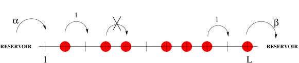
Figure 1: Illustration of the TASEP with open boundaries on a finite lattice with $L$ sites.

In the long time limit, the system reaches a steady state in which each of the $2^{L}$ possible configurations occurs with a stationary probability. This steady state probability lies in the kernel of the Markov Matrix: the rules of the ASEP ensure that this kernel is non-degenerate and that all other eigenvalues of $M$ have strictly negative real-parts that correspond to relaxation states with a possible oscillatory behaviour (Perron-Frobenius theorem). Finding this stationary measure is a non-trivial task: the model is far from equilibrium with a non-vanishing steady-state current, there is no underlying Hamiltonian and no temperature. Therefore the fundamental principles of equilibrium statistical mechanics, such as the Boltzmann-Gibbs law, cannot be used.

The exact calculation of the stationary measure for the TASEP with open boundaries and the derivation of its phase diagram have played a seminal role by triggering a whole field of research on exactly solvable models in non-equilibrium statistical mechanics. We recall that the fundamental observation DeDoMuk is the existence of recursion relations for the stationary probabilities between systems of different sizes. These recursions are particularly striking when $\alpha=\beta=1$ DeDoMuk ; they can be generalized to arbitrary values of $\alpha$ and $\beta$ Schutz ; DEHP and also to the more general case in which backward jumps are allowed (PASEP). The most elegant and efficient way to encode these recursions is to use the Matrix Ansatz DEHP . A configuration ${\mathcal{C}}$ can be represented by the binary string of length $L$, $(\tau_{1},\ldots,\tau_{L})$, where $\tau_{i}=1$ if the site $i$ is occupied and $\tau_{i}=0$ otherwise. Then, to each ${\mathcal{C}}$, the following matrix element is associated:

$$P(\mathcal{C})=\frac{1}{Z_{L}}\langle\alpha|\prod_{i=1}^{L}\left(\tau_{i}{\bf D}+(1-\tau_{i}){\bf E}\right)|\beta\rangle\,.$$ (2)

The scalar $P(\mathcal{C})$, thus defined, will be equal to the stationary probability of ${\mathcal{C}}$ if the operators ${\bf D}$ and ${\bf E}$, the bra-vector $\langle\alpha|$ and the ket-vector $|\beta\rangle$ satisfy the following algebraic relations

$${\bf D}\,{\bf E} = {\bf D}\,+\,{\bf E}$$

$${\bf D}\,|\beta\rangle = \frac{1}{\beta}|\beta\rangle$$

$$\langle\alpha|\,{\bf E} = \frac{1}{\alpha}\langle\alpha|\,\,.$$ (3)

This algebra allows us to calculate any matrix element of type (2). The normalisation constant in equation (2) is given by

$$Z_{L}=\langle\alpha|\left({\bf D}+{\bf E}\right)^{L}|\beta\rangle\,.$$ (4)

For $\alpha=\beta=1$, $Z_{L}$ is a Catalan number DEHP . More generally, the Matrix Product Representation method has proved to be very fruitful for solving many one-dimensional systems: a very thorough review of this method can be found in MartinReview .

From the exact solution, the phase diagram of the TASEP, as well as stationary equal-time correlations and density profiles, can be determined. In the limit of large system sizes, the phase diagram (figure 2) consists of three main regions

• For $\alpha<\min(\beta,1/2),\,$ the system is in the Low-Density Phase and its behaviour is driven by the entrance rate $\alpha$. The bulk-density is $\rho=\alpha$ and the average current ${J}=\alpha(1-\alpha)$.

• The High Density phase, for $\beta<\min(\alpha,1/2)$ is characterized by $\rho=1-\beta$ and ${J}=\beta(1-\beta)$.

• In the Maximal Current Phase, with $\alpha>1/2$ and $\beta>1/2$, the bulk behaviour is independent of the boundary conditions and one has $\rho=1/2$ and ${J}=1/4$. However, correlations with the boundaries decay only algebraically whereas they decay exponentially in the two other phases.

• The low and high density phases are separated by the ‘shock-line’, $\alpha=\beta\leq 1/2$, across which the bulk-density is discontinuous. In fact, the profile on this line is a mixed-state of shock-profiles interpolating between the lower density $\rho_{l}=\alpha$ and the higher density $\rho_{H}=1-\beta$.

Detailed properties of the phase diagram are reviewed for example in DerridaRep ; Schutzrev ; MartinReview . We note that the phase diagram was obtained in Krug through physical reasoning by using a hydrodynamic limit and mean-field arguments (see also Spohn ). However, a finer analysis does require the knowledge of the exact solution.

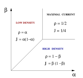
Figure 2: The phase diagram of the TASEP as a function of the boundary rates.

III Current fluctuations for the TASEP

Many properties of the ASEP have been understood using different techniques (Matrix Ansatz, Bethe Ansatz, Random Matrices) MartinReview ; DerridaRep ; FerrariPatrick ; OGKM ; PaulK ; Sasamoto ; Schutzrev ; Spohn ; Zia . However, the determination of current fluctuations in the original TASEP model with open boundaries has remained a vexing and challenging unsolved problem. This question is interesting and important: first, in presence of reservoirs, the model is quite realistic and can be related to real experimental situations Flindt ; VonOppen (a more detailed discussion can be found in Doucot ); second, the exact calculation of fluctuations to all order is akin to determining the large-deviations of the current which are expected to play a central role in non-equilibrium statistical mechanics DerrReview ; Touchette .

III.1 Statement of the problem

We consider the TASEP with open boundaries and want to study the total (i.e., time-integrated) current that has flown through it in the long time limit. One way to quantify this total current is to place a counting variable $N_{t}$ at the entrance site. At $t=0$ we have $N_{0}=0$; each time a particle enters the system, we increment the value of $N_{t}$ by 1. Hence, $N_{t}$ is a random variable that counts the total number of particles that have entered the TASEP between time 0 and $t$. Because the size $L$ is bounded and no particles are created or destroyed in the bulk, $N_{t}$ also represents, when $t\to\infty$, the number of particles that have crossed any bond in the system, or have exited from the TASEP from its right boundary. We call $N_{t}$ the total current at time $t$ and we intend to study its statistical properties.

When $t\to\infty$, the expectation value of $N_{t}/t$ converges towards the average stationary current $J$:

$$\lim_{t\to\infty}\frac{\langle N_{t}\rangle}{t}=J(\alpha,\beta,L)=\frac{Z_{L-1}}{Z_{L}}\,.$$ (5)

The value of $Z_{L}$, defined in equation (4), was determined exactly in DEHP using the Matrix Ansatz.

The variance of $N_{t}$ in the long time limit also increases linearly with time. This allows to define a ‘diffusion-constant’ $\Delta$, as follows:

$$\lim_{t\to\infty}\frac{\langle N_{t}^{2}\rangle-\langle N_{t}\rangle^{2}}{t}=\Delta(\alpha,\beta,L)\,.$$ (6)

An exact expression for $\Delta(\alpha,\beta,L)$ was obtained in DEMal . It involved an extension of the matrix method to represent some two-time correlations in the stationary state. For $\alpha=\beta=1$, the formula for $\Delta$ is quite elegant and involves simple factorial factors (see the next section). Unfortunately, the general result is somehow less compact (see equations (58) to (61) in DEMal ).

More generally, one can define moments and cumulants to all orders for the random variable $N_{t}$. This data can be encoded in the exponential generating function $\langle\exp(\gamma\,N_{t})\rangle.$ The moments of $N_{t}$ are obtained by taking successively the derivatives of this function at $\gamma=0$. In the long-time limit, we have

$$\langle\exp(\gamma\,N_{t})\rangle\simeq\exp(E(\gamma)t)\,.$$ (7)

(A mathematical equality is obtained by taking the logarithm of both sides, dividing by $t$ and taking $t\to\infty$). The derivation of this result is recalled in Section IV. Because the logarithm of $\langle\exp(\gamma\,N_{t})\rangle$ generates the cumulants of $N_{t}$, we observe that these cumulants grow linearly with time and that their values are given by the derivatives of $E(\gamma)$ at $\gamma=0$. The cumulant generating function $E(\gamma)$ is related to the large-deviation function of the current by Laplace transform. For finite-size systems, both functions carry the same information.

The function $E(\gamma)$ was calculated for the symmetric exclusion process in Doucot . Very recently, the analysis of the Bethe Ansatz equations, for $L\to\infty$ was carried out for the asymmetric case, in the low and in the large density phases deGierNew . In the present work, we obtain an explicit representation of the generating function of the cumulants of the current for all values of $\alpha$ and $\beta$ and for all values of the system size $L$. The technique used is an extension of the matrix method (see section IV).

For pedagogical reasons we shall first discuss the case $\alpha=\beta=1$, which belongs to the maximal current phase. Here, the formulae are explicit, quite simple and appealing. The general case with arbitrary values of $(\alpha,\beta)$ will be presented in a separate subsection.

III.2 The cumulant generating function for $\alpha=\beta=1$

Here, we consider the values $\alpha=\beta=1$. Historically, the TASEP with $\alpha=\beta=1$ was the first case for which the stationary measure was determined exactly DeDoMuk . For the cumulants of the current, these special values lead to simple mathematical expressions.

The generating function of the cumulants $E(\gamma)$ is given as a function of $\gamma$ through the following representation in terms of a parameter $B$:

$$\gamma = -\sum_{k=1}^{\infty}\frac{(2k)!}{k!}\frac{[2k(L+1)]!}{[k(L+1)]!\,[k(L+2)]!}\frac{B^{k}}{2k}\,\,,$$ (8)

$$E = -\sum_{k=1}^{\infty}\frac{(2k)!}{k!}\frac{[2k(L+1)-2]!}{[k(L+1)-1]!\,[k(L+2)-1]!}\frac{B^{k}}{2k}\,\,.$$ (9)

By expressing $B$ in terms of $\gamma$ in equation (8) and substituting in equation (9) we can calculate $E$ as a function of $\gamma$ to any desired order. The coefficients of this expansion that we denote by

$$E(\gamma)=E_{1}\gamma+\frac{E_{2}}{2!}\gamma^{2}+\frac{E_{3}}{3!}\gamma^{3}+\ldots,,$$ (10)

give the successive cumulants of $N_{t}$ in the long time limit. For example, we obtain

$$\lim_{t\to\infty}\frac{\langle N_{t}\rangle}{t}=J=E_{1}=\frac{L+2}{2(2L+1)}\,.$$ (11)

This expression is identical to that found in DEHP . When $L\to\infty$, $J\to 1/4$ as expected in the maximal current phase. At the second order, we obtain

$$\lim_{t\to\infty}\frac{\langle N_{t}^{2}\rangle-\langle N_{t}\rangle^{2}}{t}=\Delta=E_{2}=\frac{3}{2}\frac{(4L+1)![L!(L+2)!]^{2}}{[(2L+1)!]^{3}(2L+3)!}\,.$$ (12)

This is the same formula as the one derived in DEMal . When $L\to\infty$, we have $\Delta\simeq\frac{3\sqrt{2\pi}}{64}L^{-1/2}$ i.e., the diffusion constant vanishes in the maximal current phase.

The third cumulant, known as the skewness, is given by:

$$E_{3}=12\,\frac{[(L+1)!]^{2}[(L+2)!]^{4}}{(2L+1)[(2L+2)!]^{3}}\,\Big{\{}9\frac{(L+1)!(L+2)!(4L+2)!(4L+4)!}{(2L+1)![(2L+2)!]^{2}[(2L+4)!]^{2}}-20\frac{(6L+4)!}{(3L+2)!(3L+6)!}\Big{\}}\,.$$ (13)

This formula was not known before. For a large system, the skewness behaves as

$$E_{3}\simeq\frac{2187-1280\sqrt{3}}{10368}\,\pi\sim-0.0090978...$$ (14)

Carrying on the elimination of $B$, the next few orders can also be found explicitly. It is found that the $k$-th cumulant scales as $\pi(\pi L)^{k/2-3/2}$ for $k\geq 2$. We determined the constant prefactor for the first few values of $k$.

The fact that the large deviation function is obtained in parametric form should not come as a surprise. On the contrary, this structure seems to be rather common: to our knowledge it appeared first in DLeb , where the exact large deviation function for the TASEP on a ring was calculated by Bethe Ansatz; it also occurred in the case of a defect particle on a ring evans . The complete solution for the current fluctuations of the ASEP on a ring involves a tree-structure that is again written parametrically Sylvain4 . More generally, it was shown in Bodineau ; Bodineau1 ; DerrReview that for a large class of non-equilibrium diffusive systems, characterized by a linear conductivity and equilibrium diffusion coefficient, the large deviation function can be expressed through a parametric set of equations.

We observe that the limiting value of the skewness, given in equation (14), is a finite number. More generally, one can construct simple ratios of cumulants that have a finite limit when $L\to\infty$. It should be possible to ‘measure’ such numbers in simulations and to test the universality of these ratios in a manner similar to Appert .

III.3 The general case

We now give the result for the cumulant generating function, valid for any system size $L$ and for arbitrary values of $\alpha$ and $\beta$. The mathematical structure is the same as above:

$$\gamma = -\sum_{k=1}^{\infty}C_{k}(\alpha,\beta)\frac{B^{k}}{2k}\,\,,$$ (15)

$$E = -\sum_{k=1}^{\infty}D_{k}(\alpha,\beta)\frac{B^{k}}{2k}\,\,.$$ (16)

The coefficients $C_{k}$ and ${D_{k}}$ of the series are functions of the rates $\alpha$ and $\beta$ and of $L$. Their explicit expressions are given by

$$C_{k}(\alpha,\beta) = \oint_{\{0,a,b\}}\frac{dz}{2i\pi}\frac{F(z)^{k}}{z}$$ (17)

$$\hbox{ and }\,\,\,D_{k}(\alpha,\beta) = \oint_{\{0,a,b\}}\frac{dz}{2i\pi}\frac{F(z)^{k}}{(1+z)^{2}}$$ (18)

where the rational function $F(z)$ is given by

$$F(z)=\frac{-(1+z)^{2L}(1-z^{2})^{2}}{z^{L}(1-az)(z-a)(1-bz)(z-b)}\,\,\,\hbox{ with }a=\frac{1-\alpha}{\alpha}\,\,\hbox{ and }\,\,b=\frac{1-\beta}{\beta}\,.$$ (19)

Equations (15) to (19) provide an exact representation for the generating function of the cumulants of the current in the TASEP with open boundaries. These equations are valid for any system size $L$ and for arbitrary values of the parameters $\alpha$ and $\beta$. Before we proceed further, we explain the meaning of the symbol $\oint_{\{0,a,b\}}$: it represents the complex integral along 3 infinitesimal contours that encircle the points 0, $a$ and $b$ in the complex plane. Equivalently, using the Cauchy formula we could have written equations (17) and (18) as

$$C_{k}(\alpha,\beta) = \sum_{z_{0}=0,a,b}\hbox{Residue}\left[\frac{F(z)^{k}}{z},z_{0}\right]\,\,,$$

$$D_{k}(\alpha,\beta) = \sum_{z_{0}=0,a,b}\hbox{Residue}\left[\frac{F(z)^{k}}{(z+1)^{2}},z_{0}\right]\,.$$

We note that similar integrals have already appeared in closely related problems Cedric ; evans . Here, the notations implicitly assume that $0,a$ and $b$ are distinct. If two or three of these numbers coincide, one should take into account the corresponding residue only once. Hence, for $\alpha=\beta=1$, which implies $a=b=0$, only the residue at 0 must be calculated. The resulting explicit expressions for $C_{k}(1,1)$ and $D_{k}(1,1)$ give the parametric representations (8) and (9) that were discussed in the previous section.

By inverting the series (15) order by order and substituting the result in (16), we can derive closed expressions for the first few cumulants of the current. For example, the mean-value of the current is given by

$$J=\frac{D_{1}(\alpha,\beta)}{C_{1}(\alpha,\beta)}\,.$$ (20)

This formula is, of course, the same as obtained in DEHP . We emphasize that $C_{1}(\alpha,\beta)$ and $D_{1}(\alpha,\beta)$ coincide with $Z_{L}$ and $Z_{L-1}$, respectively, as can be seen by comparing equations (17) and (18) for $k=1$ with equation (B10) of Reference DEHP (see remark ).

At second order we obtain an expression for the diffusion constant

$$\Delta=\frac{D_{1}\,C_{2}-D_{2}\,C_{1}}{C_{1}^{3}}\,.$$ (21)

We remark that $C_{2}$ and $D_{2}$ are natural generalisations of $C_{1}$ and $D_{1}$. In this form, the diffusion constant looks more compact than the formula found in DEMal . The two expressions must coincide but we have not endeavored to prove this fact analytically for all values of $\alpha,\beta$ and $L$. We can carry on this procedure further to a few more orders to obtain higher cumulants and we did so with the help of a symbolic mathematical calculation tool.

It is of greater interest to analyse the behaviour of the large-deviation function in the different phases of the model when $L\to\infty$.

• In the Maximal Current phase, with $\alpha>1/2$ and $\beta>1/2$, the parameters $a$ and $b$ lie inside the unit circle. Hence, the contour integrals that appear in equations (17) and  (18) can be replaced by a single integral along the unit circle. Then, we apply the saddle-point method to estimate the asymptotic behaviour of $C_{k}$ and $D_{k}$ when $L\to\infty$. The saddle point is at $z=1$ and we observe that the values of $a$ and $b$ do not influence the saddle-point estimation at dominant order: in fact they contribute by the same multiplicative factor $[(1-a)(1-b)]^{2k}$, that can be reabsorbed in the parameter $B$. Therefore, the behaviour of the cumulants in the large $L$ limit does not depend on the boundary rates $\alpha$ and $\beta$ in the Maximal Current phase (as expected). The results at dominant order are the same as those obtained for $\alpha=\beta=1$, the special case discussed in the previous section.

• In the Low Density phase, $\alpha<\min(\beta,1/2)$, the parameter $a$ is outside the unit circle, we have $a>b$ and the position of $b$ with respect to the unit circle is not determined. In the large $L$ limit, it is the pole at $z=a$ that contributes dominantly to the values of $C_{k}$ and $D_{k}$ and the parametric representation (15) and (16) becomes (see the appendix for more details)

  $$\gamma = -\sum_{k=1}^{\infty}B^{k}\frac{1}{k!}\frac{d^{k-1}}{dz^{k-1}}\Big{\{}\frac{\phi^{k}(z)}{z}\Big{\}}\Big{|}_{z=a}$$ (22)

  $$E = -\sum_{k=1}^{\infty}B^{k}\frac{1}{k!}\frac{d^{k-1}}{dz^{k-1}}\Big{\{}\frac{\phi^{k}(z)}{(z+1)^{2}}\Big{\}}\Big{|}_{z=a}\,,$$ (23)

  where the function $\phi(z)$ is given by

  $$\phi(z)=(z-a)F(z)=\frac{-(1+z)^{2L}(1-z^{2})^{2}}{z^{L}(1-az)(1-bz)(z-b)}\,.$$ (24)

  These expressions can be used to calculate the first few cumulants in the low density phase:

  $$E_{1} = \rho(1-\rho)\,$$

  $$E_{2} = \rho(1-\rho)(1-2\rho)\,$$

  $$E_{3} = \rho(1-\rho)(1-6\rho+6\rho^{2})\,$$

  $$E_{4} = \rho(1-\rho)(1-2\rho)(1-12\rho+12\rho^{2})$$

  $$E_{5} = \rho(1-\rho)(1-30\rho+150\rho^{2}-240\rho^{3}+120\rho^{4})\,\,\hbox{etc...}$$ (25)

  with the mean density $\rho=\alpha$.

  In fact, using equations (22) and (23), the function for $E(\gamma)$ can be obtained in a closed form thanks to the Lagrange Inversion Formula Flajolet , as explained in the appendix. This leads to

  $$E(\gamma)=\frac{a}{a+1}\frac{{\rm e}^{\gamma}-1}{{\rm e}^{\gamma}+a}\,.$$ (26)

  This expression is identical in the TASEP case to the one obtained by Bethe Ansatz in deGierNew . (In deGierNew , the general PASEP is studied: this adds a prefactor $(p-q)$ to (26), where $p$ and $q$ are the rates of forward and backward jumps, respectively, and modifies the definition of $a$). We remark that the limit formula (26) is rather simple and that it is totally independent of the specific form of the function $\phi(z)$, as can be seen from the derivation given in the appendix. An elementary and physical derivation of this result can be given by using macroscopic fluctuation theory BoDerr ; DerrPriv .

• The High Density phase is symmetrical to the low density phase under the exchange of $\alpha$ and $\beta$. Therefore a separate discussion is not required.

• The shock line $\alpha=\beta\leq 1/2$, i.e., $a=b\geq 1$ can also be analyzed from our general formula. We have calculated explicitly the first few cumulants and obtained the following scaling behaviour

  $$E_{k}\simeq\epsilon_{k}\alpha(1-\alpha)(1-2\alpha)^{k-1}L^{k-2}\hbox{ for }\,k\geq 2\,.$$

  We recall that the current is given by $E_{1}=\alpha(1-\alpha)$. The numerical coefficients are given by $\epsilon_{2}=2/3$, $\epsilon_{3}=-1/30$, $\epsilon_{4}=2/315$, $\epsilon_{5}=-1/1890$… The fact that the higher cumulants grow without bounds with $L$ whereas they are bounded in low and high density phases may come as a surprise. However, it is known that in the shock phase, particles have a vanishing chemical potential and the equivalence between canonical and grand-canonical descriptions breaks down km ; Speer .

  More precisely, this puzzling scaling can be understood from the domain-wall picture, introduced in DEMal to describe the discontinuity by a factor $2/3$ in the diffusion-constant along the shock line. In the limiting case $\alpha=\beta\ll 1$, the dominant configurations are shock profiles between a low density region with $\rho_{l}=\alpha$ and a high density region with $\rho_{h}=1-\beta$. The shock is localized on a single site. The dynamics becomes equivalent to that of a symmetric random walker on a lattice of $L+1$ sites and confined by two reflecting boundaries. The number of particles having entered the TASEP corresponds to the number of leftward steps of the shock. The statistics of the steps performed by an effective random walker between two reflecting walls is a well-posed problem that can be studied independently. For instance, we find that the skewness (third cumulant) of the random walker grows as $-L/30$. However, if we introduce some bias in the jumping rates (which corresponds to the high or low density phase) the walker becomes localized near one of the walls and all cumulants remain finite when $L\to\infty$. Finally, the $\epsilon_{k}$’s can be calculated by remarking that the random walker between two reflecting walls can be mapped to the TASEP with 2 identical particles on a periodic lattice, and then using the results of DLeb .

IV Outline of the Analytical Procedure

We now describe briefly how the expressions (15) to (19) were obtained. Detailed explanations are deferred to a forthcoming article.

IV.1 General setup

In order to study the statistics of $N_{t}$, the total number of particles that have entered into the system, one introduces the joint distribution $P_{t}({\mathcal{C}},N)$, the probability of being at time $t$ in configuration ${\mathcal{C}}$ and having $N_{t}=N$. The evolution equation of $P_{t}({\mathcal{C}},N)$ can be written using the Markov equation (1). It is then useful to introduce the Laplace transform DLeb ; OGKM

$$F_{t}({\mathcal{C}})=\sum_{N}{\rm e}^{\gamma N}P_{t}({\mathcal{C}},N)\,.$$

These generalized weights satisfy a deformed Markov equation

$$\frac{dF_{t}}{dt}=M(\gamma)F_{t}\,.$$ (27)

The matrix $M(\gamma)$ of size $2^{L}$ is given by

$$M(\gamma)=M+({\rm e}^{\gamma}-1)M_{1}\,,$$ (28)

where $M$ is the original Markov operator and the matrix $M_{1}$ contains only those transitions in which a particle enters the system, i.e., $M_{1}({\mathcal{C}},{\mathcal{C}^{\prime}})=\alpha$ if ${\mathcal{C}^{\prime}}$ evolves into ${\mathcal{C}}$ by adding a particle at site 1 and $M_{1}({\mathcal{C}},{\mathcal{C}^{\prime}})=0$ otherwise. Equation (27) is formally solved as $F_{t}=\exp(M(\gamma)t)F_{0}$ which, in the long time limit, behaves as

$$F_{t}\simeq{\rm e}^{E(\gamma)t}\,|E(\gamma)\rangle\,,$$

where $E(\gamma)$ is the dominant eigenvalue of $M(\gamma)$ and $|E(\gamma)\rangle$ the associated eigenvector (it is unique for sufficiently small $\gamma$). Thus, we obtain equation (7)

$$\langle\exp(\gamma\,N_{t})\rangle=\sum_{{\mathcal{C}}}F_{t}({\mathcal{C}})\simeq\exp(E(\gamma)t)\,.$$

The cumulant generating function is therefore identical to the largest eigenvalue of the deformed operator $M(\gamma)$ and the problem of determining the statistics of $N_{t}$ has been traded for a spectral problem. This question can be tackled using different methods. Bethe Ansatz is one technique for integrable systems. Another approach, valid for small values of $\gamma$, is to perform a perturbative expansion around the dominant eigenvector, $|0\rangle$, and the dominant eigenvalue, $0$, of the original Markov matrix $M$:

$$E(\gamma) = E_{1}\gamma+\frac{E_{2}}{2!}\gamma^{2}+\frac{E_{3}}{3!}\gamma^{3}+\ldots$$

$$|E(\gamma)\rangle = |0\rangle+\gamma|1\rangle+\gamma^{2}|2\rangle+\ldots$$ (29)

Carrying out the perturbative expansion explicitly, we find that the $k$-th order correction to the eigenvector satisfies an equation of the type

$$M|k\rangle={\mathcal{R}}_{k}\left(|0\rangle,\ldots|k-1\rangle\right)\,,$$ (30)

${\mathcal{R}}_{k}$ being a linear functional. For example, we have

$$M|0\rangle=0\,,\,\,\,\,M|1\rangle=(E_{1}-M_{1})|0\rangle\quad\hbox{etc ...}$$

Moreover, the solvability condition (obtained by using the fact that vector $\langle 0|=(1,1,\ldots,1)$ is the left null-eigenvector of the Markov matrix $M$) allows to express the $k$-th term in $E(\gamma)$ (i.e., the cumulant of order $k$) as a linear function of the $k-1$ vectors $|1\rangle,|2\rangle,\ldots|k-1\rangle$. For example, we have

$$E_{1}=\langle 0|M_{1}|0\rangle\,,\,\,\,\,\,E_{2}=2\langle 0|M_{1}|1\rangle+(1-2E_{1})\langle 0|1\rangle\quad\hbox{etc...}$$ (31)

The cumulants of the current can be found if we are able to solve the set of linear equations (30) for all values of $k\geq 0$. At order 0, the stationary state $|0\rangle$ and the mean current $E_{1}$ were calculated thanks to the Matrix Ansatz, recalled in equations  (2) (3) and (4). In DEMal , the first order correction was also obtained by a Matrix Ansatz: the required algebra was constructed by taking tensor products of two quadratic algebras of the type (3). This allowed to calculate the diffusion constant $E_{2}$.

IV.2 Steps of the calculations and Numerical tests

The computations that we have carried out can be summarized by the following steps:

(i) The Matrix Ansatz used in DEMal has been simplified and generalized to all orders. The operators required to calculate the $(k+1)$-th cumulant are denoted by ${\bf D}_{k}$ and ${\bf E}_{k}$. These operators are constructed by using $2k+1$ tensor products of the original ${\bf D}$ and ${\bf E}$’s. This may appear daunting at first sight but in fact this is not so bad: the ${\bf D}_{k}$ and ${\bf E}_{k}$ already appear in the studies of multispecies exclusion processes EFM ; MMR ; Sylvain4 . There they were introduced as formal objects to construct the stationary measure. Here, they are used as tools for calculations. We have also found the boundary vectors ${\bf\langle\alpha_{k}|}$ and ${\bf|\beta_{k}\rangle}$.

(ii) The fact that ${\bf D}_{k}$ and ${\bf E}_{k}$ allow to solve the system (30) at each order has been proved recursively. Using the relations (31), an expression for the cumulant $E_{k}$ in terms of matrix elements involving ${\bf D}_{k}$ and ${\bf E}_{k}$ and the previously determined $E_{j}$’s for $j<k$ can be written.

(iii) The next step is to calculate the matrix elements. Typically, one has to determine a ‘normalization’-type term $\langle\alpha_{k}|({\bf D}_{k}+{\bf E}_{k})^{L}|\beta_{k}\rangle$ that generalizes (4). Such a matrix element can be found by using the image method DEMal ; MartinNotes in a space of dimension $2k+1$. The resulting expression involves sums of products of binomial factors. These binomial factors can be expressed as multiple contour integrals and the total sum can be recast as a determinant. As this stage, the cumulants are written as complex integrals over determinantal expressions.

(iv) The diffusion constant ($k=2$) was recalculated. The skewness ($k=3$) was then determined by evaluating the contour integrals. These integrals produce a ‘generic’ term and a very large number of boundary terms. It was found that the global contribution of the boundary terms cancels out for $k=2$ and 3. It was also observed that a parametric expression for $\gamma$ and $E$ at order 3 as a function of an arbitrary parameter $B$ allows to retrieve the diffusion constant and the skewness.

(v) At $k$-th order, a calculation of the ‘generic’ term was performed by assuming that the various contributions of boundary terms globally cancel out. It was observed that the resulting formula could also be obtained through the parametric expressions (15) and (16) for $\gamma$ and $E$ at order $k$ with respect to $B$, that were guessed at all orders.

We admit that our final result was guessed rather than fully worked out. The gaps in our derivations (steps (iv) and (v)) have to be filled. However, we emphasize that we have been using a systematic procedure and that we are absolutely sure that the equations (15) to (19) are correct. We have tested numerically the conjectured formulae in the following cases:

• For $\alpha=\beta=1$, the formula (13) for the skewness was compared with the exact result obtained by solving the linear equations (30) for the first three orders for systems of sizes $L\leq 10$. The results agreed in all cases. The expressions are rational numbers which involve integers having more than 20 digits.

• For $\alpha=\beta=1$, the first 6 cumulants were verified for $L\leq 10$.

• The formula for the second cumulant (21) as a function of $\alpha$ and $\beta$ was tested against the exact result for $L=4$.

• We have chosen arbitrary values of $\alpha$ and $\beta$ throughout the phase diagram (a dozen of different cases). By taking rational values for $\alpha$ and $\beta$, we insure that the formal mathematical program (Mathematica) performs exact calculations on integers when solving the linear equations (30). We have worked with systems of size $L\leq 10$ and tested the formula up to the 6th cumulant. The integers that appear involve hundreds of digits (450 in the worst chosen case): the expressions (15) to (19) give the correct answer in all cases.

Finally, we emphasize the formulae given here allow us to re-derive results that were known previously, such as equations (12) and (26). This provides an indirect verification of their correctness.

V Discussion

In the present work, we give closed formulae for the generating function of the cumulants of the current in the open TASEP. These results hold for all values of the boundary parameters $\alpha$ and $\beta$ and all values of the system size $L$. We emphasize the fact that our expressions are exact and not only asymptotic: they are of combinatorial nature. They allow us to describe the ASEP at all points of its phase diagram, including the phase-transition lines. The cumulant generating function is given in the form of a parametric representation – equations  (15) to (19): a similar mathematical structure can be found in other works DLeb ; evans ; Sylvain4 and it can be related physically to the additivity principle Bodineau ; DerrReview .

The statistics of the current in the open TASEP had remained a challenging open problem for many years and no exact solution for the full distribution of the current was known for finite size systems. The Bethe Ansatz equations for the open ASEP were studied in deGier1 but they are valid only on some surfaces in the parameter space: this restriction seemed to be a major obstruction to the computation of the large-deviation function. Only recently, a very subtle analysis of the Bethe equations, valid in the $L\to\infty$ limit, together with some conjectures on the asymptotic locations of the Bethe roots, was carried out in deGierNew , leading to an expression for the cumulant generating function. However, the result in deGierNew can only be established deep inside the low and the high density phases and it is an asymptotic expression, valid only when $L\to\infty$. In our work, we have followed a different path and used the Matrix Product Representation DEHP ; MartinReview to calculate the cumulants of the current order by order. We have performed some explicit calculations and uncovered the general structure of the solution. From the mathematical point of view, our formulae are only a conjecture but we have verified it in dozens of cases and derived from it all the previously known results. We have absolutely no doubt that our expressions are true. In particular, the main expression obtained in deGierNew can be derived as a limiting case of our results.

We have decided to present the final formulae before completing the proof, because we find the results elegant and sufficient by themselves. Furthermore, they allow to draw some interesting physical consequences and to open new problems. We think that the proof is a question of carrying out a very long computation rather than having some deep mathematical insight. We are presently working on this aspect. We hope to have given enough details to the reader to clarify what kind of assumptions were made, that allowed us to jump to the final result and to guess the full structure of the solution. Another possibility, now that the final formula is known, is to search for a direct method to check it: after all, the cumulant generating function is nothing but the largest eigenvalue of a known operator.

Besides completing the derivation, we also intend to extract from equations (15) to (19) the scaling limit of the large deviation function in the $L\to\infty$ limit. It would be interesting to compare that scaling form with recent numerical results obtained by Monte-Carlo and DMRG methods Gorissen ; Mitsudo ; Proeme and also to investigate the crossover with theoretical results derived on the infinite lattice FerrariPatrick ; Sasamoto .

Finally, we have considered here only the TASEP. But the matrix method can also be applied to the partially asymmetric case (PASEP), and we have checked that tensor products of the PASEP quadratic algebra that appeared in multispecies PASEP models PEM allow us to solve the hierarchy of equations (30) for the cumulants. We believe that the parametric representation still holds in the PASEP case and that combinatorial tree-structures akin to those found for the PASEP on a periodic ring in Sylvain4 will probably play an important role. Besides, complex integral representations for matrix elements analogous to those we have used here also appear in the PASEP MartinReview ; MartinPASEP ; SasaPasep1 ; SasaPasep2 . There must exist a general and hopefully elegant structure that encompasses all the cases, though we are well aware that such a structure may be difficult to discover.

We acknowledge interesting discussions with O. Golinelli, S. Prolhac and R. Vasseur. We are grateful to S. Mallick for a very careful reading of the manuscript and P. Krapivsky for useful remarks. We are thankful to B. Derrida for telling us how to obtain equation (26) from macroscopic fluctuation theory.

Appendix A Derivation of equation (26)

Let $C_{0}$,$C_{a}$ and $C_{b}$ be three infinitesimal contours (circles) that surround the points $0$, $a$ and $b$ in the complex plane. According to equations (17) and (18), we must calculate contour integrals along these three circles. We denote by $\Gamma_{1}$ the unit circle.

In the low density phase $\alpha<\min(\beta,1/2)$, the parameter $a$ is outside the unit disk and we have $a>b$. The point $b$ can be either inside or outside the unit disk. In order to perform a saddle-point analysis in the large $L$ limit, a contour must pass through the point $z=1$. We therefore deform the infinitesimal contour $C_{0}$ encircling 0 into the unit circle $\Gamma_{1}$. But then we must remove the contribution of the pole $1/a$ of $F(z)$ which is inside $\Gamma_{1}$ (see figure 3). We must also distinguish the cases $b<1$ or $b>1$: For $b<1$ we can write, formally: $C_{0}+C_{a}+C_{b}=\Gamma_{1}-C_{1/a}+C_{a}$. For $b>1$ we can write $C_{0}+C_{a}+C_{b}=\Gamma_{1}-C_{1/a}-C_{1/b}+C_{a}+C_{b}$. Now the function $F$ satisfies: $F(z)=F(1/z)$. Thus for $z_{0}=a,b$, we have

$$\hbox{Residue}\left[\frac{F(z)^{k}}{z},z_{0}\right] = -\hbox{Residue}\left[\frac{F(z)^{k}}{z},1/z_{0}\right]$$

$$\hbox{Residue}\left[\frac{F(z)^{k}}{(z+1)^{2}},z_{0}\right] = -\hbox{Residue}\left[\frac{F(z)^{k}}{(z+1)^{2}},1/z_{0}\right]\,.$$ (32)

Formally this can be written as $C_{1/a}=-C_{a}$ and $C_{1/b}=-C_{b}$. Finally the contours for the complex integrals reduce to $\Gamma_{1}+2C_{a}$ if $b<1$ and to $\Gamma_{1}+2C_{a}+2C_{b}$ if $b>1$.

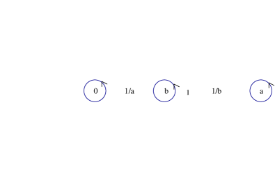
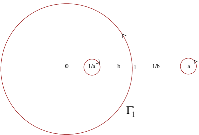
Figure 3: The two sets of equivalent contours in the complex plane. In this figure, we have supposed that $b$ lies inside the unit disk.

The integral over $\Gamma_{1}$ is estimated by saddle point: it is of order $4^{L}$. The integral over $C_{a}$ is of order $(2+a+1/a)^{L}\gg 4^{L}$ (because $a>1$). The residue at $b$ contributes only when $b>1$ but in that case it is of order $(2+b+1/b)^{L}\ll(2+a+1/a)^{L}$ (because $b<a$). Hence, in all cases, in the large $L$ limit, the dominant contribution comes from the contour around $a$, which has to be counted twice. Finally, using Cauchy’s formula, we can write

$$C_{k}(\alpha,\beta)=2\oint_{C_{a}}\frac{dz}{2i\pi}\frac{(\phi(z)^{k}/z)}{(z-a)^{k}}=\frac{2}{(k-1)!}\frac{d^{k-1}}{dz^{k-1}}\left\{\left(\phi(z)\right)^{k}\frac{1}{z}\right\}\Big{|}_{z=a}$$ (33)

where the function $\phi(z)$ has been defined in (24). Similarly, we have

$$D_{k}(\alpha,\beta)=\frac{2}{(k-1)!}\frac{d^{k-1}}{dz^{k-1}}\left\{\left(\phi(z)\right)^{k}\frac{1}{(z+1)^{2}}\right\}\Big{|}_{z=a}\,.$$ (34)

Substituting these expressions into the formulae (15) and (16) leads to equations (22) and (23).

We now need the Lagrange Inversion formula Flajolet , that can be stated as follows. Suppose that the two complex variables $z$ and $w$ are related in terms of the parameter $B$ as

$$w=z+B\phi(w)$$ (35)

where $\phi$ is locally analytic. Then, any function $G(w)$ can be expanded as a power-series in $B$ as follows:

$$G(w)=G(z)+\frac{B}{1!}\phi(z)G^{\prime}(z)+\frac{B^{2}}{2!}\frac{d}{dz}\left\{\left(\phi(z)\right)^{2}G^{\prime}(z)\right\}+\ldots+\frac{B^{n+1}}{(n+1)!}\frac{d^{n}}{dz^{n}}\left\{\left(\phi(z)\right)^{n+1}G^{\prime}(z)\right\}+\ldots$$ (36)

We can identify the expression (22) for $\gamma$ with the Lagrange’s Inversion formula applied at the point $z=a$ with $G(z)=-\log(z)$. We obtain

$$\gamma=-\log(w)+\log(a)\,.$$ (37)

We can also compare Lagrange’s Inversion formula with the expression (23) for $E$, taking now $G(z)=\frac{1}{z+1}$. We obtain

$$E=\frac{1}{w+1}-\frac{1}{a+1}\,.$$ (38)

Eliminating $w$ between the last two equations leads to the desired expression (26). We note that the precise form of $\phi(z)$ has played no role. This suggest that the formula (26) for the cumulant generating function should be rather universal.

References

- (1) R. A. Blythe and M. R. Evans, 2007, Nonequilibrium steady states of matrix-product form: a solver’s guide, J. Phys. A: Math. Theor. 40, R333.
- (2) R. A. Blythe, M. R. Evans, F. Colaiori and F. H. L. Essler, 2000, Exact solution of a partially asymmetric exclusion model using a deformed oscillator algebra, J. Phys. A: Math. Gen. 33, 2313.
- (3) T. Bodineau, B. Derrida, 2004, Current fluctuations in nonequilibrium diffusive systems: An additivity principle, Phys. Rev. Lett. 92, 180601.
- (4) T. Bodineau, B. Derrida, 2005, Distribution of currents in non-equilibrium diffusive systems and phase transitions, Phys. Rev. E 72, 066110.
- (5) T. Bodineau, B. Derrida, 2006, Current large deviations for asymmetric exclusion processes with open boundaries, J. Stat. Phys. 123, 277.
- (6) C. Boutillier, P. François, K. Mallick and S. Mallick, 2002, A matrix Ansatz for the diffusion of an impurity in the asymmetric exclusion process, J. Phys. A: Math. Gen. 35, 9703.
- (7) J. de Gier, F. H. L. Essler, 2005, Bethe Ansatz solution of the Asymmetric Exclusion Process with Open Boundaries, Phys. Rev. Lett. 95, 240601.
- (8) J. de Gier, F. H. L. Essler, 2011, Current large deviation function for the open asymmetric simple exclusion process, arXiv:1011.3235.
- (9) B. Derrida, 1998, An exactly soluble non-equilibrium system: the asymmetric simple exclusion process, Phys. Rep. 301, 65.
- (10) B. Derrida, 2007, Non-equilibrium steady states: fluctuations and large deviations of the density and of the current, J. Stat. Mech.: Theor. Exp. P07023.
- (11) B. Derrida, 2011, Private communication.
- (12) B. Derrida and C. Appert, 1999, Universal Large-Deviation Function of the Kardar-Parisi-Zhang Equation in One Dimension, J. Stat. Phys. 94, 1.
- (13) B. Derrida, E. Domany and D. Mukamel, 1992 An exact solution of a one-dimensional asymmetric exclusion model with open boundaries, J. Stat. Phys. 69, 667.
- (14) B. Derrida, B. Douçot and P.-E. Roche, 2004, Current fluctuations in the one-dimensional symmetric exclusion process with open boundaries, J. Stat. Phys. 115 717.
- (15) B. Derrida, M. R. Evans, 1999, Bethe Ansatz solution for a defect particle in the asymmetric exclusion process, J. Phys. A: Math. Gen. 32, 4833.
- (16) B. Derrida, M. R. Evans, V. Hakim, V. Pasquier, 1993, Exact solution of a 1D asymmetric exclusion model using a matrix formulation, J. Phys. A: Math. Gen. 26, 1493.
- (17) B. Derrida, M. R. Evans and K. Mallick, 1994, Exact Diffusion Constant of a One-Dimensional Asymmetric Exclusion Model with Open Boundaries, J. Stat. Phys. 79, 833.
- (18) B. Derrida, J. L. Lebowitz, 1998, Exact large deviation function in the asymmetric exclusion process, Phys. Rev. Lett. 80, 209.
- (19) M. R. Evans, 1994, Unpublished Notes.
- (20) M. R. Evans, P. A. Ferrari and K. Mallick, 2009, Matrix Representation of the Stationary Measure for the Multispecies TASEP, J. Stat. Phys. 135, 217.
- (21) P. L. Ferrari, 2010, From Interacting particle systems to random matrices, arXiv:1008.4853.
- (22) P. Flajolet and R. Sedgewick, 2009, Analytic Combinatorics, (Cambridge University Press, Cambridge).
- (23) C. Flindt, T. Novotný and A.-P. Jauho, 2004, Current noise in vibrating quantum array, Phys. Rev. B 70, 205334.
- (24) O. Golinelli and K. Mallick, 2006, The asymmetric exclusion process: an integrable model for non-equilibrium statistical mechanics, J. Phys. A: Math. Gen. 39, 10647.
- (25) M. Gorissen and C. Vanderzande, 2010, Finite size scaling of current fluctuations in the totally asymmetric exclusion process, arXiv:1010.5139.
- (26) S. A. Janowsky and J. L. Lebowitz, 1992, Finite-size effects and shock fluctuations in the asymmetric simple-exclusion process, Phys. Rev. A 45, 618.
- (27) T. Karzig and F. von Oppen, 2010, Signatures of critical full counting statistics in a quantum-dot chain, Phys. Rev. B 81, 045317.
- (28) J. Krug, 1991, Boundary-induced phase transitions in driven diffusive systems, Phys. Rev. Lett. 67, 1882.
- (29) K. Mallick, 1996, Shocks in the asymmetry exclusion model with an impurity, J. Phys. A: Math. Gen. 29, 5375.
- (30) K. Mallick, S. Mallick and N. Rajewsky, 1999, Exact solution of an exclusion process with three classes of particles and vacancies, J. Phys. A: Math. Gen. 32, 8399.
- (31) T. Mitsudo and S. Takesue, 2010, The numerical estimation of the current large deviation function in the asymmetric exclusion process with open boundary conditions, arXiv:1012.1387.
- (32) P. L. Krapivsky, S. Redner and E. Ben-Naim, 2010, A Kinetic View of Statistical Physics (Cambridge: Cambridge University Press).
- (33) A. Proeme, R. A. Blythe and M. R. Evans, 2010, Dynamical Transition in the Open-boundary Totally Asymmetric Exclusion Process, arXiv:1010.5741.
- (34) S. Prolhac, 2010, Tree structures for the current fluctuations in the exclusion process, J. Phys. A: Math. Theor. 43, 105002.
- (35) S. Prolhac, M. R. Evans, K. Mallick, 2009, The matrix product solution of the multispecies partially asymmetric exclusion process, J. Phys. A: Math. Theor. 42, 165004.
- (36) N. Rajewsky, T. Sasamoto and E. R. Speer, 2000, Spatial particle condensation for an exclusion process on a ring, Physica A 279, 123.
- (37) T. Sasamoto, 1999, One-dimensional partially asymmetric simple exclusion process with open boundaries: orthogonal polynomial approach, J. Phys. A: Math. Gen. 32, 7109.
- (38) T. Sasamoto, 2000, Density profile of the one-dimensional partially asymmetric simple exclusion process with open boundaries, J. Phys. Soc. Japan 69, 1055.
- (39) T. Sasamoto, 2007, Fluctuations of the one-dimensional asymmetric exclusion process using random matrix techniques, J. Stat. Mech.: Theor. Exp. P07007.
- (40) B. Schmittmann and R. K. P. Zia, 1995, Statistical mechanics of driven diffusive systems, in Phase Transitions and Critical Phenomena vol 17., C. Domb and J. L. Lebowitz Ed., (San Diego, Academic Press).
- (41) G. M. Schütz, 2001, Exactly Solvable Models for Many-Body Systems Far from Equilibrium in Phase Transitions and Critical Phenomena vol 19., C. Domb and J. L. Lebowitz Ed., (Academic Press, San Diego).
- (42) G. M. Schütz and E. Domany, 1993, Phase Transitions in an exactly soluble one-dimensional exclusion process, J. Stat. Phys. 72, 277 (1993).
- (43) H. Spohn, 1991, Large scale dynamics of interacting particles, (Springer-Verlag, New-York).
- (44) H. Touchette, 2009, The large deviation approach to statistical mechanics, Phys. Rep. 478 1.