Landscape encodings enhance optimization

Abstract

Hard combinatorial optimization problems deal with the search for the minimum cost solutions (ground states) of discrete systems under strong constraints. A transformation of state variables may enhance computational tractability. It has been argued that these state encodings are to be chosen invertible to retain the original size of the state space. Here we show how redundant non-invertible encodings enhance optimization by enriching the density of low-energy states. In addition, smooth landscapes may be established on encoded state spaces to guide local search dynamics towards the ground state.

I Introduction

Complex systems in our world are often computationally complex as well. In particular, the class of NP-complete problems Garey and Johnson (1979), for which no fast solvers are known, encompasses not only a wide variety of well-known combinatorial optimization problems from the Travelling Salesman Problem to graph coloring, but also includes a rich diversity of applications in the natural sciences ranging from genetic networks Berg and Lässig (2004) through protein folding Fraenkel (1993) to spin glasses Mézard and Zecchina (2002); Bauer and Orland (2005); Schulman (2007); Ricci-Tersenghi (2010). In such cases, heuristic optimization – where the goal is to find the best solution that is reachable within an allocated time – is widely accepted as being a more fruitful avenue of research than attempting to find an exact, globally optimal, solution. This view is motivated at least in part by the realization that in physical and biological systems, there are severe constraints on the type of algorithms that can be naturally implemented as dynamical processes. Typically, thus, we have to deal with local search algorithms. Simulated annealing Kirkpatrick et al. (1983), genetic and evolutionary algorithms Holland (1992), as well as genetic programming Koza (1992) are the most prominent representatives of this type. Their common principle is the generation of variation by thermal or mutational noise, and the subsequent selection of variants that are advantageous in terms of energy or fitness Reidys and Stadler (2002).

The performance of such local search heuristics naturally depends on the structure of the search space, which, in turn, depends on two ingredients: (1) the encoding of the configurations and (2) a move set. Many combinatorial optimization problems as well as their counterparts in statistical physics, such as spin glass models, admit a natural encoding that is (essentially) free of redundancy. In the evolutionary computation literature this “direct encoding” is often referred to as the “phenotype space”, $X$. The complexity of optimizing a cost function $f$ over $X$ is determined already at this level. For simplicity, we call $f$ energy and refer to its global minima as ground states. In evolutionary computation, one often uses an additional encoding $Y$, called the “genotype space” on which search operators, such as mutation and cross-over, are defined more conveniently Rothlauf and Goldberg (2003); Rothlauf (2006). The genotype-phenotype relation is determined by a map $\alpha:Y\to X\cup\{\varnothing\}$, where $\varnothing$ represents phenotypic configurations that do not occur in the original problem, i.e. non-feasible solutions. For example, the tours of a Traveling Salesman Problem (TSP) Applegate et al. (2006) are directly encoded as permutations describing the order of the cities along the tour. A frequently used encoding as binary strings represents every connection between cities as a bit that can be present or absent in a tour; of course, most binary strings do not refer to valid tours in this picture.

The move set (or more generally the search operators Flamm et al. (2007)) define a notion of locality on $X$. Here we are interested only in mutation-based search, where for each $x\in X$ there is a set of neighbors $N(x)$ that is reachable in a single step. Such neighboring configurations are said to be neutral if they have the same fitness. Detailed investigations of fitness landscapes arising from molecular biology have led to the conclusion that high degrees of neutrality can facilitate optimization Schuster et al. (1994); Reidys and Stadler (2002). More precisely, when populations are trapped in a metastable phenotypic state, they are most likely to escape by crossing an entropy barrier, along long neutral paths that traverse large portions of genotype space van Nimwegen and Crutchfield (2000).

In contrast, some authors advocate to use “synonymous encodings” for the design of evolutionary algorithms, where genotypes mapping to the same phenotype $x\in X$ are very similar, i.e., $\alpha^{-1}(x)$ forms a local “cluster” in $Y$, see e.g. Rothlauf (2006); Choi and Moon (2008); Rothlauf (2011). This picture is incompatible with the advantages of extensive neutral paths observed in biologically inspired landscape models Schuster et al. (1994); Fernández and Solé (2007) and in genetic programming Yu and Miller (2002); Banzhaf and Leier (2006). An empirical study Knowles and Watson (2002), furthermore, shows that the introduction of arbitrary redundancy (by means of random Boolean network mapping) does not increase the performance of mutation-based search. This observation can be understood in terms of a random graph model of neutral networks, in which only very high levels of randomized redundancy result in the emergence of neutral paths Reidys et al. (1997).

An important feature that appears to have been overlooked in most recent literature is that the redundancy of $Y$ with respect to $X$ need not be homogeneous Rothlauf and Goldberg (2003). Inhomogeneous redundancy implies that the size of the preimage $|\alpha^{-1}(x)|$ may depend on $x\in X$. If $|\alpha^{-1}(x)|$ is anti-correlated with the energy $f(x)$, then the encoding $Y$ enables the preferential sampling of low-energy states in $X$. Thus even a random selection of a state yields lower energy when performed in $Y$ than in $X$. Here we demonstrate this enrichment of low energy states for three established combinatorial optimization problems and suitably chosen encodings. The necessary formal aspects of energy landscapes and their encodings are outlined in the Methods section. We formalize and measure enrichment in terms of densities of states on $X$ and $Y$, see Methods for a formal treatment. We illustrate the effects of encoding by comparing performance of optimization heuristics on the direct and encoded landscapes.

II Results and Discussion

II.1 Number Partitioning

The first optimization problem we consider is the number partitioning problem (NPP) Garey and Johnson (1979): this asks if one can divide $n$ positive numbers $a_{1},a_{2},\dots,a_{n}$ into two subsets such that the sum of elements in the first subset is the same as the sum over elements in the other subset. The energy is defined as the deviation from equal sums in the two subsets, i.e.,

$$f(x)=\left|\sum_{i=1}^{n}x_{i}a_{i}\right|$$ (1)

where the two choices $x_{i}\in\{-1,+1\}$ correspond to assignment to the first or to the second subset, respectively. The flipping of one of the spin variables $x_{i}$ is used as a move set, so that the NPP landscape is built on a hypercube. The NPP shows a phase transition between an easy and a hard phase. We consider here only instances that are hard in practice, i.e., where the coefficients $a_{i}$ have a sufficiently large number of digits Mertens (1998).

The so-called prepartitioning encoding Ruml et al. (1996) of the NPP is based on the differencing heuristic by Karmakar and Karp Karmakar and Karp (1982). Departing from an NPP instance $(a_{1},\dots,a_{n})$, the heuristic removes the largest number, say $a_{i}$, and the second largest $a_{j}$ and replaces them by their difference $a_{i}-a_{j}$. This reduces the problem size from $n$ to $n-1$. After iterating this differencing step $n-1$ times, the single remaining number is an upper bound for — and in many cases a good approximation to — the global minimum energy. The minimizing configuration itself is obtained by keeping track of the items chosen for differencing. Replacing $a_{i}$ and $a_{j}$ by their difference amounts to putting $a_{i}$ and $a_{j}$ into different subsets, i.e. $x_{i}\neq x_{j}$.

The prepartitioning encoding is obtained by modifying the initial condition of the heuristic. Each number $a_{i}$ is assigned a class $y_{i}\in\{1,\dots,n\}$. A new NPP instance $a^{\prime}_{1},\dots,a^{\prime}_{n}$ is generated by adding up all numbers $a_{i}$ in the same class $y_{i}$ into a single number $a^{\prime}_{y_{i}}$. After removing zeros from $a^{\prime}$, the differencing heuristic is applied to $a^{\prime}$. In short: $y_{i}=y_{j}$ imposes the constraint $x_{i}=x_{j}$. Running the heuristic under this constraint, the resulting configuration $x=\alpha(y)$ is unique up to flipping all spins in $x$. The so defined mapping $\alpha:Y\rightarrow X$ is surjective because for each $x\in X$, $\alpha(y)=x$ for $y_{i}=1$ if $x_{i}=1$ and $y_{i}=2$ otherwise. Two encodings $y,z\in Y$ are neighbors if they differ at exactly one index $i\in\{1,\dots,n\}$. This encoding is the one whose performance we will compare with the direct encoding later.

II.2 Traveling Salesman

Our next optimization problem, the Traveling Salesman Problem, (TSP) is another classical NP-hard optimization problem Garey and Johnson (1979). Given a set of $n$ vertices (cities, locations) $\{1,\dots,n\}$ and a symmetric matrix of distances or travel costs $d_{ij}$, the task is to find a permutation (tour) $\pi$ that minimizes the total travel cost

$$f(\pi)=\sum_{i=1}^{n}d_{\pi(i),\pi(i+1)}$$ (2)

where indices are interpreted modulo $n$. Here, the states of the landscape are the permutations of $\{1,\dots,n\}$, $X=S_{n}$. Two permutations $\pi$ and $\sigma$ are adjacent, $\{\pi,\sigma\}\in L$, if they differ by one reversal. This means that there are indices $i$ and $j$ with $i<j$ such that $\sigma_{k}=\pi_{i+j-k}$ for $i\leq k\leq j$ and $\sigma_{k}=\pi_{k}$ otherwise.

Similar to the NPP case, an encoding configuration $y\in Y:=\{1,2,\dots,n\}^{n}$ acts as a constraint. A tour $\pi\in X$ fulfills $y$ if for all cities $i$ and $j$, $y_{i}\leq y_{j}$ implies $\pi^{-1}(i)\leq\pi^{-1}(j)$. Thus $y_{i}$ is the relative position of city $i$ in the tour since it must come after all cities $j$ with $y_{j}<y_{i}$. All cities with the same $y$-value appear in a single section along the tour. If there are no two cities with the same $y$-value then $y$ itself is a permutation and there is a unique $\pi\in X$ obeying $y$, namely $\pi=y^{-1}$.

Among the tours compatible with the constraint, a selection is made with the greedy algorithm. It constructs a tour by iteratively fixing adjacencies of cities. Starting from an empty set of adjacencies, we attempt to include an adjacency $\{i,j\}$ at each step. If the resulting set of adjacencies is still a subset of a valid tour obeying the constraint, the addition is accepted, otherwise $\{i,j\}$ is discarded. The step is iterated, proposing each $\{i,j\}$ exactly once in the order of decreasing $d_{i,j}$. This procedure establishes a mapping (encoding) $\alpha:Y\rightarrow X$. Since each tour $\pi$ can be reached by taking $y=\pi^{-1}$, $\alpha$ is complete. In the encoded landscape, two states $y,z\in Y$ are adjacent if they differ at exactly one position (city) $i$.

II.3 Maximum Cut

The last example we consider is a Spin Glass problem. Consider the set of configurations $X=\{-1,+1\}^{n}$ with the energy function

$$f(x)=-\sum_{i,j}J_{ij}x_{i}x_{j}$$ (3)

for a spin configuration $x\in X$. Proceeding differently from the usual Gaussian or $\pm J$ spin glass models Sherrington and Kirkpatrick (1975); Binder and Young (1986), we allow the coupling to be either antiferromagnetic or zero, $J_{ij}\in\{-1,0\}$. This is sufficient to create frustration and obtain hard optimization problems. Taking the negative coupling matrix $-J$ as the adjacency matrix of a graph $G$, the spin glass problem is equivalent to the max-cut problem on $G$, which asks to divide the node set of $G$ into two subsets such that a maximum number of edges runs between the two subsets Garey and Johnson (1979).

The idea for an encoding works on the level of the graph $G$, which we assume to be connected. The set $Y$ of the encoding consists of all spanning trees of $G$. In the mapped configuration $x=\alpha(y)$, $x_{i}$ and $x_{j}$ have different spin values whenever $ij$ is an edge of the spanning tree $y$. Since a spanning tree is a connected bipartite graph, this uniquely (up to $+1/-1$ symmetry) defines the spin configuration $x$. The encoding $\alpha$ is not complete in general. Homogeneous spin configurations, for instance, are not generated by any spanning tree. Each ground state configuration $x_{\text{ground}}$, however, is certain to be represented by a spanning tree due to the following argument. Suppose there is a minimum energy configuration $x_{\text{ground}}$ that is not generated by any spanning tree. Then the subgraph of $G$ formed by all edges connecting unequal spins in $x_{\text{ground}}$ is disconnected. We choose one of the connected components, calling its node set $C$. By flipping all spins in $C$, we keep all edges present for $x_{\text{ground}}$. Since $G$ is connected, we obtain at least one additional edge from a node in $C$ to a node outside $C$. Thus we have constructed a configuration with strictly lower energy than $x_{\text{ground}}$, a contradiction. Two spanning trees $y,z\in Y$ are adjacent, if $z$ can be obtained from $y$ by addition of an edge $e$ and removal of a different edge $f$.

Figure 1: Enrichment of the density of low energy states for landscape encodings. In panels (a,b,c), a point $(h,r(h))$ on a curve indicates a fraction $h$ of all states have an energy not larger than a certain threshold $\eta$ in the original landscape whereas this fraction is $r(h)$ using the same energy threshold in the encoding. Panel (d) shows the average enrichment of the ground state as a function of problem size for traveling salesman ($\diamondsuit$), number partitioning ($\Box$), and max-cut ($\circ$). Error bars give the standard deviation over 100 independent realizations. In panels (a-c), the solid curves are for 10 random instances of each landscape and system size. The dashed lines follow $r(h)\propto h$ in panel (a) and $r(h)\propto h^{3/4}$ in panel (b).

II.4 Enrichment

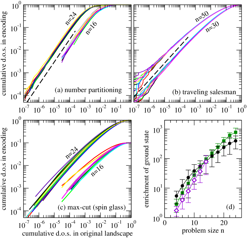
We now study enrichment as well as landscape structure on these three rather different problems. To this end, we consider the cumulative density of states

$$Q_{f}(\eta)=|\{x\in X:f(x)\leq\eta\}|\,/\,|X|$$ (4)

in the original landscape and $Q_{f\circ\alpha}$ defined analogously in the encoded landscape. In order to quantify the enrichment of good solutions, we compare the fraction $h$ of all states with an energy not larger than a certain threshold $\eta$ in the original landscape with the fraction $r(h)$ using the same threshold in the encoding. The encoding thus enriches low energy states if $r(h)\gg h$ for small $h$. Figure 1 shows that this is the case for the three landscapes and encodings considered here. We find in fact that the density of states $r(h)/h$ is enriched by several orders of magnitude in the encoded landscape, for all the cases considered.

Reassuringly, this trend of enrichment persists all the way to the ground state: that is, the encodings contain many more copies of the ground state than the original landscape. It appears in fact that the enrichment of ground states increases exponentially with system size. We can thus conclude that with the choice of an appropriately encoded landscape, it is easier both to find lower energy states from higher energy ones, and thus have more routes to travel to the ground state, as well as to reach the ground state itself from a low-energy neighbor, as a result of enrichment.

II.5 Neighborhoods and neutrality

Figure 2: Neutrality and encoded step length. (a) The fraction of neutral neighbors as a function of problem size. (b) The cumulative distribution of the distance moved in the original landscape by a single step in the encoding. Solid curves are for the max-cut, dashed curves for the number partitioning problem, with curve thickness distinguishing values of problem size $n$. For both plots (a) and (b), data have been obtained by uniform sampling of $10^{4}$ neighboring state pairs on $10^{2}$ independently generated instances of each type of landscape.

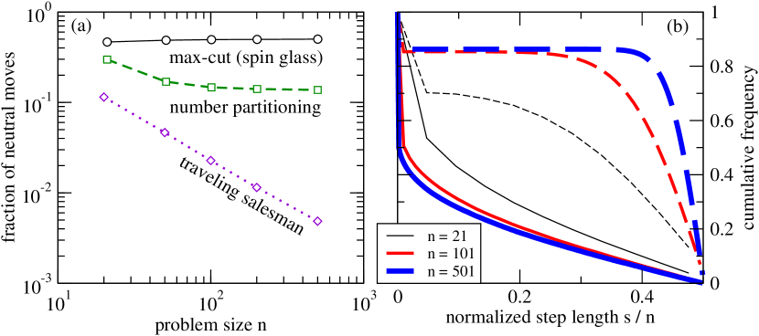
We continue the analysis of the encodings with attention to geometry and distances. A neutral mutation is a small change in the genotype that leaves the phenotype unaltered. In the present setting, a neutral move in the encoding is an edge $\{y,z\}\in M$ such that $\alpha(y)=\alpha(z)$. In general, the set of neutral moves is a subclass of all moves leaving the energy unchanged. An edge $\{x,y\}$ with $f(\alpha(x))=f(\alpha(y))$ but $\alpha(x)\neq\alpha(y)$ is not a neutral move in the present context. In the following, we examine the fraction of neutral moves for the encoded landscapes mentioned above.

Figure 2(a) shows that the fraction of neutral moves approaches a constant value when increasing the problem size of NPP and max-cut. The fraction of neutral moves in the traveling salesman problem, on the other hand, decreases as $1/n$ with problem size $n$. The average number of neighbors encoding the same solution grows linearly with $n$, since the total number of neighbors is $n(n-1)$ for each $y\in Y$ in the TSP encoding.

If a move in the encoding is non-neutral, how far does it take us on the original landscape? We define the step length of a move $\{y,z\}\in Y$ as the distance between the images of $y$ and $z$ on the original landscape,

$$s(\{y,z\})=d_{X}(\alpha(y),\alpha(z))$$ (5)

using the standard metric $d_{X}$ on the graph $(X,L)$. Obviously, $\{y,z\}$ is neutral if and only if $s(\{y,z\})=0$. Figure 2(b) compares the cumulative distributions of step length for number partitioning and max-cut. It is intractable to get the statistics of $s$ for the TSP problem for larger problem sizes since sorting by reversals, i.e., measuring distances w.r.t. to the natural move set, is a known NP-hard problem Caprara (1997).

For the encoding of number partitioning, step lengths are concentrated around $n/2$. Making a non-neutral move in this encoding is therefore akin to choosing a successor state at random. For the max-cut problem, the result is qualitatively different. Step lengths are broadly distributed with most moves spanning a short distance on the original landscape. Based on this it is tempting to conclude that optimization proceeds in ’smaller steps’ on the max-cut landscape, than in the NPP problem.

II.6 Evolutionary dynamics

Figure 3: Performance comparison between three types of stochastic dynamics: adaptive walks (AW) on the original ($\square$) and encoded ($\circ$) landscapes and randomly generate and test (RGT) on the encoded landscape ($\diamond$). The plotted performance value is the fraction of instances for which the considered evolutionary dynamics is “leading” at time $t$, i.e. has an energy not larger than the other two types of dynamics. For each landscape, 100 random instances are used with sizes $n=30$ in panels (a) and (b), $n=200$ in panel (c). On each of the instances, each type of evolutionary dynamics is run once with randomly drawn initial condition $y(0)\in Y$ for RGT and AW in the encoded landscape. The AW on the original landscape is initialized with the mapped state $x(0)=\alpha(y(0))$. Thus all three dynamics are started at the same energy.

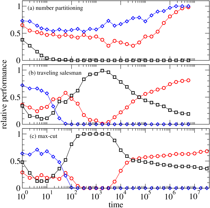
One might ask if the encoded landscape also facilitates the search dynamics, by virtue of its modified structure, and offers another avenue for optimization. For this purpose, we consider an optimization dynamics as a zero-temperature Markov chain $x(0),x(1),x(2),\dots$. At each time step $t$, a proposal $x^{\prime}$ is drawn at random. If $f(x^{\prime})\leq x(t)$, we set $x(t+1)=x^{\prime}$, otherwise $x(t+1)=x(t)$. This is an Adaptive Walk (AW) when the proposal $x^{\prime}$ is drawn from the neighborhood of $x(t)$. In Randomly Generate and Test (RGT), proposals are drawn from the whole set of configurations independently of the neighborhood structure. Thus a performance comparison between AW and RGT elucidates if the move set is suitably chosen for optimization. Because of the enrichment of low energy states by the encodings, it is clear that RGT performs strictly better on the encoding than on the original landscape.

Adaptive walks also perform strictly better on the encoding than on the original landscape, at least in the long-time limit, cf. Figure 3. Beyond this general benefit of the encodings, the dynamics shows marked differences across the three optimization problems. In the NPP problem, RGT outperforms AW on the encoded landscape, so that enrichment alone is responsible for the increase in optimization with respect to the original landscape. In the encodings of the other two problems, AW performs better than RGT so that we can conclude that the improved structure of the encoded landscape is also an important reason for the observed increase in performance, in addition to simple enrichment. The dynamics on the max-cut landscapes (panel c) has the same qualitative behavior as that on the TSP (panel a). Although there is a transient for intermediate times where adaptive walks on the original landscape seem to be winning, the asymptotic behavior is clear: adaptive walks on the encoded landscape perform best.

II.7 Conclusion

We have examined the role of encodings in arriving at optimal solutions to NP-complete problems: we have constructed encodings for three examples, viz. the NPP, Spin-Glass and TSP problems, and demonstrated that the choice of a good encoding can indeed help optimization. In the examples we have chosen, the benefits arise primarily as a result of the enrichment of low-energy solutions. A secondary effect in some but not all encodings considered here is the introduction of a high degree of neutrality. The latter enables a diffusion-like mode of search that can be much more efficient than the combination of fast hill-climbing and exponentially rare jumps from local optima. The two criteria, (1) selective enrichment of low energy states and, where possible, (2) increase of local degeneracy, can guide the construction of alternative encodings explicitly making use of a priori knowledge on the mathematical structure of optimization problem. The qualitative understanding of the effect of encodings on landscape structures in particular resolves apparently conflicting “design guidelines” for the construction of evolutionary algorithms.

The beneficial effects of enriching encodings immediately pose the question whether there is a generic way in which they can be constructed. The constructions for the NPP and TSP encodings suggest one rather general design principle. Suppose there is a natural way of decomposing a solution $x$ of the original problem into partial solutions. We can think of a partial solution $\xi$ as the set of all solutions that have a particular property. In the TSP example, $\xi$ refers to a set of solutions in which a certain list $A$ of cities appears as an uninterrupted interval. Now we choose the encoding $y$ so that it has an interpretation as a collection $\Xi(y)$ of partial solutions. A deterministic optimization heuristic can now be used to determine a good solution $x^{*}(\Xi(y))$. In the case of the TSP, $\Xi(y)$ corresponds to a set of constrained tours from which we choose by a greedy solution. Alternatively, $\Xi(y)$ may over-specify a solution, in which case the optimization procedure would attempt to extract an optimal subset of $\Xi^{\prime}\subseteq\Xi(y)$ so that $\bigcap_{\xi\in\Xi^{\prime}}\xi$ contains a valid solution $x^{*}$. In either case, $\alpha:y\mapsto x^{*}$ is an encoding that is likely to favour low-energy states. It is not obvious, however, that the spanning-tree encoding for max-cut can also be understood as a combination of partial solutions. It remains an important question for future research to derive necessary and sufficient conditions under which optimized combinations of partial solutions indeed guarantee that the encoding is enriching.

Methods

Landscapes and encoding

A finite discrete energy landscape $(X,L,f)$ consists of a finite set of configurations $X$ endowed with an adjacency structure $L$ and with a function $f:X\rightarrow\mathbb{R}$ called energy, and hence $-f$ fitness. The global minima of $f$ are called ground states. $L$ is a set of unordered tuples in $X$, thus $(X,L)$ is a simple undirected graph. Let $(Y,M)$ be another simple graph and consider a mapping $\alpha:Y\rightarrow X\cup\{\varnothing\}$, which we call an encoding of $X$. Then $(Y,M,f\circ\alpha)$ is again a landscape. (If we include states in $Y$ that do not encode feasible solutions we assign them infinite energy, i.e., $f\circ\alpha(y)=+\infty$ if $\alpha(y)=\varnothing$.) The encoding is complete if $\alpha$ is surjective, i.e., if every $x\in X$ is encoded by at least one vertex of $y\in Y$. Both landscapes then describe the same optimization problem. In the language of evolutionary computation, $(Y,M)$ is the genotype space, while $(X,L)$ is the phenotype space corresponding to the “direct encoding” of the problem. With this notation fixed, our problem reduces to understanding the differences between the genotypic landscape $(Y,M,f\circ\alpha)$ and the phenotypic landscape $(X,L,f)$ w.r.t. optimization dynamics.

Test Instances

Random instances fox max-cut (spin glass) are generated as standard random graphs Bollobas (2001) with parameter $p=0.5$: each potential edge is present or absent with equal probability, independent from other edges. Distances $d_{ij}=d_{ji}$ for the symmetric TSP and numbers $a_{i}$ for NPP are drawn independently from the uniform distribution on the interval $[0,1]$.

Enrichment factor and Density of States

The enrichment factor $r(h)$ can be obtained directly from the cumulative densities of states of the two landscapes:

$$r(h)=Q_{f\circ\alpha}(Q_{f}^{-1}(h))~{}.$$ (6)

This expression is a well-defined function for arguments $h\in[0,1]$ because $Q_{f\circ\alpha}$ only changes value where $Q_{f}$ also does. For ground state energy $\eta_{0}$, the enrichment of the ground state is $Q_{f\circ\alpha}(\eta_{0})/Q_{f}(\eta_{0})$.

The results in Figure 1(a-c) are obtained by sampling $2\times 10^{7}$ uniformly drawn states each from the original states $X$ and the prepartitionings $Y$ for the traveling salesman. For the two other problems, the density of states of the original landscapes is exact by complete enumeration. For the spin glass also, the density of states for $Y$ is exact from calculation based on the matrix-tree theorem. For number partitioning, $2^{n}$ samples in $Y$ are drawn at random.

The enrichment of the ground state, Figure 1(d), is an average over 100 realizations for each problem type and size $n$. For each realization of number partitioning and max-cut, $2^{n}$ uniform samples in $Y$ are taken; the ground state energy itself is obtained by complete enumeration of $X$. For each realization of the traveling salesman problem, $10^{9}$ uniform samples are taken in $Y$; the ground state energy is computed with the Karp-Held algorithm Held and Karp (1962).

References

- Garey and Johnson (1979) M. R. Garey and D. S. Johnson, Computers and Intractability. A Guide to the Theory of NP-Completeness (W. H. Freeman, 1979).
- Berg and Lässig (2004) J. Berg and M. Lässig, Proc. Nat. Acad. Sci 101, 14689 (2004).
- Fraenkel (1993) A. Fraenkel, Bull. Math. Biol. 55, 1199 (1993).
- Mézard and Zecchina (2002) G. Mézard, M. Parisi and R. Zecchina, Science 297, 812 (2002).
- Bauer and Orland (2005) M. Bauer and H. Orland, Phys. Rev. Lett. 95, 107202 (2005).
- Schulman (2007) L. S. Schulman, Phys. Rev. Lett. 9, 257202 (2007).
- Ricci-Tersenghi (2010) F. Ricci-Tersenghi, Science 330, 1639 (2010).
- Kirkpatrick et al. (1983) S. Kirkpatrick, C. D. Gelatt, and M. P. Vecchi, Science 220, 671 (1983).
- Holland (1992) J. H. Holland, Adaptation in Natural and Artificial Systems: An Introductory Analysis with Applications to Biology, Control, and Artificial Intelligence (The MIT Press, 1992).
- Koza (1992) J. R. Koza, Genetic Programming: On the Programming of Computers by Means of Natural Selection (The MIT Press, 1992).
- Reidys and Stadler (2002) C. M. Reidys and P. F. Stadler, SIAM Review 44, 3 (2002).
- Rothlauf and Goldberg (2003) F. Rothlauf and D. E. Goldberg, Evol. Comp. 11, 381 (2003).
- Rothlauf (2006) F. Rothlauf, Representations for Genetic and Evolutionary Algorithms (Springer, Heidelberg, 2006), 2nd ed.
- Applegate et al. (2006) D. L. Applegate, R. M. Bixby, V. Chvátal, and W. J. Cook, The Traveling Salesman Problem (Princeton Univ. Press, 2006).
- Flamm et al. (2007) C. Flamm, I. Hofacker, B. Stadler, and P. Stadler, LNCS 4436, 194 (2007).
- Schuster et al. (1994) P. Schuster, W. Fontana, P. F. Stadler, and I. L. Hofacker, Proc. Roy. Soc. Lond. B 255, 279 (1994).
- van Nimwegen and Crutchfield (2000) E. van Nimwegen and J. P. Crutchfield, Bull. Math. Biol. 62, 799 (2000).
- Choi and Moon (2008) S.-S. Choi and B.-R. Moon, IEEE Trans. Evol. Comp. 12, 604 (2008).
- Rothlauf (2011) F. Rothlauf, Design of Modern Heuristics: Principles and Application (Springer-Verlag, 2011).
- Fernández and Solé (2007) P. Fernández and R. V. Solé, J. R. Soc. Interface 4, 41 (2007).
- Yu and Miller (2002) T. Yu and J. F. Miller, Lect. Notes Comp. Sci. 2278, 13 (2002), euroGP 2002.
- Banzhaf and Leier (2006) W. Banzhaf and A. Leier, in Genetic Programming Theory and Practice III, edited by T. Yu, R. Riolo, and B. Worzel (Springer, New York, 2006), pp. 207–221.
- Knowles and Watson (2002) J. D. Knowles and R. A. Watson, LNCS 2439, 88 (2002).
- Reidys et al. (1997) C. Reidys, P. F. Stadler, and P. Schuster, Bull. Math. Biol. 59, 339 (1997).
- Mertens (1998) S. Mertens, Phys. Rev. Lett. 81, 4281 (1998).
- Ruml et al. (1996) W. Ruml, J. Ngo, J. Marks, and S. Shieber, J. Opt. Th. Appl. 89, 251 (1996).
- Karmakar and Karp (1982) N. Karmakar and R. M. Karp, Tech. Rep., UC Berkeley (1982), uCB/CSD 81/113.
- Sherrington and Kirkpatrick (1975) D. Sherrington and S. Kirkpatrick, Phys. Rev. Lett. 35, 1792 (1975).
- Binder and Young (1986) K. Binder and A. P. Young, Rev. Mod. Phys. 58, 801 (1986).
- Caprara (1997) A. Caprara, in Proceeding RECOMB ’97 (ACM, New York, 1997), pp. 75–83.
- Bollobas (2001) B. Bollobas, Random Graphs (Cambridge University Press, 2001).
- Held and Karp (1962) M. Held and R. M. Karp, J. Soc. Indust. and Appl. Math. 10, 196 (1962).