A Census of Star-Forming Galaxies at $z=1$–3 in the Subaru Deep Field

Abstract

Several UV and near-infrared color selection methods have identified galaxies at $z=1$–3. Since each method suffers from selection biases, we have applied three leading techniques (Lyman break, BX/BM, and BzK selection) simultaneously in the Subaru Deep Field. This field has reliable ($\Delta z/(1+z)=0.02$–0.09) photometric redshifts for $\sim$53,000 galaxies from 20 bands (1500 Å–2.2 $\mu$m). The BzK, LBG, and BX/BM samples suffer contamination from $z<1$ interlopers of 6%, 8%, and 20%, respectively. Around the redshifts where it is most sensitive ($z\sim 1.9$ for star-forming BzK, $z\sim 1.8$ for $z\sim 2$ LBGs, $z\sim 1.6$ for BM, and $z\sim 2.3$ for BX), each technique finds 60%–80% of the census of the three methods. In addition, each of the color techniques shares 75%–96% of its galaxies with another method, which is consistent with previous studies that adopt identical criteria on magnitudes and colors. Combining the three samples gives a comprehensive census that includes $\approx$90% of $z_{\rm phot}=1$–3 galaxies, using standard magnitude limits similar to previous studies. In fact, we find that among $z=1$–2.5 galaxies in the color selection census, 81%–90% of them can be selected by just combining the BzK selection with one of the UV techniques ($z\sim 2$ LBG or BX and BM). The average galaxy stellar mass, reddening, and star formation rates (SFRs) all decrease systematically from the sBzK population to the LBGs, and to the BX/BMs. The combined color selections yield a total cosmic SFR density of 0.18$\pm$0.03 $M_{\sun}$ yr^-1 Mpc^-3 for $K_{\rm AB}\lesssim 24$. We find that 65% of the star formation is in galaxies with $E(B-V)>0.25$ mag, even though they are only one-fourth of the census by number.

1. INTRODUCTION

Several color techniques have succeeded in identifying large samples (thousands) of galaxies in various windows of high redshift. They work by using deep wide-field imaging in only a few broad-band filters. In the simplest cases, only two colors are needed to isolate a spectral break. For imaging surveys limited to optical observations, the Balmer/4000 Å break is measurable up to $z\approx 1$, and the Lyman continuum break is detectable starting at redshifts of 3 and higher (e.g., Steidel et al., 1999; Bouwens et al., 2006; Yoshida et al., 2006). But at intermediate redshifts, CCDs are only sensitive to the spectral region between these two strong features. The resulting inability to identify galaxies at $z\approx 1$–3, has lead to this range being called the “redshift desert.” Finding large samples of galaxies in the redshift desert requires detections of the Balmer break with near-infrared photometry, or the Lyman break with ultraviolet imaging.

The extension of the Lyman break technique to $z<2.6$ requires deep near-ultraviolet (NUV) imaging, which has only been recently available with the GALEX satellite (Ly et al., 2009, hereafter L09) and Hubble WFC3/UVIS (Hathi et al., 2010). Prior to this, different techniques were developed, to select “BX” and “BM” galaxies (Adelberger et al., 2004; Steidel et al., 2004), BzK galaxies (Daddi et al., 2004), and “distant red galaxies” (DRGs; Franx et al., 2003; van Dokkum et al., 2004). However, each technique suffers from its own selection biases. For example, UV selections (e.g., LBG, BX) tend to identify young star-forming galaxies with low dust extinction, while IR techniques (e.g., BzK, DRG) select more massive, dusty galaxies.

In this paper, we apply several color selection techniques to our panchromatic photometry of the Subaru Deep Field (SDF), to identify $\approx$21,000 galaxies at $z=1$–3 for a census of optical and near-infrared (NIR) selected star-forming galaxies. Throughout this manuscript, the term “census” will be repeatedly use to refer to the union of the different color selection methods that identify LBGs, BX/BMs, and sBzK galaxies down to specific magnitude depths that are typical of past and current $z\sim 2$ census studies. Our multi-technique survey, compared to previous work (Reddy et al., 2005; Quadri et al., 2007; Grazian et al., 2007, hereafter R05, Q07, and G07, respectively), has significantly more galaxies because our deep imaging covers 2–10 times more area. Since we also have a wide range of photometry spanning many filters, we can then directly compare these simple color techniques to a sample derived from photometric redshift (Baum, 1962, hereafter photo-$z$ or $z_{\rm phot}$).

Table 1Summary of SDF Multi-wavelength Data

Filter	$\lambda_{\rm cen}$	$\lambda_{\rm FWHM}$	FWHM (″)	$m_{\rm lim}^{\rm AP}$	Ap. Corr.	$m_{\rm lim}^{\rm TOT}$	$N$($3\sigma$)	$N$($5\sigma$)
$FUV$	string1533	string209	$\sim$4.5	26.286	1.454	25.880	13895 string(16859)	string6592 string(8016)
$NUV$	string2284	string697	$\sim$5.0	26.596	1.845	25.931	47845 string(57668)	30271 (36470)
$U$	string3634	string750	1.49	26.287	1.164	26.122	34926 string(42379)	24124 (29257)
$B$	string4438	string687	1.01	28.066	1.192	27.876	88703 (107935)	74836 (91017)
$V$	string5463	string885	1.11	27.338	1.178	27.161	75522 string(92182)	62341 (76025)
$R_{\rm C}$	string6515	string1100	1.11	27.528	1.173	27.355	90452 (110151)	76773 (93466)
$i$′	string7659	string1419	1.11	27.202	1.168	27.034	82308 (100245)	69666 (84902)
$z$′	string9020	string956	0.96	26.270	1.181	26.090	57163 string(69778)	46767 (57017)
$z_{b}$	string8842	string620	0.91	25.806	1.175	25.631	47067 string(57551)	36289 (44405)
$z_{r}$	string9841	string1000	0.91	24.946	1.274	24.683	28989 string(35276)	21853 (26571)
$IA598$	string6007	string303	0.91	26.276	1.262	26.023	47764 string(58322)	34987 (42724)
$IA679$	string6780	string340	0.96	26.870	1.214	26.659	72221 string(87969)	57672 (70361)
$J$	12492	string1799	1.27	22.894	1.214	22.684	16694 string(19985)	string9637 (11713)
$H$	16186	string5700	1.18	22.328	1.208	22.123	10662 string(12691)	string5684 string(6949)
$K$	22035	string2995	0.81	23.673	1.172	23.500	24788	17415
NB704	string7046	string100	0.91	26.112	1.150	25.960	52193 string(63537)	39438 (47951)
NB711	string7111	string72	0.91	25.533	1.206	25.330	36893 string(44871)	25580 (31205)
NB816	string8150	string120	0.91	26.404	1.142	26.259	66728 string(81313)	52492 (63960)
NB921	string9196	string132	0.96	26.045	1.167	25.878	57461 string(70347)	44847 (54809)
NB973	string9755	string200	0.91	25.086	1.255	24.840	37001 string(44990)	26350 (32067)
$[3.6]$ 2″ $\phi$	35634	string7500	…	24.433	1.059	24.371	92534 (104282)	87628 (97728)
$[3.6]$ 4″ $\phi$	…	…	2.25	23.192	1.424	22.809	90411 (101482)	83352 (92057)
$[4.5]$ 2″ $\phi$	45110	10000	…	24.014	1.230	23.790	87228 string(97890)	81200 (89907)
$[4.5]$ 4″ $\phi$	…	…	2.10	22.817	1.456	22.409	81915 string(90890)	75896 (82998)

The observations spanning wavelengths from 1500 Å to 4.5 µm and their reductions are described in Section 2. Section 3 describes the merging of the multi-wavelength data together, which accounts for differences in the spatial resolution across different wave bands. Section 4 discusses the determination of photo-$z$ and the modeling of the spectral energy distribution (SED). In Section 5, the different color selection techniques used and individual sample properties are presented. Section 6 discusses the selection effects of one technique against another, and compares them with our $z_{\rm phot}$-selected sample. We also compare our results with previous surveys. In Section 7, we present a Monte Carlo simulation that aims to generate a mock census of $z\approx 1$–3 galaxies to support many of our observed relations and results. Conclusions from our $z=1$–3 census survey are summarized in Section 8.

Throughout this paper, a flat cosmology with [$\Omega_{\Lambda}$, $\Omega_{M}$, $h_{70}$] = [0.7, 0.3, 1.0] is adopted. Magnitudes are reported on the AB system (Oke, 1974), and unless otherwise indicated, limiting magnitudes are 5$\sigma$, corrected for the flux falling outside of the apertures assuming an unresolved source (i.e., total limiting magnitudes). Diameter apertures sizes are denoted with a “$\phi$.”

2. Subaru Deep Field Multi-Wavelength Observations

A summary of the depth, spatial resolution, and sample sizes for the imaging data is provided in Table 1, while the spatial coverage of the SDF at different wavebands is shown in Figure 1. Although the reported depths illustrate the sensitivity of the data, we emphasize that all of the sources actually analyzed later in this paper are detected well above these $5\sigma$ limits in almost all of the wavebands. The only exceptions are the FUV, NUV, $J$, $H$, and $K$ bands. Since most of these data are described in previous papers, only brief summaries are presented.

2.1. Subaru/Suprime-Cam Data

The $BVR_{\rm C}i\arcmin z\arcmin$ observations are the deepest data obtained to date from Suprime-Cam (Miyazaki et al., 2002), and are described in Kashikawa et al. (2004). The total limiting magnitudes were redetermined with more rigorous masking of pixels affected by object flux and are $\approx 0.1$–0.2 mag deeper than those quoted in Ly et al. (2007). They range from 26.1 to 27.9 mag.

In addition to these data, Suprime-Cam imaging in four intermediate-band filters, IA598, IA679, $z_{b}$, and $z_{r}$ are also available. Studies (e.g., Meisenheimer & Wolf, 2002; Ilbert et al., 2009; van Dokkum et al., 2009) using intermediate-band filters have improved photo-$z$ estimates, as they are able to identify the location of spectral breaks more accurately. The $z_{b}$ and $z_{r}$ observations were obtained in 2003 and 2004, and are described in Shimasaku et al. (2005). The net integration times are 85 and 600 minutes for $z_{b}$ and $z_{r}$, which give total limiting magnitudes of 25.6 and 24.7 mag, respectively. The IA598 and IA679 observations were obtained in 2007 and are described in Nagao et al. (2008). Their depths are 26.0 and 26.7 mag, respectively.

Finally, we include imaging in five narrow-band (NB) filters (NB704, NB711, NB816, NB921, and NB973). These data are included to specifically help improve the $z_{\rm phot}$’s for emission-line galaxies, but we find redshift accuracy improvements for galaxies at $z\lesssim 1.6$. Their 5$\sigma$ total flux depths vary between 24.9 and 26.2 mag. The narrow-band data reduction is further discussed in Ouchi et al. (2003), Shimasaku et al. (2003), Shimasaku et al. (2004), and Kashikawa et al. (2004).

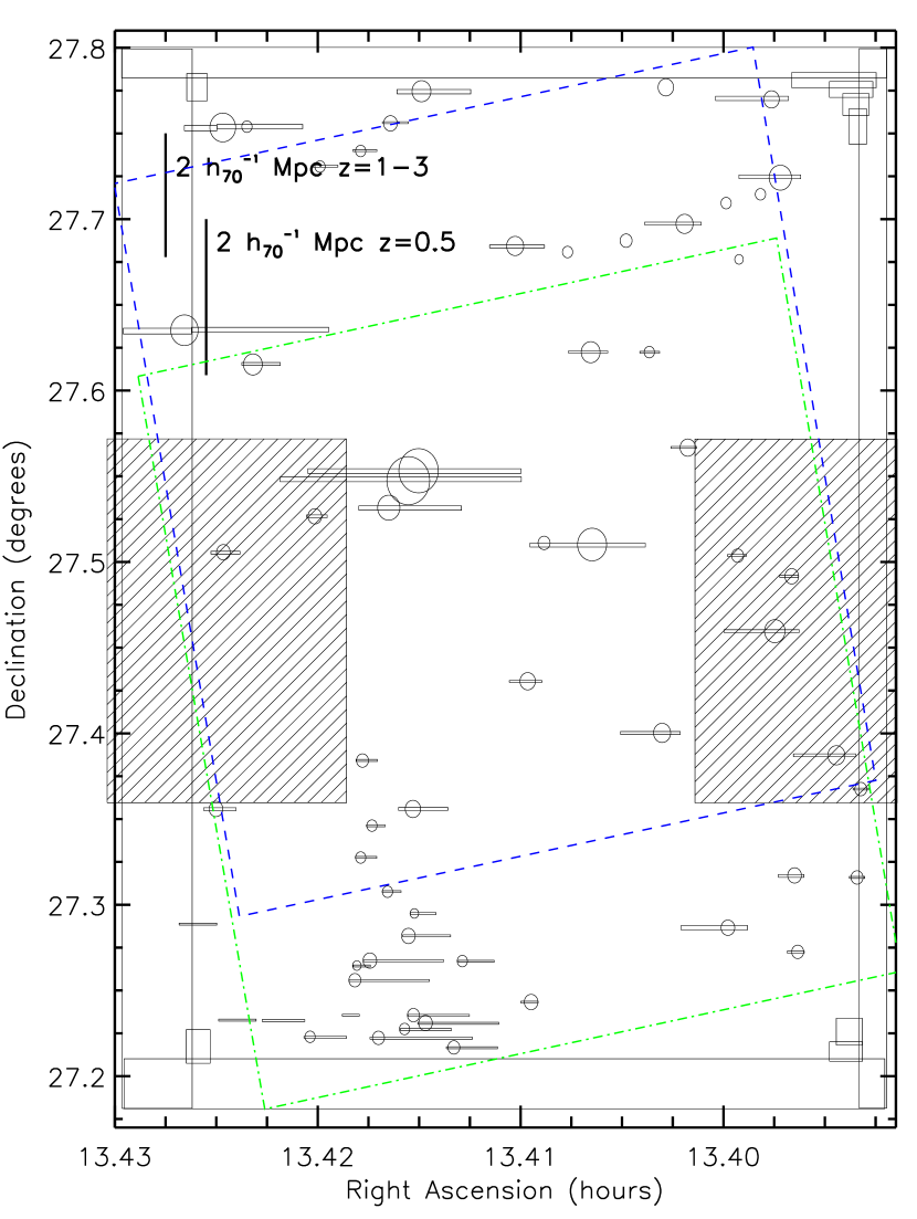
Figure 1.— Sky coverage of SDF data described in Section 2. Masked regions for the Suprime-Cam data are shown with the solid black rectangles and circles. Excluding these regions, the area coverage is 870.4 arcmin². The shaded regions correspond to lower $K$-band sensitivity areas (718.7 arcmin² has deep $K$ coverage). GALEX, NEWFIRM, and MOSAIC data have coverage over the entire SDF. Spitzer 1 ks IRAC coverage is illustrated with the dashed line (blue; [3.6] and [5.8]) and dot-dashed line (green; [4.5] and [8.0]). The angular size for 2 h${}_{70}^{-1}$ Mpc is shown by the thick bars for $z=0.5$ and $z=1$–3. (A color version of this figure is available in the online journal.)

2.2. UKIRT/WFCAM Data

$K$-band data for this survey were acquired with Wide-Field Camera (WFCAM; Casali et al., 2007) on the United Kingdom Infrared Telescope (UKIRT) on 2005 April 14–15 and 2007 March 5–6. Because the field of view (FoV) of WFCAM is split into four 13$\farcm$6$\times$13$\farcm$6 images separated by 12$\farcm$8, four pointings were required to cover the whole SDF optical image. The total exposure time for each pointing is 294–300 minutes, except for one pointing of 15 minutes. We ignore the less sensitive regions, so 80% of the SDF optical coverage has uniform $K$-band data down to the deepest sensitivity (see Figure 1). Previous results using a subset of this data were presented in Hayashi et al. (2007). The data were reduced following standard NIR reduction procedures in IRAF. Photometric and astrometric calibrations were carried out against Two Micron All Sky Survey (2MASS; Skrutskie et al., 2006) stars. The final $K$-band data reach a total $5\sigma$ depth of 23.5 mag.

2.3. Mayall/MOSAIC Data

$U$-band data were obtained from the KPNO Mayall 4 meter telescope with the Mosaic-1 Imager (FoV of 36′; Muller et al., 1998) on 2007 Apr 18 and 19. Observing conditions were dark with minimal cloud coverage. A series of 25 minute exposures was obtained to accumulate 47 ks for a 5$\sigma$ total depth of 26.1 mag. A standard dithering pattern was followed to provide more uniform imaging across the $\approx$10″ CCD gaps. The MSCRED IRAF (version 2.12.2) package was used to reduce the data and produced final mosaic images with a pixel scale of 0$\farcs$258 and an average-weighted seeing of $\approx$1$\farcs$5 FWHM. The reduction steps followed closely the procedures outlined for the reduction of the MOSAIC data for the NOAO Deep Wide-Field Survey.

While several Landolt (1992) standard star fields were observed, Landolt’s $U$ filter differs significantly from the MOSAIC/$U$, which makes it difficult to calibrate the photometry. One hundred and two Sloan Digital Sky Survey (SDSS) stars distributed uniformly across the eight Mosaic-1 CCDs with $u\arcmin\lesssim 21$ mag were used. This approach requires a transformation between SDSS $u$′ and MOSAIC/$U$, which is obtained by convolving the spectra of 175 Gunn–Stryker stars with the total system throughput at these wavebands. These stars span $B-V=-0.2$–0.8 mag, and show that the $B-V$ color term is smaller than the scatter (1$\sigma$ = 0.06 mag) in the predicted U magnitudes.

2.4. GALEX/NUV and FUV Data

The GALEX space telescope (Martin et al., 2005) provides simultaneous $FUV$ and $NUV$ imaging with a pixel scale of 1$\farcs$5 and an FoV of 1$\fdg$2, thus covering the entire SDF. A total of 161225 s (80851 s) was obtained in the $NUV$ ($FUV$) band (Malkan, 2004). The data were processed through the GALEX reduction pipeline and stacked accordingly. The FWHM of unresolved images is 4$\farcs$5 in the $FUV$ and 5$\farcs$0 in the $NUV$. The 5$\sigma$ total limiting magnitudes are both $\approx$25.9 mag.

2.5. Mayall/NEWFIRM Data

$J$- and $H$-band observations were obtained from the NOAO Extremely Wide-field Infrared Imager (NEWFIRM; Probst et al., 2004, 2008) on 2008 May 10–12. Exposures of 60 ($J$) and 20 or 30 ($H$) s were taken with a simple five-point dithering pattern to image across the detector gaps ($\approx 35\arcsec$ in size) and to avoid latent images of bright sources on the same source. A total of 27.5 ks and 5.5ks were acquired in $J$ and $H$, respectively. While cloud coverage was minimal, the conditions were non-photometric (e.g., the effective $J$ exposure time was approximately 9ks). These NEWFIRM data required a first-pass reduction to create a deep object mask. This mask is then used to create flat-fields and sky images to enable proper subtraction of the sky background. Then the sky-subtracted images were used for the second-pass processing to create the final mosaics. The $J$ ($H$) limiting magnitude was determined to be 23.4 (22.8) mag in a 3″ $\phi$ aperture, and the average seeing is $\approx$1$\farcs$3 (1$\farcs$2).

2.6. Spitzer/IRAC Data

Imaging in the IRAC bands was conducted in 2006 February 11 and 14 (Prop#20229; Malkan et al., 2005). The observations consisted of nearly uniform coverage in all four bands of 1 ks. The coverage is $26\arcmin\times 25\farcm 5$ for [3.6] and [5.8] or [4.5] and [8.0], and the overlapping region for all four bands is approximately $19\arcmin\times 25\farcm 5$. Version S13.2 data products were used. Necessary pre-processing steps were taken to remove detector artifacts (e.g., mux-bleeding, column pull-downs) with contributed software provided by the IRAC community, and the data reduction followed standard procedures using the MOsaicker and Point source EXtractor (MOPEX) package. The astrometric solutions for the mosaics were examined against 2MASS stars and are accurate to with 0$\farcs$1.

Apertures were placed randomly on the images to determine the limiting depth. The depths are summarized in Table 1. For the remainder of this paper, we only use the [3.6] and [4.5] data, since they sample rest frame $\sim 1$–2 $\mu$m for $z=1$–3, which are unaffected by polycyclic aromatic hydrocarbon (PAH) features.

The greatest limitation of the IRAC data is the spatial resolution: measuring unresolved galaxies generally requires at least a 4″ $\phi$ aperture. Recently, Velusamy et al. (2008) developed a high-resolution image deconvolution code (HiRes) to handle Spitzer data. The code has been found to significantly improve the quality of the images, allowing for smaller photometric apertures and a reduction of source confusion. HiRes was used on these IRAC data, and the results show improvements in the aperture fluxes by a factor of 2–4 using the same aperture sizes. For example, a 2″ $\phi$ aperture was able to encompass 95% and 81% of the total light in [3.6] and [4.5], respectively. We examined sources in both images and found that photometric fluxes are conserved, indicating that these HiRes images can be used to attain reliable flux measurements in these bands. This improvement allowed for the crucial detection of lower mass galaxies at $z\sim 2$ at rest 1 $\mu$m.

3. The SDF Multi-band Galaxy Sample

3.1. Synthesizing Multi-band Data

Methodology. A key requirement of this survey is to merge the full SDF multi-wavelength data. However, the spatial resolution varies by a factor of a few for the different instruments. Simply degrading the best data ($\sim$1″) to match the poorest resolution (4″–5″ for GALEX data) will hamper the identification of faint galaxies, most of which are at high redshift.

A solution to this problem is a hybrid approach of (1) slightly degrading high-resolution images to match a “baseline” spatial resolution that is not significantly different and (2) using aperture corrections. This method will not greatly compromise sensitivity, and the aperture corrections are reliable, since this work mostly probes compact galaxies (they are faint and at high-$z$).

We begin by combining multiple broad- and intermediate-band images into a single ultra-deep frame. This approach benefits from the inclusion of weak sources that are marginally detected in individual wave bands, but are highly significant in the merged image. This ultra-deep image serves as a reference image when running SExtractor (Bertin & Arnouts, 1996) in “dual image” mode. It yields a catalog of sources in the SDF, and later serves as the “master object list” for the photo-$z$ catalogs and the color-selected samples. The similarities of the spatial resolution for $BVR_{\rm C}i\arcmin z\arcmin K$, IA598, and IA679 allow us to degrade these images to a 1$\farcs$1 (hereafter “psf-matched”). The inclusion of $K$ implies that this ultra-deep mosaic is simultaneously sensitive to optically selected and NIR-selected galaxies.

To stack these images, we use the $\chi^{2}$-weighting scheme of Szalay et al. (1999). This method uses the $\chi^{2}$ of each pixel, imaged in $N$ bands, to estimate the probability that it is sampling a source or the sky. First, for image $i$, the mean ($\mu_{i}$) is removed, and then the image is scaled by the sky rms fluctuation ($\sigma_{i}$):

$$g_{i}(x,y)=\frac{f_{i}(x,y)-\mu_{i}}{\sigma_{i}},$$ (1)

where $f_{i}(x,y)$ is the measurement (in count rates, electrons, or fluxes) in image $i$, and $g_{i}(x,y)$ can be viewed as the signal-to-noise ratio (S/N) for a given pixel. Then, we sum the squares of these 8 S/N images to yield the ultra-deep image: $y=\displaystyle\sum_{i=1}^{8}g_{i}^{2}$.

We considered including additional wave bands into the ultra-deep image, but they degraded the results due to their lower sensitivities and/or poorer spatial resolutions. For example, the $U$-, $J$-, and $H$-band data have lower spatial resolution ($\sim 1\farcs 5$) and are less sensitive than the nearby $B$- and $K$-band data. Similarly, including the narrow-band observations does not increase the sample sizes. These data are shallower than the broad-band SDF observations, so almost all of the narrow-band selected sources are identified in the broad-band images. While there are some galaxies that are only detected in the narrow-band observations and thus missed by our multi-band $\chi^{2}$ image (e.g., Ly$\alpha$ emitting galaxies at $z\gtrsim 5$), this tiny galaxy population is less than 0.05% of the full catalog, and will not affect the $z=1$–3 galaxy census that we later derive. For these Ly$\alpha$ emitters, it is better to generate a separate sample using only the narrow-band observations, as done in Kashikawa et al. (2006) and Shimasaku et al. (2006), for example.

Source catalogs. We run SExtractor on the square root of the ultra-deep $\chi^{2}$ image to obtain a total of 243,964 sources with a minimum of five connected pixels above a $\chi=3.5$ threshold, of which 211,594 sources are in the unmasked regions shown in Figure 1. This sample is further reduced to 174,837 sources when the poorly sampled $K$-band regions are excluded. This is the largest photometric catalog for the SDF.

One concern with the multi-band catalog is that it may systemically miss some galaxies, particularly the bluest and reddest ones, because they are undetected in the longer or shorter bandpasses, respectively. We investigate this possibility by generating $BVR_{\rm C}$ and $i\arcmin z\arcmin K$ stacked mosaics using the $\chi^{2}$ weighting approach. We run SExtractor on these stacked images, and compare these catalogs against the ultra-deep eight-band catalog. First, we find that the overlap is $\approx$90% or larger at any given magnitude in any of the individual bands. Second, since galaxies with extreme colors could be systematically missed, we also examine the overlap of the bluest (reddest) quartile of $BVR_{\rm C}$ ($i\arcmin z\arcmin K$) catalog against our eight-band catalog. The blue sample consists of $\sim$20,000 galaxies with $B-V<0.2$ mag while the red sample contains $\sim$6000 galaxies with $z\arcmin-K>0.4$ mag. Fortunately, the overwhelming majority of these galaxies with extreme colors were already included in the original selection using the eight-band ultra-deep image, 93% and 89% of the blue and red samples, respectively. We find that these fractions hold regardless of magnitudes or colors. These tests and comparisons indicate that the multi-band synthesis approach does not inherently miss any significant population of galaxies. We will discuss this issue further in Section 7. Szalay et al. (1999) also find that the approach is optimal when generating source catalogs for the Hubble Deep Field.

Measured fluxes. Generally, fluxes are measured in fixed circular apertures with diameter sizes comparable to twice the FWHM of resolution, and are then corrected for aperture losses, which are listed in Table 1. Thus, for images with $\lesssim 1\arcsec$, we measure photometric fluxes in 2″ $\phi$ aperture with SExtractor. For the $U$, $J$, and $H$ bands, we use 3″ $\phi$ aperture measurements. The GALEX and IRAC/HiRes bands use a 6$\farcs$8 and 2″ $\phi$ apertures, respectively. For the GALEX and IRAC/HiRes data, the images were not matched to the Suprime-Cam pixel scale. Instead, we use DAOPHOT to measure the fluxes at known positions, which follows the identical procedure discussed in L09. One advantage of DAOPHOT is that additional noise is not introduced when these images are regridded to the reference SDF Suprime-Cam image with a pixel scale of 0$\farcs$2.

GALEX source confusion. One concern for GALEX FUV and NUV measurements is source confusion—the overestimation of the flux for faint sources that happen to fall in the wings of brighter nearby sources. To correct for this, we take a point-spread function (PSF)-fitting approach, which supersedes the baseline approach of fixed aperture measurements. This consists of two stages: (1) fitting and removing relatively bright sources with an empirical PSF constructed from a dozen unresolved bright sources, and (2) then for fainter sources, aperture photometry can be done on the image with the relatively bright sources removed. The GALEX fluxes for the bright and faint sources are then combined together for a single catalog.

The PSF fitting is done using a few DAOPHOT tools. DAOPHOT assumes that sources are unresolved relative to the PSF. Since 97% (51%) of the objects in our multi-band source catalogs are 3″ (1$\farcs$1) FWHM or smaller, the large spatial resolution of 4″–5″ for GALEX implies that modeling and removing sources with a point-like PSF is a valid approach for almost all sources.

Prior inputs to fitting the GALEX observations are based on detections in the $U$ band. A total of 43,839 (31,084) sources were considered for NUV (FUV) PSF fitting down to 26.75 mag (for NUV) and 26.25 mag (for FUV), which is much deeper than any previous photometric studies with GALEX. Only 18,036 (14,341) sources were actually PSF-fitted, since the remaining sources were either too faint or too close to another brighter object.

While PSF fitting is done for bright sources, we still determine the total fluxes using the fixed aperture flux measurements and apply aperture corrections. This ensures that all fluxes are obtained in a consistent manner. We note that we compare “total” flux measurements with those obtained from PSF-fitting for bright sources, and find them to be consistent within the uncertainties. This is expected, since the aperture corrections are derived from the empirical PSF, which is used to fit and remove the flux from the wings of sources. One form of “quality assurance” is to compare the “noise” in the original GALEX image to that of the “cleaned” image, after PSF-fitting subtraction. Visual inspection shows that the source-subtracted image looks very much like pure white sky noise. We quantified this by measuring the 1$\sigma$ fluctuations in the same area with same clipping algorithm, and find that the rms is reduced by 50% after the sources are PSF-fitted and removed. In fact, the rms of the cleaned NUV image, 19 photons per pixel, is only slightly larger than the predicted rms based on Poisson count statistics ($\sim 16$). Similarly, the cleaned FUV image has an average sky background of 13 photons per pixel. The square root of this is 3.6 photons, which is very close to our observed rms fluctuations of 3.9 photons. Thus the sky noise in our cleaned picture is nearly as small as the limit set by the photon statistics of the sky background.

3.2. The Identification of Stars

To identify foreground stars we use two techniques. First, stars can be easily identified in the NIR, since it measures the Rayleigh–Jeans tail, and forms a stellar locus in color space distinct from galaxies. Studies that have selected BzK galaxies also distinguished stars by their $z\arcmin-K$ colors (see e.g., Q07, ). For sources detected in the $K$ band, we classify 1603 stars with $z\arcmin-K\leq 0.455(B-z\arcmin)-0.773$ and $z\arcmin-K\leq 0.235(B-z\arcmin)-0.279$.

For sources that are undetected in $K$ (or lack $K$ data), we use the technique (called the $\Delta$ method) that is described in L09. First, objects were considered potential stellar candidates based on how similar they are to the PSF. They were assigned a number between 0 and 10 (10 being most PSF-like). However, unresolved galaxies might also be very compact. Therefore, to distinguish these galaxies from stars, we then calculate their deviation from the stellar locus in the $B-V$, $V-R_{\rm C}$, and $R_{\rm C}-z\arcmin$ colors. This deviation ($\Delta$) from the locus in a multi-color space is certainly affected by photometric scatter for faint sources, so we limit stellar identification with the $\Delta$ method to $V=25.0$. $\Delta$ values for $\sim$67,000 sources are illustrated in Figure 2, and show a strong peak at $\Delta\approx 0$ (the secondary peak is for low-$z$ galaxies).

One of the best tests of this method is to compare with the sample identified from $B-z\arcmin$ and $z\arcmin-K$ colors. The distribution of $\Delta$ for the 1603 $K$-band selected stars is plotted in Figure 2 and supports the $\Delta$ method. Among the $K$-band stellar sources, 82% (1315/1603) of them have point-like rank values of 4 and higher. Thus, we classify undetected $K$-band sources with rank values of at least 4, $V<25.0$, and $\Delta$ values within $3\sigma$ of the expected fluctuations in $\Delta$-magnitude relation as stellar sources. This yielded 1167 additional sources, for a total of 2770 stellar sources. We removed these stellar sources from our full catalog and report stellar contamination for individual galaxy selection samples below.

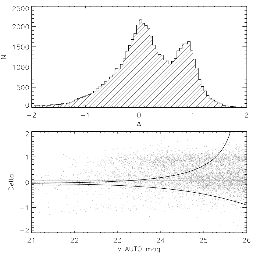
Figure 2.— Deviation ($\Delta$) in magnitudes from the stellar locus in a three-color space. (Left) Distribution of $\Delta$ is shown for $\sim$67,000 sources with point-like rank of 4–10 in the top panel and against $V$ in the bottom panel. The solid lines correspond to a minimum $\Delta=\pm 0.1$ mag and the $\pm 3\sigma$ fluctuations expected from a combination of the $B$, $V$, $R_{\rm C}$, and $z\arcmin$ depth. (Right) The distribution of $\Delta$ for $K$-band selected stellar sources based on their $B-z\arcmin$ and $z\arcmin-K$ colors. This shows that the majority of stellar sources have $\Delta\approx 0$.

4. Photometric Redshifts and SED Modeling

4.1. Photometric Redshifts

For this survey, the number of spectroscopic redshifts is limited ($N\sim 1000$), so well calibrated $z_{\rm phot}$’s are used. These $z_{\rm phot}$’s are determined from 20 bands (FUV, NUV, $UBVR_{\rm C}i\arcmin z\arcmin z_{b}z_{r}JHK$, IA598, IA679, and five narrow-band filters) using the Easy and Accurate $z_{\rm phot}$ from Yale (EAZY; Brammer et al., 2008) package. This photo-$z$ code has the following advantages: (1) it is easy to use and fast, (2) it handles input measurements in fluxes rather than magnitudes (e.g., hyperz; Bolzonella et al., 2000), which is crucial for non-detections (see below), and (3) it has been well calibrated against existing optical-to-NIR data with spectra for $\sigma_{z}/(1+z)\approx 0.03$.

Throughout the paper, redshift distribution is described by N($z$), which uses the peak of the probability redshift distribution. We have compared N($z$) for a subset of galaxies at high redshift to the distribution made by adding the full redshift distribution for each galaxy. We find that the two distributions are in agreement, justifying the use of the peak.

Illustrated in Figure 3 is a comparison of photometric and spectroscopic redshifts for 495 sources using 20 bands. The spectroscopy was obtained from Subaru, MMT, and Keck. The inclusion of the NUV improved photo-$z$ accuracy by $\approx$17% compared to $UBVR_{\rm C}i\arcmin z\arcmin z_{b}z_{r}JK$, IA598, and IA679 alone. $H$ and FUV measurements added a further $\sim$10% improvement. Photo-$z$’s derived from 15 bands (excluding narrow-bands) are accurate to 2.5% out to $z\approx 1.8$, and $\approx$1.2% by including the narrow-band measurements. Spitzer/IRAC measurements were also included, but produced little improvement. In particular, we found more problems at lower redshift, and this is likely due to PAH features that have not been included in the photo-$z$ templates. We find that the catastrophic failure rate is $\sim$10%. A preliminary examination indicates that one-fourth of these failures are due to galaxies with very strong optical emission lines.

Our photometric redshifts of galaxies with emission lines identified with narrow-band filters (see Ly et al., 2007) are also found to be reliable. Among 5029 narrow-band excess line emitters between $z=0.24$ and $z=1.47$, 4568 have $z_{\rm phot}$ estimates. This is almost 10 times the number of spectra that we used to compare $z_{\rm phot}$ with $z_{\rm spec}$. We estimate the median $z_{\rm phot}$ and find good to reasonable agreement prior to including narrow-band measurements and additional improvement with the narrow-band filters included (see Table 2).

Table 2Photometric Redshifts for Emission-line Galaxies

Sample	$z_{\rm NB}$	$z_{\rm phot}$(15-band)	$z_{\rm phot}$(20-band)
H$\alpha$ NB816	0.243	0.257$\pm$0.015	0.233$\pm$0.003
H$\alpha$ NB921	0.401	0.410$\pm$0.008	0.396$\pm$0.007
[O III] NB704	0.407	0.409$\pm$0.007	0.403$\pm$0.000
[O III] NB711	0.423	0.428$\pm$0.004	0.431$\pm$0.000
[O III] NB816	0.630	0.635$\pm$0.009	0.645$\pm$0.046
[O III] NB921	0.837	0.788$\pm$0.010	0.835$\pm$0.000
[O II] NB704	0.891	0.797$\pm$0.088	0.890$\pm$0.000
[O II] NB711	0.912	0.890$\pm$0.013	0.909$\pm$0.000
[O II] NB816	1.189	1.093$\pm$0.272	1.193$\pm$0.002
[O II] NB921	1.467	1.537$\pm$0.033	1.473$\pm$0.000

These $z_{\rm phot}$’s derived without the inclusion of narrow-band data confirm (1) the ability of Ly et al. (2007) to distinguish H$\alpha$, [O III], and [O II] emitters accurately using simple two-color selection, and that (2) the $z_{\rm phot}$ derived for SDF galaxies are reliable.

Figure 3.— Comparison of photometric and spectroscopic redshifts. A total of 495 spectroscopic sources have $z_{\rm phot}$ estimates. The $z_{\rm phot}$ are derived from 20-band photometry and show accuracy of $(z_{\rm phot}-z_{\rm spec})/(1+z_{\rm spec})\approx 0.012$ with less than 1% systematic offset. We find similar results using a smaller sample that has $>5\sigma$ detection in K. Solid lines are shown for $\pm$5%, $\pm$10%, and $\pm$20% errors.

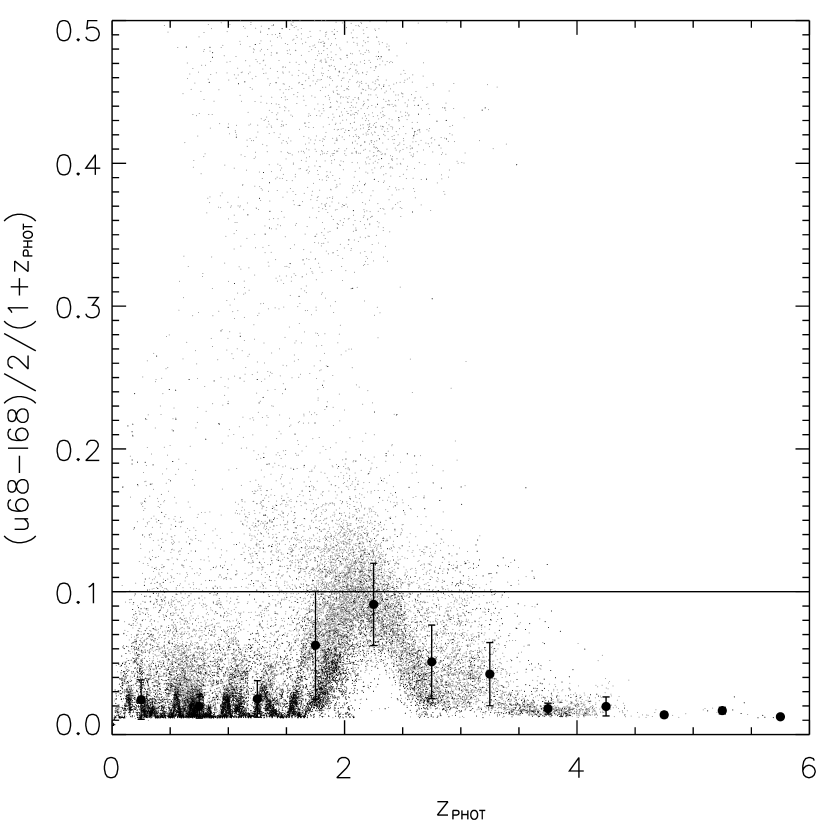
Figure 4.— Illustration of the $z_{\rm phot}$ uncertainties for the combined $z_{\rm phot}$ sample. The $x$-axis shows the best-fitting $z_{\rm phot}$ while the $y$-axis shows $\Delta z_{68}$, the half-width of $z_{\rm phot}$ distribution at the 68% confidence level normalized by $1+z_{\rm phot}$. The horizontal lines correspond to the adopted 10% accuracy per ($1+z_{\rm phot}$) used to exclude less accurate $z_{\rm phot}$ estimates. Black points denote sources in the 5BK3$\sigma$ catalog.

Another illustration of the accuracy of the $z_{\rm phot}$’s is shown in Figure 4, where half of the upper 68% minus the lower 68% confidence ranges in redshift is shown versus photo-$z$. We refer to this as $\Delta z_{68}$$\equiv\frac{\left(z_{+68}-z_{-68}\right)/2}{1+z_{\rm phot}}$, and use it to indicate $z_{\rm phot}$ accuracy. The median and standard deviation of $\Delta z_{68}$ are reported in Table 3 and are shown in Figure 4. As expected, $z\approx 1.8$–2.8 suffers from larger $z_{\rm phot}$ errors due to the absence of a Lyman or Balmer break within the CCD filters, lower sensitivity in the NIR, and in most cases, non-detection in the rest-UV wave bands.

Table 3Summary of Photometric Redshift Uncertainties

	5BK3$\sigma$			5B5$\sigma$
$z$	$N$	Median $\pm$ $\sigma$		$N$	Median $\pm$ $\sigma$
0.0–0.5	3213	0.020$\pm$0.008		6763	0.024$\pm$0.014
0.5–1.0	7029	0.019$\pm$0.009		16172	0.020$\pm$0.008
1.0–1.5	4508	0.019$\pm$0.006		10205	0.025$\pm$0.013
1.5–2.0	4242	0.033$\pm$0.016		12827	0.062$\pm$0.038
2.0–2.5	1673	0.073$\pm$0.029		9257	0.091$\pm$0.029
2.5–3.0	1253	0.044$\pm$0.023		5313	0.050$\pm$0.025
3.0–3.5	522	0.050$\pm$0.032		2388	0.041$\pm$0.021
3.5–4.0	353	0.019$\pm$0.005		1333	0.018$\pm$0.004
4.0–4.5	45	0.020$\pm$0.005		374	0.019$\pm$0.006
4.5–5.0	2	0.017$\pm$0.006		30	0.014$\pm$0.002

Note. — Reported are the median values and standard deviations of the 68% $z_{\rm phot}$ uncertainty: $\Delta z_{68}\equiv(z_{+68}-z_{-68})/2/(1+z_{\rm phot})$.

We did a test excluding $K$-band measurements (our deepest NIR data) for a set of 24,000 $K$-band galaxies detected at $3\sigma$ in at least five bands. We find that the $z_{\rm phot}$ errors increased by 20% (mostly at $z>1$), that the number of outliers (see below) doubled, and the greatest ($\Delta z_{\rm phot}\approx 0.4$) systematic offsets occurred at $z_{\rm phot}=1.3$–2.2. However, for the majority ($\approx$75%) of sources, the photo-$z$’s without $K$ are good to within $\Delta z=\pm 0.05$, particularly at $z_{\rm phot}<1.2$. Therefore, we generate two photo-$z$ samples consisting of bright sources with $K$-band data and those that lack it. The first sample requires a minimum of five-band detection at the $3\sigma$ limit (hereafter 5BK3$\sigma$) with one of the bands being $K$. The second sample consists of at least five-band detection (without any $K$ restrictions) at the $5\sigma$ level (hereafter 5B5$\sigma$). Note that only the measurements from broad and intermediate bands (i.e., narrow bands are excluded) are used to construct these photo-$z$ samples. These samples contain 22853 and 64691 galaxies (after stellar removal). Combining the non-stellar 5B5$\sigma$ and 5BK3$\sigma$ samples yield 65117 galaxies. Since 15-band detection is not available for all sources (e.g., some are undetected in the NUV), we summarize the mixture of detections that we have across 15 bands in Figure 5. Detections in at least 10 wave bands represent 99% of 5BK$3\sigma$ sample and 88.7% of 5B5$\sigma$ sample.

Figure 5.— Summary of the number of band detections for sources in the 5BK3$\sigma$ (left) and 5B5$\sigma$ (right) samples. Optical and NIR bands are included for a total of 15 bands. We have detections in at least 10 wave bands for 99% of 5BK$3\sigma$ sample and 88.7% of 5B5$\sigma$ sample.

We exclude photo-$z$ measurements that are unreliable at the 10% level based on $\Delta z_{68}$. This leaves us with a total sample of 53217 galaxies. Among this accurate photo-$z$ sample, 21768 galaxies are detected at $K$ above 3$\sigma$ while the rest were not. The $z_{\rm phot}$ distribution for both catalogs is illustrated in Figure 6 where 27574 sources are identified to be at $z_{\rm phot}=1$–3 while 21564 are located below $z=1$ and 4079 are above $z=3$. The spike in the distribution at $z_{\rm phot}\sim 1.8$ is an artifact of poorer sensitivity between 1 $\mu$m and 2 $\mu$m that would capture the Balmer/4000 Å break, and is less significant since the photo-$z$ accuracy is lower (see Figure 4). This feature does not effect census results, since the spike is not located near either edge of the redshift window.

Figure 6.— $z_{\rm phot}$ distribution for the combination (solid line) of the 5BK3$\sigma$ and 5B5$\sigma$ samples and only the 5BK3$\sigma$ sample (shaded region). Sources classified as stars were removed and objects with $\Delta z_{68}$$>$ 0.1 were excluded.

Because of the complicated selection for the photo-$z$ samples, one concern is whether derived photo-$z$’s represent the entire population of galaxies. The photo-$z$ samples span the full range of galaxy colors observed in the SDF. Of course, galaxies of lower mass and luminosity are systematically missed at higher redshifts, due to our flux sensitivity limits.

4.2. SED Modeling

To determine physical properties of our galaxies, the Fitting and Assessment of Synthetic Templates (FAST; Kriek et al., 2009) code is used to model the SED. The spectral synthesis models are generated from the Bruzual & Charlot (2003) code, and consist of a star formation history that follows an exponential decay (i.e., a $\tau$ model). For simplicity, we choose $\log{(\tau/{\rm yr})}=$ 8.0, 9.0, and 10.0. These $\tau$ values were selected to include a bursty, intermediate, and roughly constant star formation history. In addition to the star formation history, the grid of models spans a range of $\log{({\rm age/yr})}$, between 7.0 and up to the age of the universe at a given redshift (in increments of 0.1 dex), and dust extinction with $A_{V}=0.0$–3.0 mag with 0.1 mag increments. FAST adopts the Calzetti et al. (2000) dust extinction law, and we only use the solar metallicity models and assume a Salpeter (1955) initial mass function (IMF).

The inputs to the SED fitting are the $z_{\rm phot}$ from EAZY, the photometric measurements, and the total system throughput for each filter (the same as those used in EAZY). The outputs determined from $\chi^{2}$ minimization are the stellar masses, stellar ages, dust reddening ($A_{V}$), star formation rates (SFRs), and $\tau$ values. Narrow-band filter measurements were excluded in the SED modeling (thus up to 17 bands), since FAST has yet to include emission lines.

In the process of modeling the SEDs, we found a problem with the inclusion of IRAC data for 20% of our galaxies. First, the UV extinction-corrected SFRs agree well with those derived from SED modeling with 15 bands (excluding IRAC bands). However, when the IRAC bands were included, the same comparison of SFRs yielded a factor of two higher SFRs from SED modeling. We have not fully understood the cause(s) of this problem, so results using information from the SED modeling are determined with 15 bands instead of 17 bands.

5. Photometric Techniques to Identify $z=1$–3 Galaxies

The following two-color methods are used to select galaxies in the redshift desert: BX, BM, BzK (star-forming and passive), and LBG. The sizes of these galaxy population samples are given in Table 4. Since the $J$-band data are shallower than the $K$, the SDF DRG sample alone is $\sim$200 in size, so we do not include this in the census. We refer readers to Lane et al. (2007, hereafter L07) where a 0.5 deg² NIR survey was conducted and a large sample of bright ($K\lesssim 21$ AB) DRGs was obtained and compared against other NIR-selected galaxies.

Table 4Summary of Photometric Selection Samples

Method	Section	$N$	$N_{z_{\rm phot}}$	$\bar{z}_{\rm phot}$	$z_{\rm phot}$$<1.0$	$z_{\rm phot}$$<0.5$
BX $R_{\rm C}\leq 25.5$	5.1	5585	5070	2.263$\pm$0.39	1282 (25.3%)	1235 (24.4%)
BX $R_{\rm C}\leq 26.0$	5.1	8004	6887	2.240$\pm$0.40	1395 (20.3%)	1326 (19.3%)
BM $R_{\rm C}\leq 25.5$	5.1	6408	6097	1.631$\pm$0.33	943 (15.5%)	778 (12.8%)
BM $R_{\rm C}\leq 26.0$	5.1	8584	7771	1.640$\pm$0.35	1112 (14.3%)	862 (11.1%)
sBzK	5.2	8715	7866	1.939$\pm$0.56	431 ( 5.5%)	179 ( 2.3%)
pBzK	5.2	214	208	1.663$\pm$0.51	1 ( 0.5%)	0 ( 0.0%)
$z\sim 3$ LBG $R_{\rm C}\leq 25.5$	5.3.1	2375	2060	2.913$\pm$0.49	307 (14.9%)	277 (13.4%)
$z\sim 3$ LBG $R_{\rm C}\leq 26.0$	5.3.1	3823	3265	2.862$\pm$0.46	348 (10.7%)	310 ( 9.5%)
$z\sim 2$ LBG $V\leq 25.4$	5.3.2	7878	7663	1.816$\pm$0.47	619 ( 8.1%)	238 ( 3.1%)
$z\sim 2$ LBG $V\leq 26.0$	5.3.2	9745	9397	1.823$\pm$0.45	690 ( 7.3%)	259 ( 2.8%)
$z\sim 1$ LBG	5.3.3	1042	1039	0.834$\pm$0.15	…	…
Total (Shallow)	…	32217	30003	…	3583	2707
Unique (Shallow)	…	20687	18830	…	4120	2481
Total (Faint)	…	40127	36433	…	3977	2936
Unique (Faint)	…	26411	23279	…	4482	2688

5.1. BX/BM Selection

Steidel et al. (2004, hereafter S04) defined BX and BM galaxies by two polygons in the $U_{n}-G$/$G-\mathcal{R}$ color space. For BX, it is $G-\mathcal{R}\geq-0.2$, $U_{n}-G\geq G-\mathcal{R}+0.2$, $G-\mathcal{R}\leq 0.2(U_{n}-G)+0.4$, and $U_{n}-G\leq G-\mathcal{R}+1.0$. The BM selection consists of $G-\mathcal{R}\geq-0.2$, $U_{n}-G\geq G-\mathcal{R}-0.1$, $G-\mathcal{R}\leq 0.2(U_{n}-G)+0.4$, and $U_{n}-G\leq G-\mathcal{R}+0.2$. However, the $U_{n}G\mathcal{R}$ system differs from existing filters of similar wavelengths for the SDF, so a transformation is necessary between $UBVR_{\rm C}i$′ and $U_{n}G\mathcal{R}$. The transformation is derived by using Bruzual & Charlot (2003) spectral synthesis models of star-forming galaxies. Mock galaxies are produced from a grid of synthetic spectra between $z=0.85$ and $z=3.8$ and reddened with the Calzetti et al. (2000) law with $E(B-V)=0.0$–0.4. We also include neutral hydrogen intergalactic medium (IGM) absorption following Madau (1995). Then magnitudes in the $U_{n}$, $G$, $\mathcal{R}$, $U$, $B$, $V$, $R_{\rm C}$, and $i$′ filters are determined for these 540 mock galaxies. Among the artificial galaxies that meet the original BX or BM selection, least-squares fitting is used to represent the $G$ band ($\mathcal{R}$ band) with a combination of $B$ and $V$ ($R_{\rm C}$ and $i$′) such that $U_{n}-G=U-BV$ and $G-\mathcal{R}=BV-R_{\rm C}i\arcmin$, where

$$BV = -2.5\log{\left[\frac{x_{1}f_{B}+(1-x_{1})f_{V}}{3630~{}\mu{\rm Jy}}\right]},\textrm{~{}and}$$ (2)

$$R_{\rm C}i\arcmin = -2.5\log{\left[\frac{x_{2}f_{R}+(1-x_{2})f_{i\arcmin}}{3630~{}\mu\textrm{Jy}}\right]}.$$ (3)

Here, $f_{X}$ is the flux density per unit frequency (erg s^-1 cm^-2 Hz^-1) in band “X.” An illustration of this technique is shown in Figure 7 for BX galaxies.

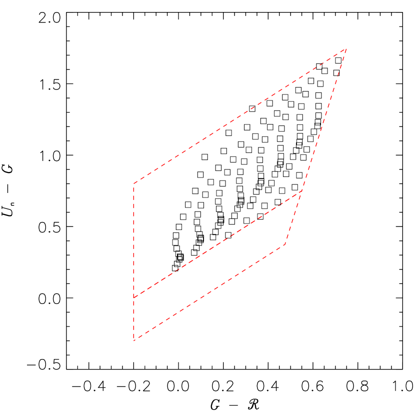
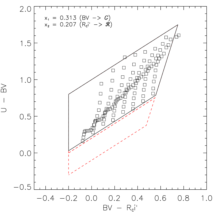
Figure 7.— BX transformation for $U_{n}G\mathcal{R}$ to $UBVR_{\rm C}i\arcmin$. (Left) The originally defined selection of BX galaxies in the $U_{n}G\mathcal{R}$ space. (Right) The $U-BV$ and $BV-R_{\rm C}i\arcmin$ colors for these BX galaxies, as determined by Equations (2) and (3) with $x_{1}=0.314$ and $x_{2}=0.207$. The solid black lines refer to the final BX selection (see Equations (4)–(7)) while the red dashed lines illustrate the S04 selection. These plots indicate a proper transformation has been made to select all BX galaxies. These transformation is further discussed in Section 5.1. (A color version of this figure is available in the online journal.)

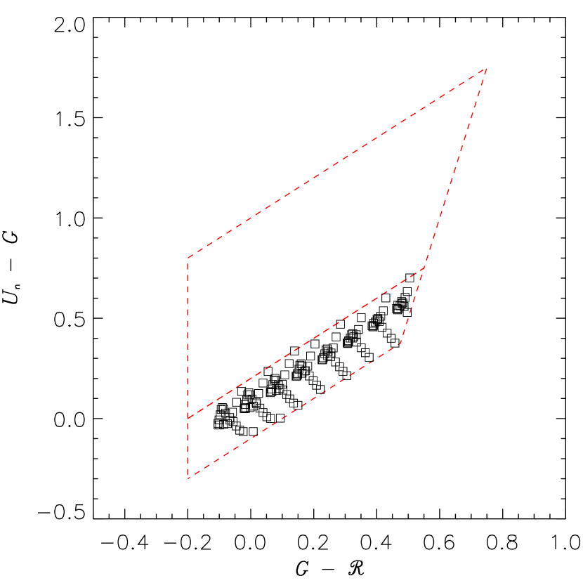
Figure 8.— Similar to Figure 7, but illustrated here for BM galaxies. These plots indicate a reasonable transformation for BM galaxies when using the BX transformation except for $z\sim 1$ BM galaxies. We adopt a different selection for BM galaxies, as shown by the solid black lines (see Equations (8)–(12)) compared to the S04 selection illustrated by the red dashed lines. Further discussion of the transformation is available in Section 5.1. (A color version of this figure is available in the online journal.)

While different values of $x_{1}$ and $x_{2}$ can be adopted for the BX ($x_{1}=0.314$ and $x_{2}=0.207$) and BM ($x_{1}=0.491$ and $x_{2}=0.790$) selections, the net result is that some BX galaxies would also meet the BM selection and vice versa. However, the BX and BM galaxies occupy distinct regions in the default $U_{n}G\mathcal{R}$ plane, so only one transformation set can be used to identify the two galaxy populations simultaneously. As a compromise, we decided to adopt the BX $x_{1}$–$x_{2}$ transformation, since it occupies the region between the BM and $U$-dropout techniques. With this approach, the BX selection parallelogram remains roughly the same, while the BM and $U$-dropout selection regions are modified. The only modification that we make to the BX selection is to move the lower bound up by 0.03 mag in $U-BV$:

$$BV-R_{\rm C}i\arcmin \geq -0.2,$$ (4)

$$U-BV \geq BV-R_{\rm C}i\arcmin+0.23,$$ (5)

$$BV-R_{\rm C}i\arcmin \leq 0.2(U-BV)+0.4,\textrm{\, and}$$ (6)

$$U-BV \leq BV-R_{\rm C}i\arcmin+1.0.$$ (7)

It should be noted that the BM transformation did change significantly when adopting the BX photometry transformation (see Figure 8). It now spans a wider range in $BV-R_{\rm C}i\arcmin$ color, so more $z<1$ sources could potentially contaminate our BM sample at the cost of identifying $z>1$ BM galaxies. As a compromise, we choose not to extend the selection region to encompass the lowest-redshift BM galaxies, in order to exclude some low-$z$ interlopers. This may sound alarming, but it is expected, since the original BM selection spanned a small range of $G-R$ color for a given $U_{n}-G$ color. Thus scatter from photometric uncertainties causes missed faint $z>1$ galaxies and the inadvertent inclusion of low-$z$ interlopers. The final selection that we use for BM galaxies is

$$BV-R_{\rm C}i\arcmin \geq -0.2,$$ (8)

$$U-BV \geq -0.1,$$ (9)

$$BV-R_{\rm C}i\arcmin \leq 0.382(U-BV)+0.853,$$ (10)

$$BV-R_{\rm C}i\arcmin \leq 0.70(U-BV)+0.280,\textrm{\, and}$$ (11)

$$U-BV \geq BV-R_{\rm C}i\arcmin+0.23.$$ (12)

Figure 9.— $U-BV$ and $BV-R_{\rm C}i\arcmin$ colors to select BX and BM galaxies. Triangle points are sources that are undetected in $U$ at $1\sigma$. Black lines indicate the selection boxes for BX (top) and BM (bottom). Selection is performed for $R_{\rm C}\leq 25.5$ mag.

The $U-BV$ and $BV-R_{\rm C}i\arcmin$ colors for SDF galaxies are shown in Figure 9 for the selection of BX and BM galaxies. Following Steidel et al. (2003), we defined a non-detection in the $U$ band when its flux falls below the 1$\sigma$ limit.

In total, 6280 BX (5585 after stellar removal) and 6776 BM (6408 after stellar removal) galaxies are identified with $R_{\rm C}\leq 25.5$. In Section 6.2, we also discuss the BX and BM samples with $R_{\rm C}\leq 26.0$, which consist of 8699 BX (8004 after stellar removal) and 8952 BM galaxies (8584 after stellar removal). In Figure 10, the photometric redshift distributions of the BX and BM samples are illustrated. Also overlaid are the spectroscopic redshift distributions from S04 and Reddy et al. (2008), which demonstrates the accuracy of EAZY at $z\sim 2$ and shows that the filter transformations did indeed approximate the original BX and BM definitions. Further evidence that the transformation was done correctly is the surface density of BXs, which is shown in Figure 11. It is compared with measurements reported by Reddy et al. (2008) and shows good agreement over a range of $\sim$3 mag.

Although not illustrated in Figure 10, a subset of the BX and BM samples have $z_{\rm phot}=0.1$–0.5. The BX (BM) $R_{\rm C}\leq 25.5$ sample has 1235 (778) with $z_{\rm phot}\leq 0.5$ corresponding to 24.4% (12.8%). These numbers decrease to 19.3% (11.1%) when considering the sample with $R_{\rm C}\leq 26.0$. These galaxies have accurate $z_{\rm phot}$’s ($\Delta z_{68}$ $<$ 4%), so it cannot be argued that these galaxies are at $z>1$. Furthermore, we inspected the $B-z\arcmin$ and $z\arcmin-K$ colors and find that these objects occupy a region below the star-forming BzK selection (see Section 5.2), which provides further evidence that they are at $z\lesssim 1.3$ (i.e., the Balmer/4000 Å break is observed in the optical). The full $z_{\rm spec}$ distributions for BX and BM galaxies were not provided in S04, but the $z_{\rm spec}<1.0$ interloper statistics were stated to be 17.1% and 5.8% for BX and BM ($\mathcal{R}\leq 25.5$) galaxies, respectively. G07 found similar results to ours for their BX sample.

Figure 10.— Distribution of $z_{\rm phot}$’s for the UV-selected BX, BM, and $U$-dropout (solid lines) compared to the spectroscopic samples of S04 or Reddy et al. (2008). Galaxies were selected down to $R_{\rm C}=25.5$ mag.

Figure 11.— Observed surface density of BX galaxies (left) and $U$-dropouts (right) shown as filled (exclude stars) and open (include stars) squares. There is good agreement with the filled circles from Reddy et al. (2008).

5.2. BzK Selection

Figure 12.— $B-z\arcmin$ and $z\arcmin-K$ colors for $\sim$25,000 sources detected in the $K$ band above $3\sigma$. Star-forming BzKs are identified as those above the slanted line (BzK = $-0.2$) while the selection of passive BzKs is through a combination of the horizontal and the slanted lines. Triangle points indicate $K$-band sources that are undetected in the $B$ band at $3\sigma$ (lower limit on the $B-z\arcmin$ color).

Daddi et al. (2004) defined star-forming BzK (sBzK) galaxies as those with $BzK\equiv(z-K)-(B-z)\geq-0.2$ with detection required in $B$ and $K$. This corresponds to the solid line in Figure 12, which has 8715 star-forming BzK (hereafter sBzK) galaxies falling above it. In addition, the passive BzK (pBzK) selection, which requires $BzK<-0.2$ and $z-K\geq 2.5$, yields 228 galaxies (214 after stellar removal) with $z=1$–1.5. The photo-$z$’s of the pBzK and sBzK populations are shown in Figure 13. They show good agreement with photo-$z$’s derived for BzK galaxies in the COSMOS field (McCracken et al., 2010). The COSMOS BzK sample probed $K<23.0$ while our sample reaches $K\sim 24.0$. We find better agreement with COSMOS at the $z_{\rm phot}=1.7$–3.0 range when limiting our sample to $K<23.0$. The COSMOS and SDF samples of BzK galaxies independently confirm that sBzK galaxies are at $z\approx 1.5$–2.5 and pBzK galaxies are at $z\approx 1.0$–1.5.

Figure 13.— $z_{\rm phot}$ distribution for 7866 of 8715 sBzK galaxies (left) and 208 of 228 pBzK galaxies (right) indicated by the solid lines. The dotted line represents sBzK galaxies with $K<23$ mag to compare with the photo-$z$ distribution of sBzK galaxies from the COSMOS survey (McCracken et al., 2010), which are overlaid as dashed lines. The COSMOS distributions have been normalized to the peak in the SDF $K<23$ mag $z_{\rm phot}$ distributions.

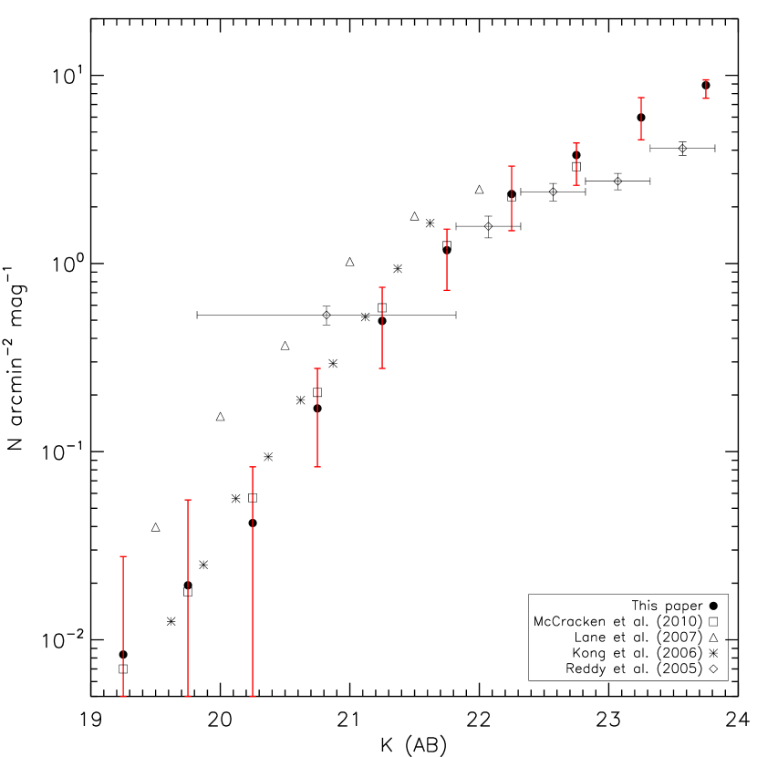
Figure 14.— Surface density of sBzK galaxies in the SDF (filled circles) compared to other surveys: McCracken et al. (2010, squares), L07 (triangles), Kong et al. (2006, asterisks), and R05 (diamonds). Red error bars illustrate the minimum and maximum surface density for eight independent 8$\farcm$5$\times$8$\farcm$5 fields in the SDF. (A color version of this figure is available in the online journal.)

In Figure 14, we plot the surface density of the SDF sBzK galaxies and previous sBzK surveys (Reddy et al., 2005; Kong et al., 2006; Lane et al., 2007; McCracken et al., 2010). We find that our measured surface density for sBzK is consistent with those reported in McCracken et al. (2010) down to their $K$-band depth of $\sim$23.0 AB. Kong et al. (2006) show a higher surface density but is consistent with the photometric scatter. L07 also find a higher surface density, although McCracken et al. (2010) pointed out that this is likely due to a photometric calibration issue. Finally, the surface density of R05’s sBzKs is consistent with ours for $K<23$ AB, and then is lower than ours by a factor of at most two. We will discuss this discrepancy at faint $K$ in Section 6.3.

5.3. LBG Selection

The above techniques were designed to select $z=1$–3 galaxies when the Lyman break technique is not detectable with optical photometry. This has now changed since L09 used ultraviolet imaging for the first survey of $z\sim 2$ LBGs in the SDF. To fully span the $z=1$–3 era with the Lyman break technique, we select $U$-, NUV-, and FUV-dropouts. We will interchangeably use $U$/NUV/FUV-dropouts and $z\sim 3$/2/1 LBGs to refer to the Lyman-limit break selected sources.

5.3.1 $U$-dropouts

Using the $UBVR_{\rm C}i\arcmin$ to $U_{n}G\mathcal{R}$ transformation described in Section 5.1, we identify $U$-dropouts in a similar manner as Steidel et al. (2003): $U-BV\geq-0.1$, $BV-R_{\rm C}i\arcmin\leq 0.95$, and $U-BV\geq BV-R_{\rm C}i\arcmin+1.0$. A modification is made to the right edge by shifting it 0.15 mag bluer in $BV-R_{\rm C}i\arcmin$. This selection spans the region above the BX selection window, as illustrated in Figure 15. We find 2578 $U$-dropouts with $R_{\rm C}\leq 25.5$ (2375 after stellar removal). The surface density for our $U$-dropouts (see Figure 11) is similar to those reported by Reddy et al. (2008). Finally, we compare the $z_{\rm phot}$ for $U$-dropouts against the Reddy et al. (2008) sample in Figure 10 and find good agreement, which further supports the idea that our selection is probing the same galaxies identified by Steidel et al.

Figure 15.— $U-BV$ and $BV-R_{\rm C}i\arcmin$ colors to select $U$-dropout galaxies. Triangle points are sources that are undetected in $U$ at $1\sigma$. The selection boxes for BXs, BMs, and $U$-dropouts are shown.

5.3.2 NUV-dropouts

The selection of NUV-dropouts is discussed in L09. The definition is: $NUV-B\geq 1.75$, $B-V\leq 0.50$, and $NUV-B\geq 2.4(B-V)+1.15$. In defining the selection criteria, we used a spectral synthesis model that is similar to that used for selecting $U$-dropouts. The range of dust reddening probed by the above color criteria, $E(B-V)=0.0$–0.4, is fairly similar to those selected by Steidel et al. should galaxies that span this full range exists. Thus, the main difference between the two populations of LBGs is the redshift sensitivity. This statement, of course, assumes that there is no evolution in the properties (e.g., dust) of LBGs between $z\sim 3$ and $z\sim 2$.

There are two corrections that we make to the previous selection. First, a source is considered undetected in the NUV when it is below the 1$\sigma$ threshold. Previously, we adopted $3\sigma$ to be conservative; however, we decided to be consistent with Steidel et al. (2003) for the final selection of all Lyman-limit galaxies. This will shift points in Figure 9 of L09 by 1.2 mag redder in $NUV-B$. Second, we failed to apply an aperture correction for undetected sources in L09. The aperture correction that we adopted previously was 1.81, and our latest calculation, which we now use, indicates 1.85, which leaves a 0.6 mag offset in the $NUV-B$ colors for faint galaxies.

By adopting a $1\sigma$ threshold in the NUV, the $z\sim 2$ UV luminosity function discussed in L09 changes. To first order, the completeness corrections were underestimated at $z=2$–2.5, since some of the simulated galaxies that fell below our $NUV-B=1.75$ mag will now enter the $z\sim 2$ LBG selection region. However, by adopting a lower threshold, more sources will also enter our selection region that were bluer than $NUV-B=1.75$ mag. We note that the comparison between BX/BM and $z\sim 2$ LBG is more robust in this paper than in L09 since a direct comparison is made using the same data.

The $NUV-B$ and $B-V$ colors for $V<25.4$ sources are shown in Figure 16, and 8574 NUV-dropouts (7878 after stellar removal) are identified. Recall that the NUV fluxes were obtained by PSF-fitting bright sources in order to obtain reliable fluxes for faint, confused sources. If this step was not performed, the NUV-dropout sample would be $\approx$30% smaller. This is similar to the fraction of missed mock LBG galaxies in the Monte Carlo simulation of L09. In Section 6.2, we also discuss the NUV-dropout sample with $V\leq 26.0$, which consists of 10441 sources (9745 after stellar removal). The $z_{\rm phot}$ distribution is shown in Figure 16, and indicates that the selection mostly identifies galaxies at $z=1.5$–2.5, with 25.4% contamination from $z<1.5$ interlopers.

Figure 16.— (Left) The selection of NUV-dropouts with $NUV-B$ and $B-V$ colors with $V\leq 25.4$. Triangle points indicate sources with $1\sigma$ limits in the NUV band. (Right) The $z_{\rm phot}$ distribution for most NUV-dropouts.

5.3.3 FUV-dropouts

Studies (e.g., Burgarella et al., 2007) have used GALEX FUV imaging to select $z\sim 1$ LBGs. The selection of FUV-dropouts is currently best described in conference proceedings. The selection which has been adopted is $FUV-NUV\geq 2.0$, $NUV-U\leq 1.4$, and $FUV-NUV\geq 1.05(NUV-U)+2.52$. The $FUV-NUV$ and $NUV-U$ colors are shown in Figure 17. We identified 1067 FUV-dropouts (1042 after stellar removal) with $U<25.0$ mag. We find that the $z_{\rm phot}$ distribution is skewed towards $z\sim 0.7$–0.8 (see Figure 17). While FUV-dropouts have been claimed to be at $z\sim 1$, the Lyman continuum breaks occurs at the FUV filter center at $z=0.68$, reducing the flux by half. This peak is not surprising given (1) the current UV sensitivity and (2) the majority of $z\sim 1$ galaxies have $U>25$ mag.

Figure 17.— (Left) The selection of FUV-dropouts with $FUV-NUV$ and $NUV-U$ colors. Triangle points indicate sources with $1\sigma$ limits in the FUV band. (Right) The $z_{\rm phot}$ distribution for almost all FUV-dropouts.

5.4. Summary

We used color selection to identify 5585 BXs (8004 $R_{\rm C}\leq 26.0$), 6408 BMs (8584 $R_{\rm C}\leq 26.0$), 8715 sBzKs, 214 pBzKs, 2375 $U$-dropouts (3823 $R_{\rm C}\leq 26.0$), 7878 NUV-dropouts (9745 $V\leq 26.0$), and 1042 FUV-dropouts for a total of 32217 (adopting a shallower limit on $R_{\rm C}$ or $V$) or 40127 (adopting a fainter limit on $R_{\rm C}$ or $V$) galaxies potentially at $z\approx 1$–3. However, since there is overlap between the different color-selected samples, the non-redundant sample contains 20687 (18830 with $z_{\rm phot}$) and 26411 (23279 with $z_{\rm phot}$) galaxies in the Shallow and Faint samples, respectively.

6. Results

In this section we begin by discussing the properties of galaxies selected using a given photometric technique. Then we compare the different color selections to discuss sample overlap and the selection bias associated with each technique. We then compare the color-selected samples against photo-$z$’s to estimate the completeness of using these techniques in acquiring a census of star-forming galaxies at $z=1$–3.

6.1. The Physical Properties of $z=1$–3 Galaxies

Using the color selection samples with $z_{\rm phot}$ and information from SED modeling, we illustrate in Figure 18 the efficiency of these photometric techniques in terms of the relative fraction of the total number. We find that the BX and BM methods identify 60%–80% of galaxies at the peak of their $z_{\rm phot}$ distributions (i.e., where they are most sensitive). The $U$-dropout technique identifies 80% of galaxies at $z\sim 3$. However, this is optimistic since our “Total” sample is missing low-mass $z\sim 3$ red/dusty galaxies should they exist. Likewise, it appears that the NUV-dropout technique has similar efficiency as the BX/BM method with a redshift coverage that spans the redshift of BX and BM galaxies. LBGs at $z\sim 1$ would require UV imaging at $\approx$1800 Å (between the FUV and NUV band). Finally, the star-forming BzK selection probes a wider range in redshift: capturing at least 40% of galaxies at $z>3$ and as much as $\sim$70% at $z\sim 1.5$.

Figure 18 also illustrates that the very different methods to identify galaxies at this epoch are complementary, and that no single method identifies all galaxies. The union of the different color selection techniques does yield a comprehensive galaxy census of $z=1$–3.

Figure 18.— Fraction of the Shallow sample versus redshift for the different color selection techniques: NUV-dropout (solid; black), sBzK (dashed; red), pBzK (dotted; orange), BX (dot-dashed; green), BM (dot-dot-dashed; blue), and $U$-dropout (long-dashed; purple). We illustrate (in a given redshift bin) the fraction in terms of the total number of galaxies. (A color version of this figure is available in the online journal.)

To further understand the selection bias of these techniques, we illustrate in Figure 19 the distribution of dust reddening, stellar mass, SFR, and stellar ages for the BX, BM, sBzK, pBzK, and NUV-dropout samples. These distributions are normalized to the census of these techniques. The majority of galaxies with stellar masses above $6\times 10^{9}$ $M_{\sun}$ are acquired with the sBzK technique. UV selection methods are more efficient at selecting lower-mass galaxies. The BzK technique is also able to identify the oldest galaxies and those with high dust extinction. UV techniques find young galaxies with little dust extinction and typical SFRs of 1–10 $M_{\sun}$ yr^-1. The $z\sim 2$ LBG population appears to span a wider range of dust reddening compared to the BX/BM method. We attribute this to the (1) larger range in rest-UV colors ($B-V<0.5$ mag spans a wider $G-\mathcal{R}$ color compared to the $G-\mathcal{R}$ color of BX/BM galaxies) and (2) an ability to select massive galaxies. We discuss this further in Section 6.2.1. Figure 19 also shows that the most actively star-forming galaxies will be identified using either the sBzK or NUV-dropout method. However, 66% of the color-selected $z_{\rm phot}=1$–3 census consists of galaxies with SFRs between a few and 30 $M_{\sun}$ yr^-1, and 70% of this fraction is captured using the BX/BM method with $R_{\rm C}\leq 25.5$ mag.

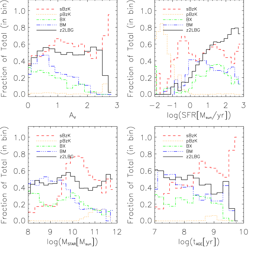
Figure 19.— Physical properties of $z=1$–3 galaxies. The distribution of A_V (top left), $\log({\rm SFR}[M_{\sun}~{}{\rm yr}^{-1}])$ (top right), $\log(M_{\rm star}[M_{\sun}])$ (bottom left), and $\log({\rm age[yr]})$ (bottom right) for the different population. Color and line-style conventions follow those in Figure 18. The $U$-dropouts are not shown since most of them are at $z_{\rm phot}\gtrsim 3.0$. (A color version of this figure is available in the online journal.)

6.2. A Direct Comparison of Color Selection Techniques

Table 5Summary of Photometric Selection Census Surveys

Properties	Field
	GOODS	MUSYC	CDF-S	UDS	SDF
Refer.	R05	Q07	G07	L07	L11
Area	72.3	413	90.2	2013	720
$N_{\rm total}$	931	2959	2630	12503	20687
$R$ depth	25.5	25.5	25.5	…	25.5
$K$ depth	23.0	$\approx$23.45	23.5	22.5	24.2
$z_{\rm phot}$	No	9-band	13-band	No	20-band
$z_{\rm spec}$	Yes	No	$\sim$1000	No	…
BX	620	532	1345	No	5585
BM	…	741	…	No	6408
$z3$LBG	No	401	…	No	2375
sBzK	221	2213	747	6736	8715
pBzK	17	326	89	816	214
DRG	73	480	179	330	No
ERO	No	No	No	4621	No
$z2$LBG	No	No	No	No	7878

Note. — “L11” refers to this paper. Areas are in arcmin².

Previous studies (; ; ; ) have also investigated the completeness of photometric selection and the selection bias in the GOODS-N, GOODS-S/CDF-S, MUSYC, and UKIRT fields. However, as illustrated in Table 5, each study has its own advantages and disadvantages in terms of area coverage, color selection used, and redshift accuracy. Since these surveys could not identify $z\sim 2$ LBGs, comparisons were made between the BX/BM/$U$-dropout methods and the BzK/DRG methods given, and it was assumed that BX/BM’s are lower-redshift analogs of $z\sim 3$ LBGs. We discuss the overlap between BX/BM and $z\sim 2$ LBGs in Section 6.2.1. In previous studies, the term “LBG” is used to refer to the selection of $U$-dropouts. We make a clear distinction between the two.

A summary of the color selection sample overlap is provided in Table 6, along with the average $z_{\rm phot}$, $E(B-V)$, stellar age, stellar mass, and SFR. We have created a 6-digit binary index to refer to the sample overlap. Each digit refers to a specific galaxy population in the following order: pBzK, sBzK, BM, BX, $U$-dropout, and NUV-dropout. So for example, galaxies that simultaneously satisfy the color criteria of sBzK, BX, and NUV-dropout are denoted as “010101”. The diagram in Figure 20 illustrates the sample overlap. The BX, BM, and $U$-dropouts do not overlap, given the mutually exclusive color selection. This is also the case for the passive and star-forming BzK-selected galaxies. Note that we have not placed any restrictions on the optical ($K$-band) magnitudes for NIR-selected (UV-selected) galaxies for this table and this overlap diagram. We discuss the overlap with such restrictions in Section 6.2.1, to compare with previous estimates.

Table 6Summary of Photometric Technique Overlap

Type	$N$	$z$	$E(B-V)$	$\log{(\rm{M})}$	$\log{({\rm SFR})}$	$\log{(t_{\rm age})}$
			(mag)	($M_{\sun}$)	($M_{\sun}$ yr-1)	(yr)
100000	207	1.66$\pm$0.51	0.18$\pm$0.14	10.93$\pm$0.39	–1.66$\pm$1.86	9.00$\pm$0.23
010000	2525	1.85$\pm$0.66	0.23$\pm$0.17	10.14$\pm$0.70	0.78$\pm$0.69	8.78$\pm$0.56
011000	609	1.57$\pm$0.36	0.15$\pm$0.09	9.69$\pm$0.50	0.87$\pm$0.42	8.56$\pm$0.50
010100	559	2.29$\pm$0.46	0.16$\pm$0.12	10.15$\pm$0.43	1.13$\pm$0.52	8.61$\pm$0.44
010010	444	2.84$\pm$0.41	0.13$\pm$0.11	10.42$\pm$0.34	1.26$\pm$0.44	8.80$\pm$0.40
010001	530	1.57$\pm$0.17	0.21$\pm$0.14	10.42$\pm$0.59	1.20$\pm$0.65	8.54$\pm$0.47
011001	1618	1.73$\pm$0.19	0.15$\pm$0.09	9.89$\pm$0.39	1.13$\pm$0.48	8.41$\pm$0.45
010101	1325	2.21$\pm$0.32	0.14$\pm$0.10	10.07$\pm$0.42	1.33$\pm$0.44	8.53$\pm$0.46
010011	77	2.50$\pm$0.35	0.13$\pm$0.11	10.88$\pm$1.28	1.65$\pm$0.75	8.74$\pm$0.48
000001	1266	1.23$\pm$0.40	0.27$\pm$0.16	9.78$\pm$0.82	1.21$\pm$0.82	8.19$\pm$0.70
001001	1470	1.73$\pm$0.26	0.15$\pm$0.09	9.58$\pm$0.80	1.14$\pm$0.54	8.23$\pm$0.80
000101	1043	2.29$\pm$0.29	0.10$\pm$0.08	9.50$\pm$0.81	1.15$\pm$0.45	8.15$\pm$0.78
000011	95	2.59$\pm$0.25	0.08$\pm$0.11	9.82$\pm$1.46	1.38$\pm$1.12	8.14$\pm$0.63
001000	1622	1.47$\pm$0.40	0.12$\pm$0.09	9.17$\pm$0.62	0.71$\pm$0.48	8.26$\pm$0.66
000100	908	2.30$\pm$0.53	0.10$\pm$0.10	9.43$\pm$0.77	0.86$\pm$0.50	8.22$\pm$0.70
000010	1167	2.99$\pm$0.51	0.07$\pm$0.09	9.75$\pm$0.69	1.05$\pm$0.59	8.33$\pm$0.54

Note. — Average properties are reported. The first column is a 6-digit binary flag with each digit referring to a specific galaxy population in the order of pBzK, sBzK, BM, BX, $U$-dropout, and NUV-dropout. See Section 6.2 for further description. Sources with $z_{\rm phot}<0.5$ are excluded.

Figure 20.— Diagram illustrating photometric galaxy sample overlap for the Shallow sample. Redshift increases to the right. Statistics are provided in each box including the size of a given sample, and the fraction relative to the full and each individual sample. “K flag” refers to sources that fall in lower sensitivity regions, so they cannot be classified in the BzK diagram. We exclude sources with $z_{\rm phot}<0.5$.

6.2.1 Sample Overlap: Color–Color Plots

Table 7Summary of Sample Overlap: NIR Selection

Type	FoV Limited	$K>3\sigma$	Total
BX	3493	2065	1995 (96.6%)
BM	4670	2955	2265 (76.6%)
$z$$\sim$3 LBG	1701	824	559 (67.8%)
$z$$\sim$2 LBG	6249	4784	3602 (75.3%)

Note. — Sources with $z_{\rm phot}$$<0.5$ have already been excluded.

Table 8Summary of Sample Overlap: $U_{n}G\mathcal{R}$ Method

Type	$R<25.5$	BX	BM	$z$$\sim$3 LBG	Total
sBzK	6201	1995	2265	559	4819 (77.7%)
$z$$\sim$2 LBG	7603	2465	3151	180	5796 (76.2%)

Table 9Summary of Sample Overlap: NUV-dropout Method

Type	$z_{\rm phot}\geq 1.5$	$V<25.4$	Total
BX	3697	2934	2337 (79.7%)
BM	3499	2886	2512 (87.0%)
sBzK	6300	4095	3160 (77.2%)

To further understand and illustrate the selection effects of these techniques, we plot where each galaxy population/technique (e.g., BX) falls in the color–color selection of another (e.g., BzK). We first discuss the BzK selection, followed by the $U_{n}G\mathcal{R}$ methods, and finally the selection that we have developed to identify $z\sim 2$ LBGs. Note that the numbers below have excluded interlopers with $z_{\rm phot}<0.5$ (unless otherwise indicated). When computing the overlap fraction and providing the two-color distribution of sources, we place limits on either the $V$, $R_{\rm C}$, or $K$, as we did when we generated the high-$z$ photometric samples.

A detailed summary of the statistics reported in this section is provided in Tables 7–9.
Near-IR selection. The $B-z\arcmin$ and $z\arcmin-K$ colors for BXs, BMs, NUV-dropouts, and $U$-dropouts are shown in Figure 21. When the BX, BM, $U$-dropout, and NUV-dropout samples (1) are restricted to the region of sensitive $K$ photometry, (2) exclude sources with $z_{\rm phot}<0.5$, and (3) only consider sources detected above $3\sigma$ in $K$, we find that 96.6% of BXs, 76.6% of BMs, 67.8% of $U$-dropouts, and 75.3% of NUV-dropouts meet the sBzK selection, which indicates that sBzK method is capable of selecting almost all high-$z$ UV-selected galaxies having $K\lesssim 24$ mag. Table 7 provides more information regarding these statistics. We note that if we did not exclude objects with $z_{\rm phot}<0.5$, the overlap fraction would be 75.9% (BX), 68.5% (BM), 59.6% ($U$-dropout), and 73.5% (NUV-dropout). More than two-thirds of $U$-dropouts with $K$-band detections are also identified as sBzK. The redshift where the Balmer/4000 Å break enters the $K$-band window is $z\approx 4$, so extremely deep $K$-band imaging ($K=25$–26) can yield mass-limited samples of $z\lesssim 4$ galaxies with stellar masses above $\sim 10^{10}$ $M_{\sun}$. These high-$z$ sBzKs were also seen by G07, but in smaller numbers. Unfortunately, they did not report a sBzK–$U$-dropout overlap fraction to compare to ours. G07 did find that $>86\%$ of $z>1.4$ BX/BM galaxies are sBzK galaxies, which is consistent with the above number. Q07 determined that 80% of BX/BM/$U$-dropout galaxies (regardless of $z_{\rm phot}$) are sBzK-selected, which agrees with our number without any $z_{\rm phot}$ constraints. Likewise, similar numbers were reported by R05.

The majority of sources that are missed by the sBzK method are BM and NUV-dropout galaxies. We find that these non-sBzK galaxies have characteristic $z_{\rm phot}\approx 1.9$, $E(B-V)\approx 0.1$, stellar masses of $\sim 10^{10}$ $M_{\sun}$, SFRs of $\sim$10 $M_{\sun}$ yr^-1, and stellar ages of $3\times 10^{8}$ yr. It is not surprising that the BzK technique misses blue galaxies, since it is more sensitive to redder galaxies.

None of the BX, BM, $U$-dropout, and NUV-dropout sources are classified as a passive BzK, indicating that pBzK galaxies represent a completely separate population. This was also seen by Q07. We further discuss this in the Appendix.

The fraction of sBzK galaxies that are BXs, BMs, or $U$-dropouts varies with $K$-band magnitude, with larger overlap at fainter $K$ (see Figure 22). This is to be expected, as the UV selection techniques probe less reddened and young galaxies that are typically of lower masses. Our measurements agree with those of R05 at $K\approx 22$–23 mag and extend toward $K\approx 24$ to show a slightly larger fraction of overlap. However, our sBzK–BX/BM/$U$-dropout overlap fraction is noticeably lower for $K<22.0$ mag. We find that the overlap fraction for a magnitude bin of $20<K<22$ is typically 23% with 1$\sigma$ variation of 10% when dividing our SDF survey into cells of 8$\farcm$5 $\times$ 8$\farcm$5, which are similar to the surveyed area of R05. Thus, the discrepancy could be explained by clustering of such galaxies and their smaller area coverage.

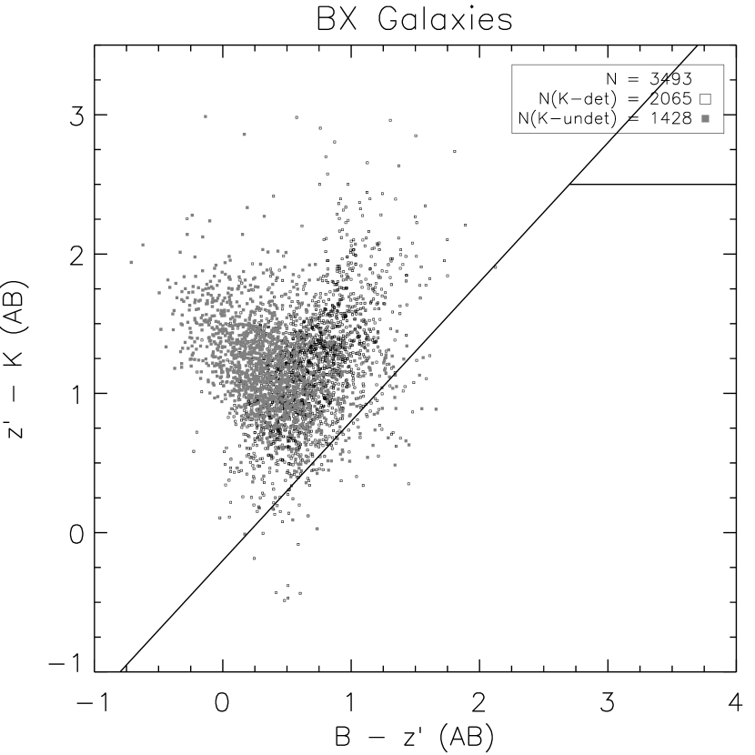
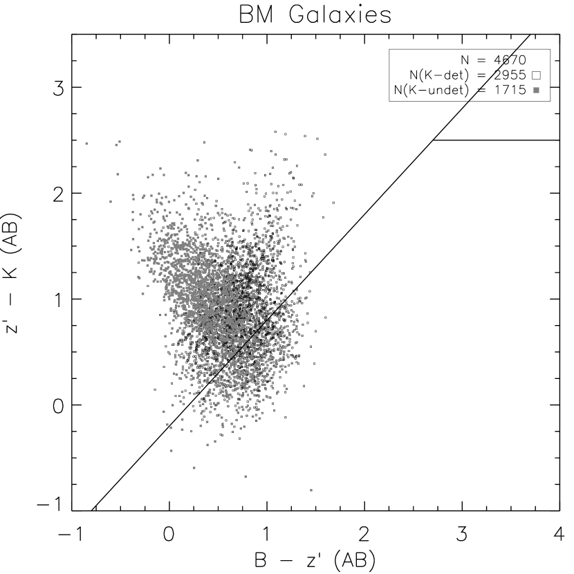
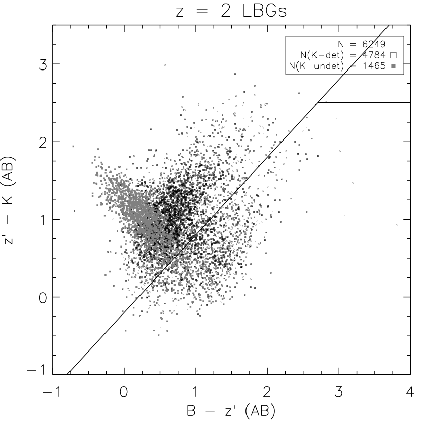
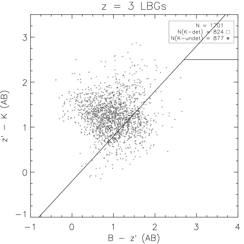
Figure 21.— Sample overlap: $B-z\arcmin$ and $z\arcmin-K$ colors for BX galaxies (upper left), BM galaxies (upper right), NUV-dropouts (lower left), and $U$-dropout galaxies (lower right). Sources shown as black are those with $>3\sigma$ detection in $K$, while those in gray are sources undetected in $K$ (upper limits on their $z\arcmin-K$ color). Note that the axis scales differ from those in Figure 12.

Figure 22.— Fraction of $z_{\rm phot}\geq 1.5$ sBzK galaxies that meets the BX (diamonds), BM (triangles), $U$-dropout (squares) or NUV-dropout (crosses) selection. The combination of the first three UV selection techniques is shown as filled circles. The sample overlap increases towards lower $K$-band luminosities, which is expected given the selection bias that UV techniques target lower mass galaxies. Overlaid in asterisks are estimates from R05. This figure also illustrates that the Lyman break technique is able to identify many massive $z\sim 2$ galaxies, which the BX/BM method misses.

Non-ionizing UV continuum selection: the $U_{n}G\mathcal{R}$ method. For the selection of BX, BM, and $U$-dropout galaxies, the BzK galaxies and $z\sim 2$ LBGs are plotted on the $U-BV$ and $BV-R_{\rm C}i\arcmin$ color space in Figure 23. We find that among the sBzK galaxies with $R_{\rm C}\leq 25.5$ and $z_{\rm phot}>0.5$, 32.2% are BXs, 36.5% are BMs, and 9.0% are $U$-dropouts, for a total overlap of 77.7%. Detailed information of the overlap is provided in Table 8. Q07 determined $\sim$65% for this fraction. To understand this small yet noticeable difference, we point out that our sample probes much fainter $K$ magnitudes than they did, by $\approx$1 mag. Since the majority of BX/BM galaxies have low stellar masses, many of them are faint in $K$. As a result, our survey is more complete in mass, and is weighted more toward the lower luminosity galaxies. We see this from the slightly higher overlap fraction in Figure 22 for $K_{\rm AB}>23.0$ mag. Likewise, among NUV-dropouts with $R_{\rm C}\leq 25.5$ and $z_{\rm phot}>0.5$, 32.4% are BXs, 41.4% are BMs, and 2.4% are $U$-dropouts, for a total overlap of 76.2%. The small overlap between NUV-dropouts and $U$-dropouts is to be expected, since we intended to exclude $z\gtrsim 2.7$ galaxies with the $B-V\leq 0.5$ mag criterion (see L09, ).

Recall that S04 defined the BX/BM selection to identify $z\sim 2$ galaxies that are analogous to $z\sim 3$ LBGs. The presence of this large overlap shows that this statement is mostly true. We find, however, that the LBG selection identifies a significant population of redder and more massive galaxies: at least half of the $K<21.5$ sBzK galaxies are selected using the NUV-dropout method. This was previously illustrated in Figure 21 with the NUV-dropouts spanning redder $B-z\arcmin$ and $z\arcmin-K$ colors compared to the BX galaxies, and again in Figure 22, where the NUV-dropout method identified more $K$ bright galaxies compared to BX/BM. It also explains the cluster of points at $BV-R_{\rm C}i\arcmin=0.5$–1.3 mag, which is also seen for sBzK galaxies.

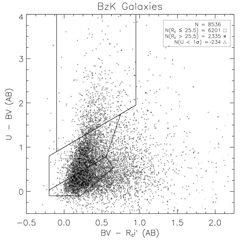
Figure 23.— Sample overlap: $U-BV$ and $BV-R_{\rm C}i\arcmin$ colors for BzK galaxies (left) and $z\sim 2$ LBGs (right). Sources shown as black are those with $R_{\rm C}\leq 25.5$ while those in gray are fainter than $R_{\rm C}=25.5$. Triangle symbols indicate non-detections in $U$.

Ionizing UV continuum selection: the NUV-dropout method. We show the $NUV-B$ and $B-V$ colors for BX, BM, and BzK galaxies in Figure 24. We limit the BX, BM, and sBzK samples to sources brighter than $V=25.4$ and require that $z_{\rm phot}\geq 1.5$, since the NUV will only be sensitive to a Lyman break above this redshift. We find the fractions of BX, BM, and sBzK samples that meet the NUV-dropout criteria are 79.7%, 87.0%, and 77.2%, respectively. More information regarding these statistics are given in Table 9. The high overlap strongly suggests that using a Lyman-limit break to select high-$z$ galaxies of low and high stellar masses is a successful alternative to those methods.

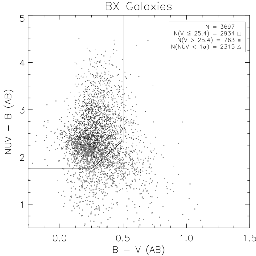
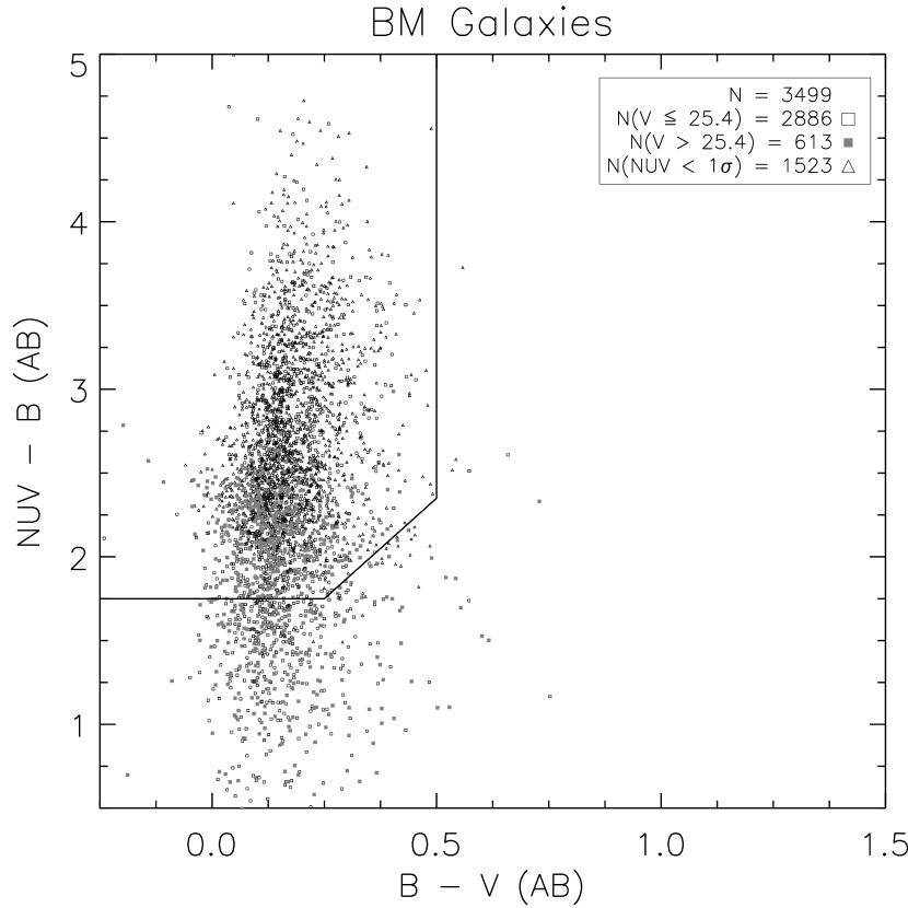
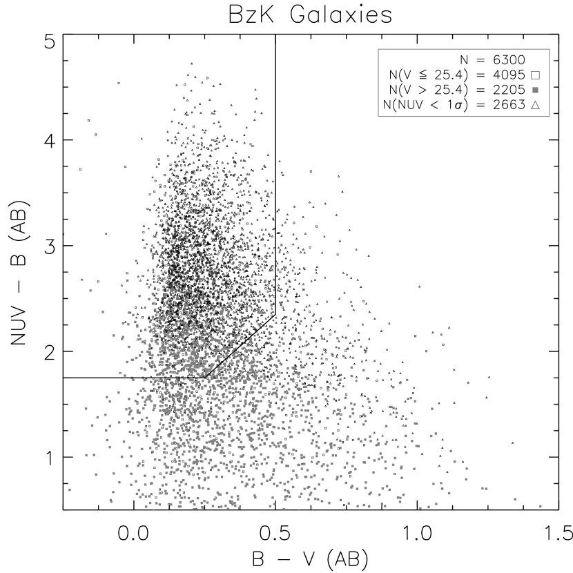
Figure 24.— Sample overlap: $NUV-B$ and $B-V$ colors for BX-, BM-, and BzK-selected galaxies. We have limited these sources to those with $z_{\rm phot}\geq 1.5$ since the NUV data are only able to see the Lyman continuum break at $z\sim 1.5$. Sources below $V=25.4$ are shown as gray squares. Triangles are sources that are undetected in the NUV.

Summary. We find that the overlap fraction between UV- and NIR-selected samples (with typical restrictions on optical and NIR depths) of $z=1$–3 galaxies is high: 74%–98%. The sample overlap was greater when examining the UV-selected samples in the BzK color space rather than vice versa. This illustrates that UV selection techniques, which are good at identifying blue high-$z$ galaxies, miss the redder galaxies, particularly the more massive ones. This has been seen in previous studies (e.g., Q07, ). Several comparisons between the BX/BM galaxies and the $z\sim 2$ LBGs confirm that most (80%–87%) BX/BM galaxies do show a strong Lyman-limit break. This implies that these UV-selected galaxies are nearly analogous to Lyman break selected galaxies. However, the NUV-dropout population does span a wider range in dust extinction, and shows greater overlap with bright sBzK galaxies.

6.3. The Star Formation Rate Density from the Census

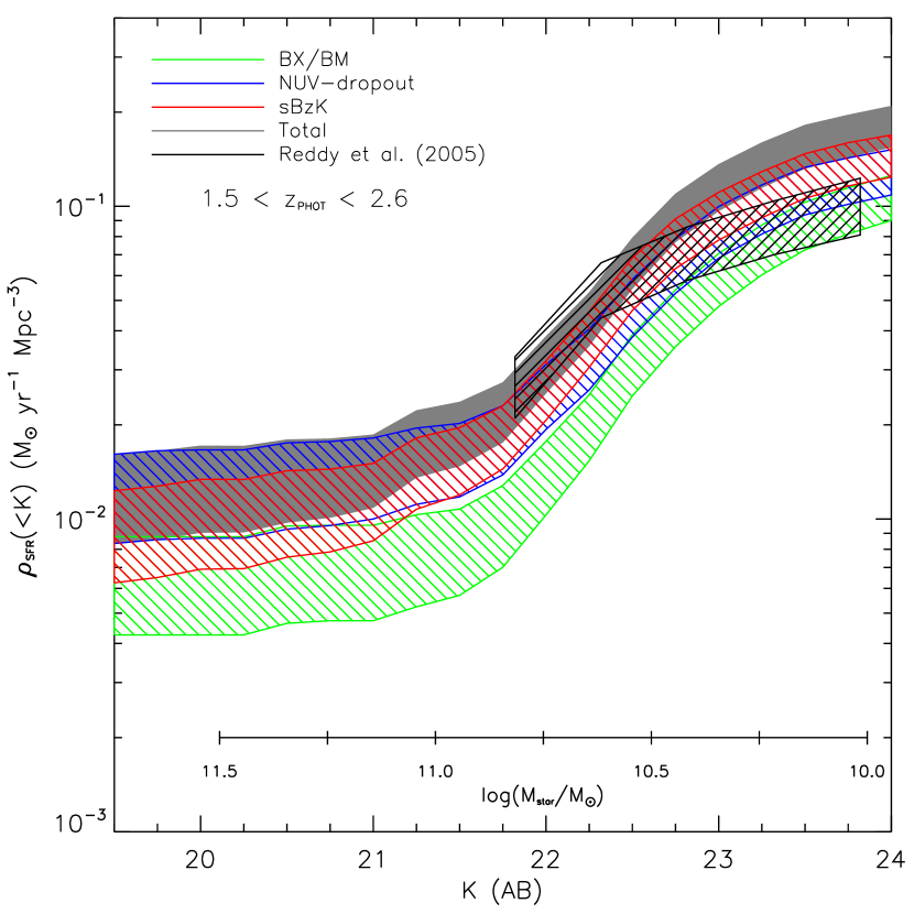
Figure 25.— Accumulated SFR density against $K$- (top) and $R_{\rm C}$-band (bottom) magnitudes from a census of star-forming galaxies at $1.5<z_{\rm phot}<2.6$. Shaded regions include uncertainties in the SFR due to the $z_{\rm phot}$ accuracy and cosmic variance estimates from Somerville et al. (2004). The census total is shown by the shaded gray region while those determined using the sBzK, BX/BM, and NUV-dropout methods are shown by the hatched red, green, and blue regions, respectively. A stellar mass or observed 1700 Å SFR scale is provided for guidance. The stellar mass is from Daddi et al. (2004) SED-fit relation. For the UV SFR, we adopt Kennicutt (1998) relation. (A color version of this figure is available in the online journal.)

With a census of star-forming galaxies from the combined color selection techniques, we can determine the SFR density from the results of our SED modeling with FAST. R05 first estimated this with a census of DRGs, BX and BM galaxies, and sBzK galaxies at $1.4<z_{\rm spec}<2.6$. We consider sBzK, BX and BM, and NUV-dropout galaxies, and limit our sample to $1.5<z_{\rm phot}<2.6$, since this is the overlap range where all three techniques work. While our census does not include DRGs, R05 reported that these galaxies contribute $\lesssim 20\%$ towards the SFR density via their census.

We determine the integrated SFR density as a function of $K$- and $R_{\rm C}$-band magnitudes for the three populations and the full census accounting for sample overlap. To normalize our SFR measurements by the effective survey volume, we assume that the completeness $C(z)$ of the census at any given redshift is proportional to the $z_{\rm phot}$ distribution normalized to unity at the $z_{\rm phot}$ peak. We note that this is a lower limit on incompleteness, so SFR density measurements reported here can be underestimated. The following equation,

$$V_{\rm eff}=\Omega\int_{z=1.5}^{z=2.6}dzC(z)\frac{dV}{dzd\Omega},$$ (13)

yields volumes of $1.18\times 10^{6}$ Mpc³ and $1.24\times 10^{6}$ Mpc³ when we consider sources with $K\lesssim 24$ and $R_{\rm C}\leq 25.5$ mag, respectively. We determined a total SFR density of 0.18$\pm$0.03 (0.18$\pm$0.03) $M_{\sun}$ yr^-1 Mpc^-3 for sources brighter than $K=24.0$ mag ($R_{\rm C}=25.5$ mag). The SFR density is illustrated in Figure 25, where the range of allowed values is $1\sigma$ from including uncertainties in the SFRs due to the $z_{\rm phot}$ accuracy and cosmic variance (estimated from Somerville et al., 2004).

It appears that the SFR density down to a stellar mass limit is mostly contributed by sBzK galaxies. They are not only numerous in the sky, but also have significant star formation that is obscured by dust. For example, while one-fourth of the census is composed of star-forming galaxies with $E(B-V)>0.25$, they account for 65% of the integrated SFR density. If a cut of $E(B-V)=0.4$ mag (recall that the BX/BM and NUV-dropout techniques are sensitive up to $E(B-V)\sim 0.4$ mag) is adopted, then $\approx$64% of the total SFR density is from “less” dusty galaxies.

Compared to R05, we find a higher integrated SFR density by 67%. However, R05 was unable to select NUV-dropouts. Therefore, if we removed galaxies that uniquely meet the NUV-dropout selection, then the SFR density for $K<24.0$ mag is reduced by 10% to 0.16$\pm$0.03 $M_{\sun}$ yr^-1 Mpc^-3, which is still $\sim$50% higher than the reported value of R05.

One explanation for the comparatively higher SFR density is the effect of field-to-field fluctuations on the sBzK galaxy population. In Figure 14, we compared different sBzK surveys and found that the SDF sBzK counts agree well with those from COSMOS (McCracken et al., 2010) down to the COSMOS survey limit of $K\sim 23$. However, R05 begin to see a relative decline at $K\sim 23$ and is approximately a factor of two lower than our measurements at $K\sim 24$. When limited to $z=1.4$–2.6, the surface density reported by R05 is 4.93 arcmin^-2 for $K\lesssim 24$, which is 27% lower when compared to the SDF down to the same limits and redshift range (6.78 arcmin^-2).

To understand the general discrepancy in surface density, we reasoned that field-to-field fluctuations is a likely culprit since R05 covers 72.3 arcmin^-2. As an exercise, we subdivided the SDF into eight independent fields each with the same surveyed area of R05. We determined the surface density as a function of $K$ for each field, and found that the variations observed can fully explain the discrepancy for $K\lesssim 23$ and about half of the differences for $K\sim 23$–24. If this explanation is correct, then such variations can easily affect both the cumulative SFR density from the census of color selection techniques and the contribution to the census solely from sBzK galaxies. For example, among the BX/BM and sBzK census, we find that 66% and 89% are from BX/BM and sBzK galaxies, while R05 report 68% and 67%. In addition, the smaller area coverage of R05 yields a census sample of $\sim$500 galaxies in size, which is statistically less robust when compared to the SDF sample of $\sim$5200 for $z=1.5$–2.6.

6.4. The Completeness of Color Selection Techniques

In Figure 26, we show the redshift distribution for the different color selection techniques and the photo-$z$ sample. For this comparison, we consider photo-$z$ sources that meet the selection depth used for color selections (i.e., 3$\sigma$ detection in $K$, $R_{\rm C}\leq 25.5$ mag, or $V<25.4$ mag). This yields a total of 17566 galaxies with $z_{\rm phot}=1.0$–3.0. It is apparent from Figure 26 that the color selection techniques each identify some subset of galaxies with $z_{\rm phot}=1$–3. We find that the combination of different color selection techniques is able to identify $\approx$90% of galaxies (down to the above magnitude limits) with $z_{\rm phot}=1.5$–2.5. Since the photo-$z$ sample is limited to the depths of the color selection techniques, the missed rate of 10% is likely a result of photometric scatter that drives these galaxies out of the color selection regions.

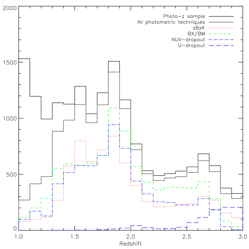
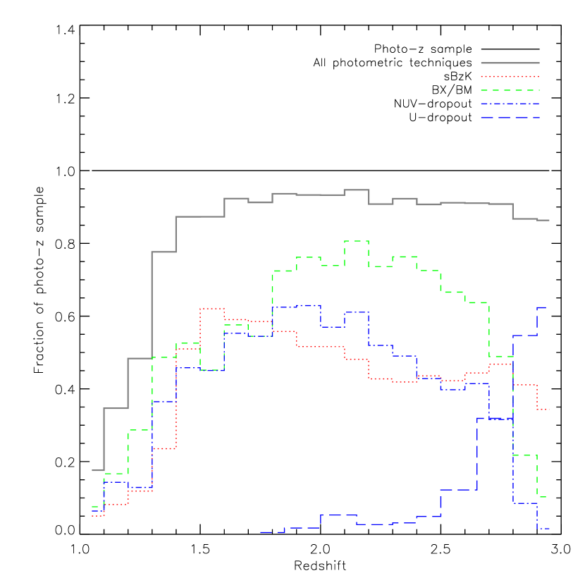
Figure 26.— Comparison between galaxies from color selections and the photo-$z$ sample. The total numbers are shown on the left and the distributions are normalized to the photo-$z$ sample (thin black solid lines) on the right. The sBzK, BX/BM, NUV-dropout, and $U$-dropout samples are indicated by the dotted (red), short-dashed (green), dot-dashed (blue) and long-dashed lines (blue). The combination of these techniques, accounting for overlap between techniques, is shown by the thick gray solid lines. (A color version of this figure is available in the online journal.)

As expected, a noticeable ($\approx$50%) fraction of galaxies with $z_{\rm phot}=1.0$–1.4 are missed. This is because (1) the BzK selection was designed to search at $z\gtrsim 1.5$, (2) two-thirds of the BM galaxy population lie at $z_{\rm phot}>1.5$, (3) almost all BX galaxies are above $z_{\rm phot}>1.5$, and (4) the GALEX/NUV filter only detects a Lyman continuum break at $z_{\rm phot}>1.5$. However, as we discussed previously, recently available Hubble/WFC3 filters are beginning to be used to select galaxies via the Lyman break at $z\sim 1.3$, and such samples may be able to address this loss.

7. Modeled Predictions for a Mock Census

Motivation. To further understand the selection effects of the census derived from color selection techniques (hereafter the “Census”), we generate Monte Carlo realizations of our data and of the Census using mock galaxies that represent the $z\approx 1$–3 population. This simulation intends to (1) examine the stellar population incompleteness effects on the multi-band $\chi^{2}$-weighting scheme (discussed in Section 3.1), (2) create a census of mock LBGs, BX/BM, and BzK galaxies at $z=1.0$–3.5, and (3) compare modeled predictions with observations. In summary, these analyses find both agreements and disagreements with observational results. The former firmly supports many of our main results while the discrepancies appear to have a minor effect.

The ability for a galaxy to be included in the Census is dependent on a few factors. First, galaxies must be identified in the multi-band $\chi^{2}$ image. We required $\chi\geq 3.5$ for at least five connecting pixels. Because the multi-band image spans a wide range in observed wavelengths (4500 Å–2 $\mu$m), these $\chi$ values are influenced by the shape of the SED, which can be parameterized by redshift, stellar mass, dust reddening, galaxy ages, and star formation histories. It is thus important to simulate a wide range of these galaxy properties (see below). Second, we place restrictions on the sample such that they are bright enough to be included in either the 5BK3$\sigma$ or 5B5$\sigma$ photo-$z$ catalogs. Finally, we also apply the different color selection techniques to cull LBGs, BX/BM, and BzK galaxies to generate a “Mock Census.” These steps that we follow are identical to those conducted in Sections 3.1, 4.1, and 5.

Technique/approach. We begin with a grid of spectral synthesis models that adopt a range of magnitudes, redshifts, $E(B-V)$ values, galaxy ages, and $\tau$ values for an exponentially declining star formation history. These models allow us to generate the full SED for artificial galaxies, which are then convolved with the bandpasses for all 15 bands to obtain apparent magnitudes. We then add noise based on known sensitivity at each bandpass to determine the probability of (1) being included into the multi-band $\chi^{2}$ image, (2) satisfying the 5BK3$\sigma$ and/or 5B5$\sigma$ photo-$z$ criteria, and (3) meeting the color selection criteria for the Census.

Assumptions. In estimating the $\chi$ values for mock galaxies, we assume that sources are unresolved with an FWHM of 1$\farcs$1. This process involves normalizing a Gaussian PSF by the S/N of the source in each band, and then taking the square-root of the sum of the squares for eight bands ($BVR_{\rm C}i\arcmin z\arcmin K$, IA598, and IA679). We then determine if the number of connecting 0$\farcs$2 pixels that meets the minimum $\chi=3.5$ criteria is at least five to be included.

The grid of models spans redshifts from 1.0 to 3.2 (0.2 increments), $E(B-V)=0.0$–0.5 (0.1 increments), and ages between $\log({\rm age/yr})=7.0$ dex and the age of the universe at a given redshift (0.25 dex increments). We adopt exponentially declining star formation history with $\tau$ = 0.1, 1.0, and 10.0 Gyr. The limits on these properties are identical to those assumed in modeling the SEDs (see Section 4.2). We also assume a Chabrier (2003) IMF and solar metallicity for the spectral synthesis models. We also include redshift-dependent IGM absorption from neutral hydrogen for rest wavelengths blueward of 1216 Å following Madau (1995). With these parameters, we have a total of 2,268 SEDs. These SEDs are normalized in the $z$′-band between 20.0 and 26.0 mag (0.5 mag increments), which yields 27,216 possible models. We chose to normalize at $z$′ since it is the most sensitive band closest to $K$. The use of the $z$′-band also provides a good compromise between the rest-frame UV (sensitive to recent star formation) and optical (sensitive to stellar mass).

We must adopt distributions for each modeled properties (e.g., $E(B-V)$, redshift, and magnitude). First, we assume that the observed $z\sim 1$–3 $E(B-V)$ distribution applies to all galaxies in the simulation. This simplifying assumption is needed for a proper normalization of the number of blue-to-red galaxies, since it will affect the overlap fraction between sBzK and BX/BM or LBGs and the fraction of the Census that is contributed by either method. The $E(B-V)$ distribution shows a log-normal decline with higher dust reddening following $\log{(N)}\propto-3.3\times E(B-V)$. Then for each $E(B-V)$ bin, we use observational constraints on the redshift and magnitude distributions. The observed distributions show that the more reddened galaxies are found at $z\lesssim 2$ and have brighter $z$′ magnitudes (see Figure 27). In total, we generate 34,755 mock galaxies and the simulation is repeated 100 times for 3,475,500 artificial galaxies.

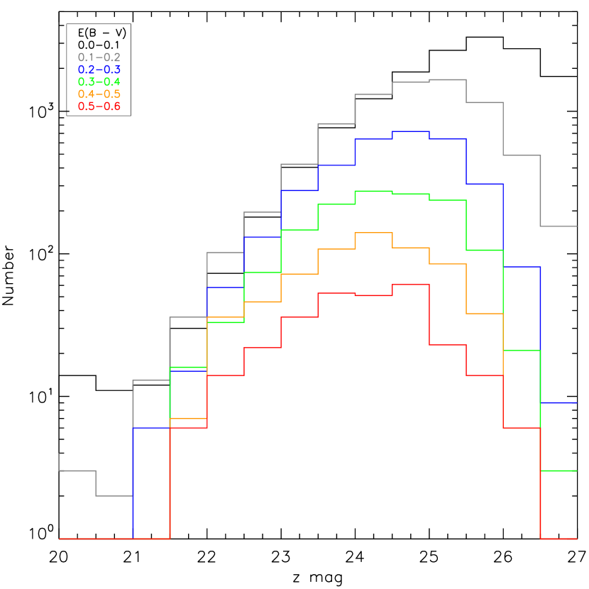
Figure 27.— Redshift (left) and $z$′-band (right) distributions for galaxies with different measured $E(B-V)$. These distributions are used as prior inputs for the Monte Carlo simulation. This figure illustrates that (observationally) most of the dusty galaxies are found at $z\lesssim 2$ and at relatively brighter $z$′ magnitudes. (A color version of this figure is available in the online journal.)

One caveat with these assumptions is that observed trends and distributions are used, which themselves are affected by incompleteness. For example, we could be underestimating the intrinsic number of extremely dusty and/or old galaxies. However, neither we nor previous investigators have sufficient information to attempt a further correction for this possible incompleteness.

Predictions from simulations. With the Monte Carlo realization of our data, we find that the $\chi^{2}$ method begins to miss 5% (50%) of galaxies at $V\approx 26.25$ ($V\approx 27.25$) and $R_{\rm C}\approx 25.75$ ($R_{\rm C}\approx 26.5$). This simulation shows that the $\chi^{2}$ method is highly complete down to magnitudes, $V=25.4$ and $R_{\rm C}=25.5$, at which we select NUV-dropouts and BX/BM galaxies using optical colors.

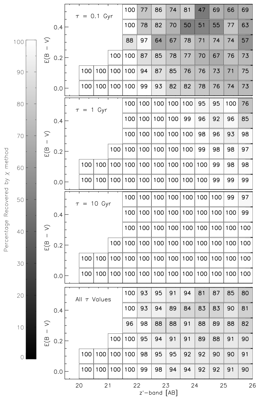
Figure 28.— Recovered fraction of mock galaxies as a function of the assumed star formation history, dust reddening, and magnitude. Each panel plots $E(B-V)$ as a function of $z$′. Results for $\tau=0.1$, 1, and 10 Gyr and all three combined are shown from top to bottom. The gray scale shows the completeness from 100% (white) to 0% (black). Faint magnitude bins with high reddening have large statistical fluctuations due to input small numbers.

In Figure 28, we illustrate the fraction recovered by the $\chi$ method as a function of dust reddening and the $z$′-band magnitude for the different $\tau$ models. This figure illustrates high ($\gtrsim$80%) completeness for the $\tau=1$ and 10 Gyr models regardless of brightness and $E(B-V)$. As expected, the model with the shortest timescale for star formation will suffer more incompleteness since many of these galaxies are evolved and dust reddening further hampers their inclusion in the $\chi^{2}$ image. By coming all three $\tau$ models, the incompleteness does not exceed 20%.

Comparisons with observations. In addition to the above completeness estimates, our Monte Carlo simulation provides a few commensurable predictions. For example, in Figure 29 we illustrate the fraction of the Mock and Observed Census that is probed by each color selection technique. This is similar to Figure 18 but with fixed redshift bins. There are several similarities that are apparent. The simulated $U$-dropout and BX distributions are fairly consistent with observations in the terms of the location and strength of the peak and the shape of the distributions. The sBzK distributions peak at $z\sim 1.5$ at 80% (mock) and 70% (observed) and declines to 30%–40% at $z\gtrsim 3$. Above $z=1.7$, the $z\sim 2$ LBG distributions are similar peaking at $z\sim 2$ and extending out to $z\sim 2.8$. These similarities strongly suggest that the overlap determined between each population is a fairly reliable result, and it is indeed true that no technique yields 100% of the Census at any redshift. The greatest discrepancy, is at $z\lesssim 1.5$ where the mock simulation indicates higher completeness. The causes for such discrepancies is not known. However, these differences do not affect much of our main results which concern $z\gtrsim 1.5$.

Figure 29.— Comparison between the Mock Census (left) and the observed Census (right). The vertical axes show the fraction of the Census consisting of LBGs (black), BX (green), BM (blue), and sBzK (red) galaxies. These plots are a reproduction of Figure 18. Our Mock Census is able to reproduce the redshift peak of each galaxy population and the shape of the redshift distributions above $z\sim 1.5$. These comparisons are further discussed in Section 7. (A color version of this figure is available in the online journal.)

Another prediction from the simulation is the fraction of the photo-$z$ census that is recovered by the Census (see Figure 30). As we have shown, the observed census yields 90% of galaxies above $z=1.5$, and this appears to hold out to $z\sim 3$. The Mock Census shows a similar behavior, but indicates nearly 100%. These differences are small since Poisson statistics is at the $\sim$5% level.

Figure 30.— Comparison between the Mock Census (solid line) and the observed Census (dashed line). The vertical axis shows the fraction of the photo-$z$ sample that consists of galaxies that satisfy either one of the criteria for being BX, BM, sBzK  and LBGs at $z\sim 2$ and $z\sim 3$. This is a reproduction of Figure 26 (right). The Mock Census yields a higher fraction than observed; however, it is consistent to within 2$\sigma$ of Poisson statistics. These comparisons are further discussed in Section 7.

Finally, another set of positive comparisons is the $V$-, $R_{\rm C}$-, and $K$-band luminosity functions for $z\sim 2$ LBGs. We find good to reasonable agreement over 5 magnitudes in the optical bands and 3 magnitudes in $K$. Other color selection techniques find agreements over a smaller range of magnitudes. The causes of poorer agreement are still unknown.

8. Conclusions

We have conducted a large photometric survey of galaxies at $z=1$–3 by synthesizing measurements from 20 broad-, intermediate-, and narrow-band filters covering observed wavelengths of 1500 Å–4.5 $\mu$m. This survey is unique due to its size (0.25 deg²; $5.6\times 10^{6}$ Mpc³ for $z=1$–3), depth, and reliable photo-$z$’s derived for $\approx$23,000 $K$-band selected sources ($\approx$65,000 including optically selected sources). Compared to a spectroscopic sample, we find that our photo-$z$’s from 20-bands are accurate to $1.2\%\times(1+z)$ (1$\sigma$) for $z\lesssim 1.8$. The accuracy of our photo-$z$ stems from coverage of both the Lyman continuum and Balmer/4000 Å breaks at $z\sim 2$ with the multiple bands that we have. Most photo-$z$ surveys use 10 photometric bands or less, are limited to accurate redshifts below $z\lesssim 1$ and $z\gtrsim 3$, and suffer from a common photo-$z$ problem of ambiguity between the Balmer/4000 Å break at $z\sim 0.3$ and Lyman break at $z\sim 3$.

We have also examined the $z_{\rm phot}$ for $\approx$4500 narrow-band excess emitters at $z\approx 0.25$–1.5, and found excellent to adequate agreement between our derived $z_{\rm phot}$, and the predictions from using simple multiple rest-frame optical colors (see Ly et al., 2007). This evidence further indicates that the photo-$z$ that we have generated are reliable.

In addition, the combination of deep optical and relatively deep NIR data provides a large and representative sample of $z=1$–3 galaxies covering a wide range in stellar mass, dust content, and SFR. With $\approx$21,000 ($\approx$19,000 with $z_{\rm phot}$) galaxies, we are able to study statistically the overlap of different galaxy populations (BX/BM, LBG, and BzK) obtained from each technique. We also investigate the completeness of these techniques against a sample derived purely from photo-$z$. The main results for this paper are:
Redshift distribution. We determined (with accurate photo-$z$) that 74.7% of BXs, 84.5% of BMs, 78.83% of $U$-dropouts, 93.9% of sBzKs, and 91.9% of NUV-dropouts have $z_{\rm phot}=1$–3.5. We find that the BX, BM, and $U$-dropout methods suffer from $z_{\rm phot}<0.5$ contamination at the 24.4%, 12.8%, and 13.4% levels, respectively. This problem is largely attributed to the Balmer/4000 Å break occurring between the $U$ and $B$ filters, rather than a Lyman break. We also find that the NUV-dropout technique has 17.4% contamination from “interlopers” at $z=1.0$–1.5, which eliminates a previous concern that contamination fraction estimates in Ly et al. (2009) were too optimistic. Also, the technique does not suffer from $z<0.5$ interlopers, since the Balmer break is redward of the NUV.

Selection bias and completeness of techniques. We confirmed that each color selection is biased towards some subset of galaxies not fully representative of the entire galaxy population. By modeling the SED of thousands of photometrically-selected galaxies, we find that the BzK method targets more massive and dusty galaxies, while the BX, BM, and $U$-dropout methods identify galaxies of lower stellar mass with low reddening. Compared to a combined census of color-selected galaxies (BX/BM, LBG, and BzK), we find that any UV or IR technique finds at most 60%–80% at the peak of their redshift sensitivity. However, these techniques are optimized for a certain redshift range, so relative to a $z=1$–3 color-selected census, the BX/BM, NUV-dropout and sBzK techniques obtain 52%–65%. This strongly indicates that combining multiple techniques is favored for a complete census of high-redshift galaxies and their SFRs. We estimate that the BX/BM method is capable of identifying (by number) 70% of $z_{\rm phot}=1$–3 census galaxies with SFR between a few and 30 $M_{\sun}$ yr^-1, and this represents 66% of the $z_{\rm phot}=1$–3 census.

Sample overlap between galaxy populations. Among the star-forming BzK-selected galaxies, the overlap fraction with the BX/BM/$U$-dropout increases at fainter $K$ luminosities, consistent with R05. However, with a larger sample of massive sBzK galaxies, we determined that the overlap fraction is $\sim$5 times smaller than what was reported in R05 at bright $K$ magnitudes. We argue that this is due to the smaller FoV and sample size that they used. Our study also shows that 77.2% of $z\geq 1.5$ sBzK galaxies have a strong Lyman break to meet the NUV-dropout criteria. Unlike the BX/BM method, this overlap fraction is independent of $K$ mag, indicating that the Lyman break technique is relatively more sensitive to massive galaxies. Likewise, we find that 79.7% of $z\geq 1.5$ BX and 87.0% of $z\geq 1.5$ BM galaxies are $z\sim 2$ LBGs. These results indicate that the 912 Å break is ubiquitous in $z\sim 2$ galaxies. Thus, the NUV-dropout selection differs from the BX/BM selection by including more massive and reddened galaxies.

SFR density from a census of UV- and NIR-selected galaxies. We determined that the comoving SFR density at $z_{\rm phot}=1.5$–2.6 is 0.18$\pm$0.03 $M_{\sun}$ yr^-1 Mpc^-3 from a joint census of BzK galaxies, BX/BM galaxies, and LBGs. This census was limited to galaxies with $K\lesssim 24$ (corresponds to $\approx 10^{10}$ $M_{\sun}$). We find that the UV selection methods (Lyman break and BX/BM) obtain 81% of the SFR density from galaxies with $E(B-V)<0.25$ mag. These low reddening galaxies represent about three-quarters of our census by number. However, there is a prominent population of galaxies with high dust extinction ($E(B-V)>0.25$ mag). For example, we examined the contribution to the SFR density relative to the dust properties of our galaxies, and find that galaxies below and above $E(B-V)=0.25$ mag contribute 35% and 65% to the SFR density, respectively.

Completeness of color selection techniques. We compare the census derived from color selection techniques against a photo-$z$ sample, and find that color selection is (1) less efficient at $z\lesssim 1.5$, but (2) identifies $\approx$90% of galaxies at $z_{\rm phot}=1.5$–2.5. We also find that the sBzK method is 85% complete when compared against a sample of $K$-band detected sources with $z_{\rm phot}>1.5$. This evidence, combined with the high fraction of overlap between BX/BM and sBzK galaxies for $K\sim 23$–24 AB mag, and the likelihood that faint (blue) UV-selected galaxies will be detected with deeper $K$-band imaging, strongly suggest that future $z\approx 1$–3 studies should focus on a very deep $K$-band imaging (e.g., the Ultra-VISTA survey). But until such a deep ($K\sim 25$–26 AB) survey with multi-wavelength data is available over large areas, the UV selection techniques (either the $U_{n}G\mathcal{R}$ or NUV-dropout method) are currently the only efficient way to identify less massive $z\sim 2$ galaxies.

Appendix A Unusual Sources from Color Selection

About half of the Shallow and Faint samples (restricted to the deep $K$-band area and excluding galaxies with $z_{\rm phot}<0.5$) consists of sources that are uniquely selected by only one color selection. These sources are of great interest, since they indicate that a particular technique culls a galaxy sample that is unavailable by any other techniques. We summarize the uniqueness below.
Passive BzK galaxies. We find that the entire pBzK sample does not overlap with any of the other techniques. These galaxies at $z\approx 1$–2 have the oldest ages, $\log{(t_{\rm age}/{\rm yr})\approx 9.0}$, the highest stellar masses, $\log{(M/M_{\sun})\approx 11.0}$, and span $E(B-V)=0.0$–0.3. Their ages imply that they formed $\Delta z=0.6$ earlier (median formation redshift is $z=2.25$), and could be the descendants of luminous infrared galaxies or massive LBGs with SFRs $\gtrsim 100$ $M_{\sun}$ yr^-1. These galaxies are important for a stellar mass census survey, but contribute little to the SFR density since their SFRs are on average 0.02 $M_{\sun}$ yr^-1.
Star-forming BzK galaxies. We find that purely sBzKs, compared to UV-selected samples, have similar SFRs ($\sim 5$ $M_{\sun}$ yr^-1), but are more massive ($\sim 10^{9.5}$–$10^{11}$ $M_{\sun}$), cover a broader range in dust extinction ($E[B-V]\approx 0.05$–0.4), and are 0.5 dex older.
BX, BM, and $U$-dropout galaxies. The UV selection techniques of Steidel et al. identify a unique set of galaxies with relatively younger stellar ages (typically $2\times 10^{8}$ yr), lower stellar mass ($\sim 10^{9}$ $M_{\sun}$), and $E(B-V)\approx 0.1$. We find that the SFRs are systematically lower by 0.2–0.3 dex for BM and BX galaxies when compared to $U$-dropouts, although this is likely a manifestation of redshift dependence of the sample. The relatively poor $U$-dropout overlap with NIR techniques can be attributed to the redshift of the sample, as well as, the lack of deeper NIR data. It would be prudent to identify a sample of higher redshift BzK galaxies using a set of different filters (e.g., $R$, $J$, and $L$; Daddi et al., 2004) to investigate the overlap of LBGs at higher redshift with 3.6 $\mu$m-selected galaxies.
Lyman break galaxies at $z\sim 2$. The method that we developed to identify LBGs at $z\approx 1.5$–2.5 has significant overlap ($\approx$80%) with the BX/BM and/or BzK techniques. It appears that the remaining 20% consists of galaxies with stellar masses of $\approx 10^{10\pm 1}$ $M_{\sun}$, cover the same stellar ages as other techniques, have an average SFR of $\sim$20 $M_{\sun}$ yr^-1, and span $E(B-V)=0.1$–0.4. The main reason for why these galaxies were uniquely identified is their redshift: about two-thirds of them are below $z=1.5$ where the sBzK and BM techniques are less sensitive. We note that the higher SFRs for NUV-dropouts are likely due to the limit adopted for the $V$-band (our limit is comparable brighter than $R_{\rm C}=25.5$ for BX/BM). The fainter ($V=26.0$) limit yields an average SFR that is systematically lower by 0.2 dex, due to the higher contribution from lower-SFR LBGs.

References

- Adelberger et al. (2004) Adelberger, K. L., Steidel, C. C., Shapley, A. E., Hunt, M. P., Erb, D. K., Reddy, N. A., & Pettini, M. 2004, ApJ, 607, 226
- Baum (1962) Baum, W. A. 1962, in Proc. IAU Symp. 15, Problems of Extra-Galactic Research, ed. G. C. McVittie (Cambridge: Cambridge Univ. Press), 390
- Bertin & Arnouts (1996) Bertin, E., & Arnouts, S. 1996, A&AS, 117, 393
- Bolzonella et al. (2000) Bolzonella, M., Miralles, J.-M., & Pelló, R. 2000, A&A, 363, 476
- Bouwens et al. (2006) Bouwens, R. J., Illingworth, G. D., Blakeslee, J. P., & Franx, M. 2006, ApJ, 653, 53
- Brammer et al. (2008) Brammer, G. B., van Dokkum, P. G., & Coppi, P. 2008, ApJ, 686, 1503
- Bruzual & Charlot (2003) Bruzual, G., & Charlot, S. 2003, MNRAS, 344, 1000
- Burgarella et al. (2007) Burgarella, D., et al. 2007, MNRAS, 380, 986
- Calzetti et al. (2000) Calzetti, D., Armus, L., Bohlin, R. C., Kinney, A. L., Koornneef, J., & Storchi-Bergmann, T. 2000, ApJ, 533, 682
- Casali et al. (2007) Casali, M., et al. 2007, A&A, 467, 777
- Chabrier (2003) Chabrier, G. 2003, PASP, 115, 763
- Daddi et al. (2004) Daddi, E., Cimatti, A., Renzini, A., Fontana, A., Mignoli, M., Pozzetti, L., Tozzi, P., & Zamorani, G. 2004, ApJ, 617, 746
- Franx et al. (2003) Franx, M., et al. 2003, ApJ, 587, L79
- Grazian et al. (2007) Grazian, A., et al. 2007, A&A, 465, 393 [G07]
- Hathi et al. (2010) Hathi, N. P., et al. 2010, ApJ, 720, 1708
- Hayashi et al. (2007) Hayashi, M., Shimasaku, K., Motohara, K., Yoshida, M., Okamura, S., & Kashikawa, N. 2007, ApJ, 660, 72
- Ilbert et al. (2009) Ilbert, O., et al. 2009, ApJ, 690, 1236
- Kashikawa et al. (2004) Kashikawa, N., et al. 2004, PASJ, 56, 1011
- Kashikawa et al. (2006) Kashikawa, N., et al. 2006, ApJ, 648, 7
- Kennicutt (1998) Kennicutt, R. C. 1998, ARA&A, 36, 189
- Kong et al. (2006) Kong, X., et al. 2006, ApJ, 638, 72
- Kriek et al. (2009) Kriek, M., van Dokkum, P. G., Labbé, I., Franx, M., Illingworth, G. D., Marchesini, D., & Quadri, R. F. 2009, ApJ, 700, 221
- Landolt (1992) Landolt, A. U. 1992, AJ, 104, 340
- Lane et al. (2007) Lane, K. P., et al. 2007, MNRAS, 379, L25 [L07]
- Ly et al. (2007) Ly, C., et al. 2007, ApJ, 657, 738
- Ly et al. (2009) Ly, C., et al. 2009, ApJ, 697, 1410 [L09]
- Madau (1995) Madau, P. 1995, ApJ, 441, 18
- Malkan (2004) Malkan, M. 2004, Galex Cycle 1, Proposal 65
- Malkan et al. (2005) Malkan, M., Iye, M., Kashikawa, N., Kodama, T., Motohara, K., & Shimasaku, K. 2005, Spitzer Proposal ID 20229
- Maraston (2005) Maraston, C. 2005, MNRAS, 362, 799
- Martin et al. (2005) Martin, D. C., et al. 2005, ApJ, 619, L1
- McCracken et al. (2010) McCracken, H. J., et al. 2010, ApJ, 708, 202
- Meisenheimer & Wolf (2002) Meisenheimer, K., & Wolf, C. 2002, Astron. Geophys., 43, 15
- Miyazaki et al. (2002) Miyazaki, S., et al. 2002, PASJ, 54, 833
- Muller et al. (1998) Muller, G. P., Reed, R., Armandroff, T., Boroson, T. A., & Jacoby, G. H. 1998, Proc. SPIE, 3355, 577
- Nagao et al. (2008) Nagao, T., et al. 2008, ApJ, 680, 100
- Oke (1974) Oke, J. B. 1974, ApJS, 27, 21
- Ouchi et al. (2003) Ouchi, M., et al. 2003, ApJ, 582, 60
- Probst et al. (2008) Probst, R. G., George, J. R., Daly, P. N., Don, K., & Ellis, M. 2008, Proc. SPIE, 7014, 70142S
- Probst et al. (2004) Probst, R. G., et al. 2004, Proc. SPIE, 5492, 1716
- Quadri et al. (2007) Quadri, R., et al. 2007, AJ, 134, 1103 [Q07]
- Reddy et al. (2005) Reddy, N. A., Erb, D. K., Steidel, C. C., Shapley, A. E., Adelberger, K. L., & Pettini, M. 2005, ApJ, 633, 748 [R05]
- Reddy et al. (2008) Reddy, N. A., Steidel, C. C., Pettini, M., Adelberger, K. L., Shapley, A. E., Erb, D. K., & Dickinson, M. 2008, ApJS, 175, 48
- Salpeter (1955) Salpeter, E. E. 1955, ApJ, 121, 161
- Shimasaku et al. (2005) Shimasaku, K., Ouchi, M., Furusawa, H., Yoshida, M., Kashikawa, N., & Okamura, S. 2005, PASJ, 57, 447
- Shimasaku et al. (2003) Shimasaku, K., et al. 2003, ApJ, 586, L111
- Shimasaku et al. (2004) Shimasaku, K., et al. 2004, ApJ, 605, L93
- Shimasaku et al. (2006) Shimasaku, K., et al. 2006, PASJ, 58, 313
- Skrutskie et al. (2006) Skrutskie, M. F., et al. 2006, AJ, 131, 1163
- Somerville et al. (2004) Somerville, R. S., Lee, K., Ferguson, H. C., Gardner, J. P., Moustakas, L. A., & Giavalisco, M. 2004, ApJ, 600, L171
- Steidel et al. (1999) Steidel, C. C., Adelberger, K. L., Giavalisco, M., Dickinson, M., & Pettini, M. 1999, ApJ, 519, 1
- Steidel et al. (2003) Steidel, C. C., Adelberger, K. L., Shapley, A. E., Pettini, M., Dickinson, M., & Giavalisco, M. 2003, ApJ, 592, 728
- Steidel et al. (2004) Steidel, C. C., Shapley, A. E., Pettini, M., Adelberger, K. L., Erb, D. K., Reddy, N. A., & Hunt, M. P. 2004, ApJ, 604, 534 [S04]
- Szalay et al. (1999) Szalay, A. S., Connolly, A. J., & Szokoly, G. P. 1999, AJ, 117, 68
- van Dokkum et al. (2004) van Dokkum, P. G., et al. 2004, ApJ, 611, 703
- van Dokkum et al. (2009) van Dokkum, P. G., et al. 2009, PASP, 121, 2
- Velusamy et al. (2008) Velusamy, T., Marsh, K. A., Beichman, C. A., Backus, C. R., & Thompson, T. J. 2008, AJ, 136, 197
- Yoshida et al. (2006) Yoshida, M., et al. 2006, ApJ, 653, 988