Bubble doubling route to strange nonchaotic attractor
in a quasiperiodically forced Chua’s circuit

Abstract

We have identified a novel mechanism for the birth of Strange Nonchaotic Attractor (SNA) in a quasiperiodically forced Chua’s circuit. In this study the amplitude of one of the external driving forces is considered as the control parameter. By varying this control parameter, we find that bubbles appear in the strands of the torus. These bubbles start to double in number as the control parameter is increased. On increasing the parameter continuously, successive doubling of the bubbles occurs, leading to the birth of SNAs. We call this mechanism as the bubble doubling mechanism. The formation of SNA through this bubble doubling route is confirmed numerically, using Poincaré maps, maximal Lyapunov exponent and its variance and the distribution of finite-time Lyapunov exponents. Also a quantitative confirmation of the strange nonchaotic dynamics is carried out with the help of singular continuous spectrum analysis.

I Introduction

Strange Nonchaotic Attractors (SNAs) are known to appear in quasiperiodically forced dynamical systems. They posseses a complicated geometrical structure, which shows them to be fractal in nature, but do not have any sensitive dependence on initial conditions, as seen from a negative maximal Lyapunov exponent. Following the pioneering work by Grebogi et al. greb , many researchers have found the existence of the SNAs, and have even classified the mechanisms for their occurrence in quasiperiodically forced continuous dynamical systems and maps. In particular the SNAs have been reported to arise in many physically relevant situations such as the quasiperiodically forced pendulum rome , the quantum particles in quasiperiodic potentials bond , biological oscillators ding , the quasiperiodically driven Duffing-type oscillators venk ; heag ; yalc ; kapi ; feud , velocity dependent oscillators venk1 , electronic circuits yang ; zhiw ; venk2 , and in certain maps pras ; piko ; piko1 ; kuzn ; anis ; nish ; venk3 ; hunt ; kim ; lim ; heag1 . Also, these exotic attractors were confirmed by an experiment consisting of a quasiperiodically forced, buckled, magnetoelastic ribbon ditt , in analog simulations of a multistable potential zhou , and in a neon glow discharge experiment ding1 . The SNAs are also related to the Anderson localization in the Schrödinger equation with a quasiperiodic potential keto ; pras1 and they may have a practical application in secure communication zhou1 ; rama1 ; chac .

Broadly the mechanisms for the birth of SNAs differ with the routes to SNA followed by the dynamical systems. A list of the various mechanisms pertaining to different routes to chaos are listed in Table - I pras2 . Very recently, a new route namely the bubble route to SNAs have been reported by Senthilkumar et al. sent in a quasiperiodically forced negative conductance series $LCR$ circuit with a diode, wherein, one of the driving force is a non-sinusoidal (square wave). In this route bubbles appear in the strands of the torus as a function of the control parameter. These bubbles then grow in size as the control parameter is increased. Subsequently the strands of the bubbles start to wrinkle, giving birth to SNAs. The reason for this is that the quasiperiodic orbits become increasingly unstable in the transverse direction with the increase of the control parameter. This instability is induced by the square wave type quasiperiodic force resulting in an increase in the size of the doubled strands (bubbles), followed by an enhanced wrinkling of these.

Table 1: Routes and mechanisms for the formation of SNAs

Type of route	Mechanism
Heagy-Hammel heag1	Collision of period-doubled torus with its unstable parent
Gradual Fractilization nish	Increased wrinkling of torus without any interaction with nearby periodic orbits
On-off intermittency yalc	Loss of transverse stability of torus
Type-I intermittency pras	Due to saddle-node bifurcation, a torus is replaced by SNA
Type-III intermittency venk2	Subharmonic instability
Homoclinic collision pras1	Homoclinic collisions of the quasiperiodic orbits

In this present work, we report successively doubling of the bubbles route to SNAs in a quasiperiodically forced Chua’s circuit. Here, the bubbles appear in the strands of the torus as a function of the control parameter, then grow in size and get doubled in number. After many successive doubling of the bubbles, SNAs are born. All through these, the remaining part of the strands of the torus which do not contain the bubbles, remain unaffected even though varying the control parameter. In this route no wrinkling of the bubbles are found to occur sent . In order to confirm this, we present here a detailed numerical analysis using Poincaré map, Fourier spectrum, maximal Lyapunov exponent, its variance, finite time Lyapunov exponents and separation of near by trajectories in phase space. Further the singular continuous spectrum analysis is used to find scaling the exponent and fractal paths.

The paper is organized as follows. In Sec. II, we discuss the circuit realization of the quasiperiodically forced Chua’s circuit. In Sec. III, the observations of the bubble doubling route to SNAs are given with the help of Poincaré cross section. In Sec. IV, we substantiate the observations by the maximal Lyapunov exponent spectrum and its variance. In Sec. V, we find the scaling exponent and fractal path by using singular continuous spectrum analysis. In Sec. VI, we discuss another qualitative measure of this route by separation of near by trajectories. In Sec. VII, the finite time Lyapunov exponents are used to confirm the SNA and show the mechanism of the bubble doubling route. Finally, in Sec. VIII, we summarize our results.

II Circuit Realization

The quasiperiodically forced Chua’s circuit zhiw is shown in Fig. (1). Using Kirchoff’s laws, the equations of this circuit derived are

$$C_{1}\frac{dv_{C_{1}}}{dt} = G(v_{C_{2}}-v_{C_{1}})-g(v_{C_{1}}),$$ (1a)

$$C_{2}\frac{dv_{C_{2}}}{dt} = G(v_{C_{1}}-v_{C_{2}})+i_{L},$$ (1b)

$$L\frac{di_{L}}{dt} = -v_{C_{2}}+F_{1}\sin(\omega_{1}t)+F_{2}\sin(\omega_{2}t).$$ (1c)

Here,

$$g(v_{C_{1}})=G_{b}v_{C_{1}}+0.5(G_{a}-G_{b})[|v_{C_{1}}+B_{p}|-|v_{C_{1}}-B_{p}|]$$ (1d)

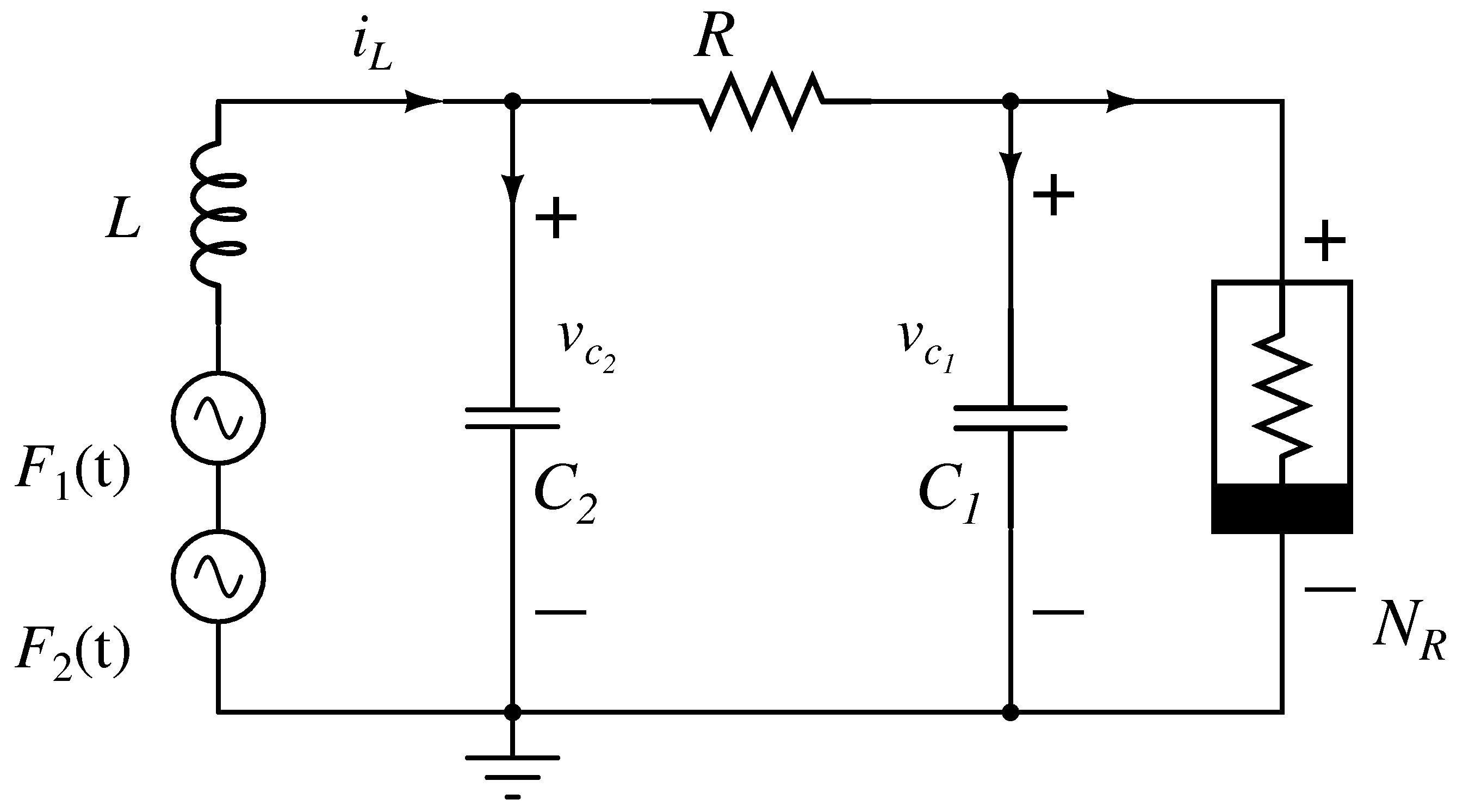
Figure 1: ircuit realization of the quasiperiodically forced Chua’s circuit. Here $N_{R}$ is the Chua’s diode. The parameter values of the circuit elements are fixed as $C_{1}=16.8$ nF, $C_{2}=98.0$ nF, $L=18.75$ mH, $R=1565$ $\Omega$ , $G_{a}=-0.758$ mS, $G_{b}=-0.409$ mS, ${\nu_{1}}=2849.0$ Hz, ${\nu_{2}}=3560.0$ Hz and $F_{2}=5$ mV are chosen respectively. The forcing amplitude $F_{1}$ is taken as control parameter which being varied in our analysis.

where $v_{C_{1}}$, $v_{C_{2}}$ are the voltages across the capacitors $C_{1}$ and $C_{2}$, and $i_{L}$ is the current through inductor $L$ respectively. $F_{1}\sin(\omega_{1}t)$ and $F_{2}\sin(\omega_{2}t)$ are the external excitations having incommensurate frequencies, $g(v_{C_{1}})$ is mathematical expression of Chua’s diode. where $G_{b}$ is the outer slope and $G_{a}$ is the inner slope of the nonlinear curve. $B_{P}$ is the break point voltage. The parameter values of the circuit elements are fixed as $C_{1}=16.8$ nF, $C_{2}=98.0$ nF, $L=18.75$ mH, $R=1565$ $\Omega$, $G_{a}=-0.758$ mS and $G_{b}=-0.409$ mS. The value of the $\nu_{1}(=\omega_{1}/2\pi)$ and $\nu_{2}(=\omega_{2}/2\pi)$ are chosen as $2849.0$ Hz and $3560.0$ Hz respectively. The forcing amplitude $F_{2}$ is fixed as 5 mV and the forcing amplitude $F_{1}$ is assumed as the control parameter. In order to study the dynamics of the circuit, the circuit Eqs. (1) can be normalized using the following rescale variables and parameters. $v_{C_{1}}$ $=$ $xB_{p}$, $v_{C_{2}}$ $=$ $yB_{p}$, $i_{L}$ $=$ $B_{p}Gz$, $t$ $=$ $C_{2}\tau/G$, $G$ $=$ $1/R$, $a$ $=$ $RG_{a}$, $b$ $=$ $RG_{b}$, $\alpha$ $=$ $C_{2}/C_{1}$, $\beta$ $=$ $C_{2}R^{2}/L$, $f_{1}$ $=$ $F_{1}\beta/B_{p}$, $f_{2}$ $=$ $F_{2}\beta/B_{p}$, $\omega_{1}$ $=$ $G\Omega_{1}/C_{2}$ and $\omega_{2}$ $=$ $G\Omega_{2}/C_{2}$.

$$\frac{dx}{dt} = \alpha(y-x-h(x)),$$ (2a)

$$\frac{dy}{dt} = x-y+z,$$ (2b)

$$\frac{dz}{dt} = -\beta y+f_{1}\sin(\Omega_{1}t)+f_{2}\sin(\Omega_{2}t),$$ (2c)

where,

$$h(x)=bx+0.5(a-b)[|x+1|-|x-1|].$$ (2d)

Eqs. (2) are numerically integrated using Runge - Kutta fourth order algorithm with step size 0.0001. The values of the normalized parameters are $a$ $=$ $-1.1862$, $b$ $=$ $-0.6400$, $\alpha$ $=$ $5.8333$, $\beta$ $=$ $12.8012$, $\Omega_{1}$ $=$ $2.7454$, $\Omega_{2}$ $=$ $3.4306$ and $f_{2}$ $=$ $0.1280$. The normalized parameter $f_{1}$ of external quasiperiodic forcing is taken as control parameter.

III Bubble Doubling Route to SNA

To observe the emergence of SNA the amplitude of the external forcing $f_{1}$ is varied in the range $f_{1}\in(0.7296,0.8500)$. The Poincaré surface of section plot of the two strands corresponding to period$-$2 torus for the value of $f_{1}$ $=$ $0.7296$ is shown in Fig. 2(a) and the corresponding power spectrum are depicted in Fig. 3a(ii). As the value of the parameter $f_{1}$ is increased further, bubbles appear in the strands of the torus, for a critical value $f_{1}$ $=$ $0.7744$ these are shown in Fig. 2(b).

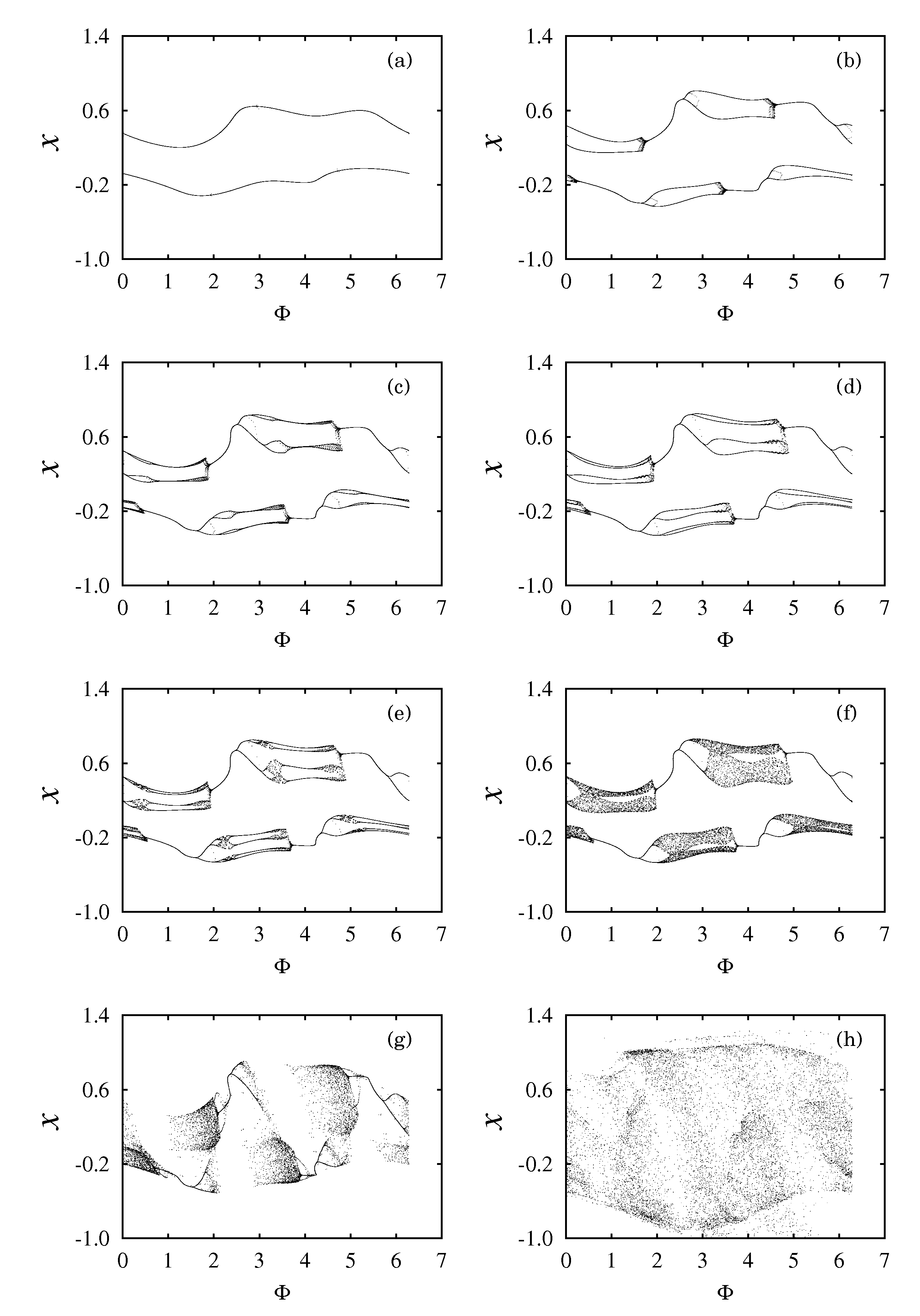
Figure 2: Projection of the numerically simulated Poincaré surface section plots of the attractors of Eqs. (2) in the ($\phi-x$) plane with $\phi$ modulo 2$\pi$ as a function of amplitude of the forcing $f_{1}$ including the transition from quasiperiodic attractors to SNA through bubble doubling route: (a) period$-$2 torus for $f_{1}$ $=$ $0.7296$, (b) bubbled strands of period$-$2 torus $f_{1}$ $=$ $0.7744$, (c & d) doubled bubble strands of the period$-$2 torus for $f_{1}$ $=$ $0.7770$ and $f_{1}$ $=$ $0.7803$, (e) bifurcated bubble, (f) SNA for $f_{1}$ $=$ $0.8200$, (g) merged two torus and (h) chaotic attractor for $f_{1}$ $=$ $0.9475$.

Further, increasing the $f_{1}$ value from $0.7744$ the bubbles get doubled as shown in Figs. 2(c & d). Beyond the value of $f_{1}$ $=$ $0.7803$, the bubbles get successive doubling Fig. 2(e) and cause the emergence of SNA. The SNA start to appears above the value of $f_{1}$ $=$ $0.8123$. It is to be noted that the remaining part of the strands of the torus remain unaffected. The Poincaré surface section plot of SNA for the value of $f_{1}$ $=$ $0.8200$ is shown in Fig. 2(f) and the corresponding power spectrum is shown in Fig. 3b(ii). Beyond the value of $f_{1}$$=$ $0.8200$, the bifurcated strands corresponding to period$-$2 torus merge into a single strand and then transit to chaotic attractor, which are shown in Fig. 2(g) and Fig. 2(h) respectively. The power spectrum of the chaotic attractors is shown in Fig. 3c(ii). These observations show clearly that the bubbles that appear in the strands of the torus undergo successive doubling and cause the emergence of strange nonchaotic dynamics. The mechanism for this route is that the quasiperiodic orbit becomes unstable as a function of control parameter and resulting the appearance of bubbles in certain parts of the main strands. Further increasing the control parameter these bubbles losses it’s stability and gets successive doubling and leads to birth of SNAs. These observations point out that this route is significantly different from other routes known in dynamical systems pras2 .

Figure 3: Projection of the numerically simulated attractors of Eqs. (2) with (i) Poincaré plot with $\phi$ modulo 2$\pi$ in the ($\phi-x$) plane and (ii) corresponding power spectrum for various value of $f_{1}$ indicating the transition from a quasiperiodic attractor to an SNA and chaos. (a) period$-$2 torus for $f_{1}$ $=$ $0.7296$, (b) SNA for $f_{1}$ $=$ $0.8200$ and (c) chaos for $f_{1}$ $=$ $0.9475$.

IV Lyapunov Exponent and its variance

To characterize the quasiperiodic, strange nonchaotic and chaotic dynamics, the largest Lyapunov exponent and its variance are calculated as functions of $f_{1}$ for the range of 0.8000 to 0.8500. The variance$(\sigma)$ of the largest asymptotic Lyapunov exponent $(\Lambda)$ from finite time Lyapunov exponents $(\bar{\lambda})$ of length M, and its variance defined as

$$\bar{\lambda} = \frac{1}{M}\sum_{i=1}^{M}\lambda_{i},$$ (3a)

$$\sigma = \frac{1}{K}\sum_{i=1}^{K}(\Lambda-\bar{\lambda_{i}})^{2}.$$ (3b)

Figure 4: Transition from two torus to chaos through SNA. (a) the largest Lyapunov exponent $\Lambda$ and (b) variance $\sigma$ as a function of parameter $f_{1}$.

where $K$ is the total number of finite LE (${\bar{\lambda}}$) and $\lambda_{i}$ is the instantaneous Lyapunov exponent. The plot of the largest Lyapunov exponent and its variance are shown in Figs. 4(a & b). It clearly demarcate the range of the three dynamical behaviours such as quasiperiodic, SNA and chaos. Below the value of $f_{1}$ $=$ $0.8123$ the system exhibits quasiperiodic behavior. In the range $f_{1}$ $=$ $0.8123$ to $f_{1}$ $=$ $0.8292$ the largest Lyapunov exponent is negative and the corresponding variance is higher in this range, is indicate the existence of SNA. The strange nonchaotic dynamics becomes chaotic dynamics beyond the value of $f_{1}$=0.8292 (after the largest Lyapunov exponent crosses zero axis).

V Singular Continuous spectrum analysis

The singular continuous spectrum analysis, which is used to quantitatively confirm the strange nonchaotic nature of the dynamics, was first proposed in the investigation of model of quasiperiodic lattices and quasiperiodically forced quantum systems aubr . In general, power spectra of dissipative dynamical system can be either discrete, or continuous, or a combination of both. Discrete spectrum are usually generated by regular motions such as periodic or quasiperiodic motions, where as continuous spectra correspond to irregular motions such as chaotic or random motion. A singular continuous spectrum is a mixture of both discrete and continuous spectra yalc . Using this property, we can identify whether the bubble doubling indeed leads to strange nonchaotic dynamics or not. To confirm this we compute the partial Fourier sum piko1 ; yalc1 as

$$X(\alpha,N)=\sum_{k=1}^{N}(x)_{k}\exp(2\pi ik\alpha)$$ (4)

where $\alpha$ is proportional to the irrational driving frequency $\Omega_{1}$ and $\{x_{k}\}$ is the time series of the variable $x$ of length N for the value of $f_{1}$ $=$ $0.8200$. When N is regarded as time, $|X(\alpha,N)|^{2}$ grows with time N as piko2

$$|X(\alpha,N)|^{2} \sim N^{\mu}$$ (5)

where $\mu$ is the scaling exponent. The time evolution of $X(\alpha,N)$ can be represented by an orbit or a walker in the complex plane $(Re[X(\alpha,N)],Im[X(\alpha,N)])$ and for a singular continuous spectrum (when the dynamics is strange) it implies that the walk on the plane $(Re[X(\alpha,N)],Im[X(\alpha,N)])$ will be a fractal piko1 .

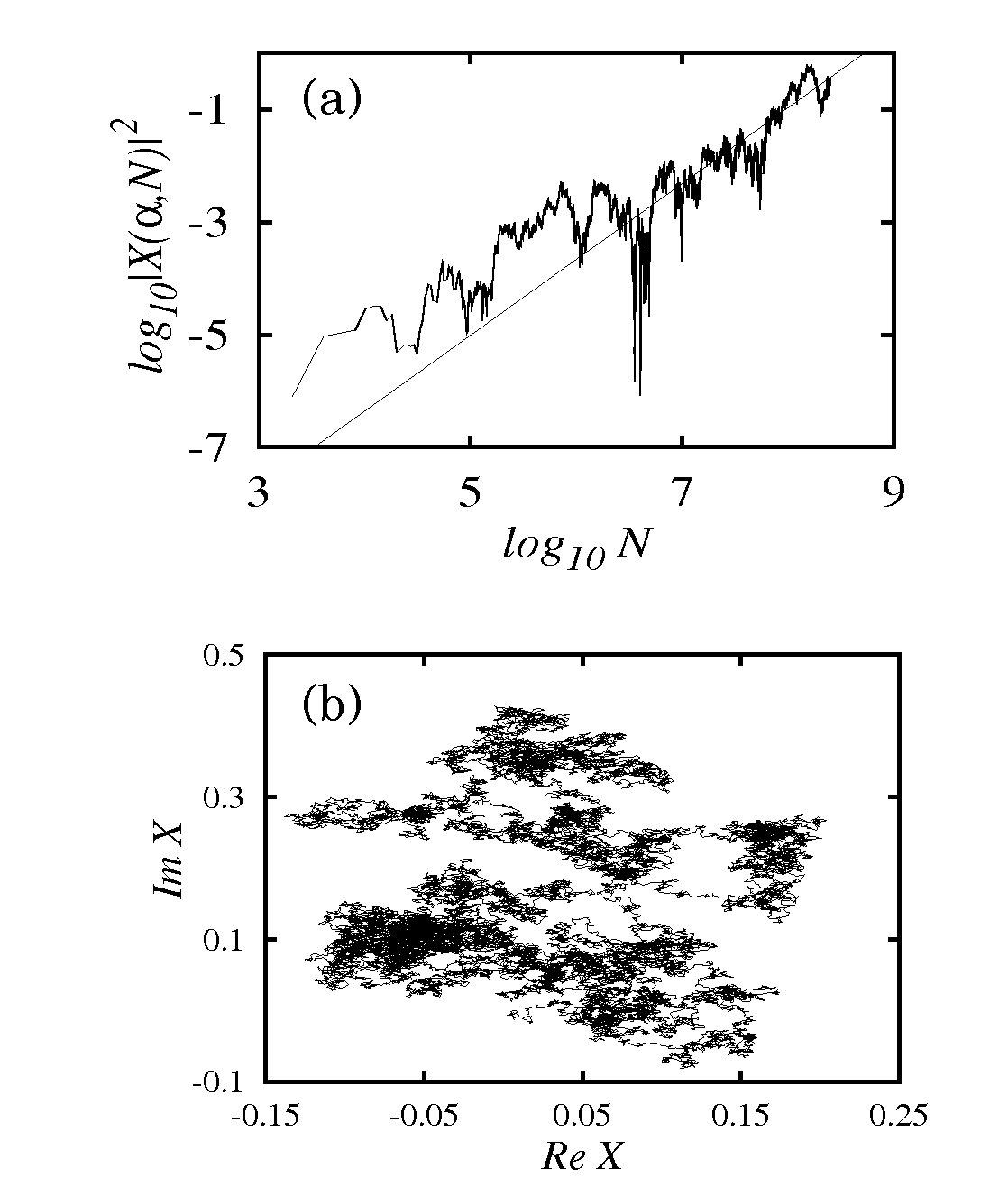
Figure 5: Singular continuous spectrum analysis of the $\{x_{k}\}$ time series at $f_{1}$ $=$ $0.8200$. (a) plot of $N$ $vs$ $|X(\alpha,N)|^{2}$ showing the power-law scaling; the slop is $\approx$ 1.345 and (b) the fractal path in the complex plane $(Re[X(\alpha,N)],Im[X(\alpha,N)])$

Fig. 5(a) shows, the plot of $N$ $vs$ $|X(\alpha,N)|^{2}$ for $\alpha$ $=$ $\Omega_{1}$/4, which has the scaling exponent $\mu$ $\approx$ 1.345 and the walk in Fig. 5(b) appears to be fractal. These results, $1<\mu<2$ and fractal walk, strongly suggest that the dynamics is indeed strange and nonchaotic.

VI separation of near by points

SNAs exhibit complicated geometrical structure like chaotic attractors. One way to distinguish SNAs from chaotic attractors is to look for the sensitive dependence on initial conditions venk1 . In order to verify this sensitive dependence, we analyse the separation $\Delta$ between two orbits starting from two near by initial conditions. For this two near by points on the attractor ($x_{i},y_{i},z_{i}$) and ($x_{j},y_{j},z_{j}$) are chosen and their separation

$$\small\Delta=\sqrt{(x_{i}-x_{j})^{2}+(y_{i}-y_{j})^{2}+(z_{i}-z_{j})^{2}}$$ (6)

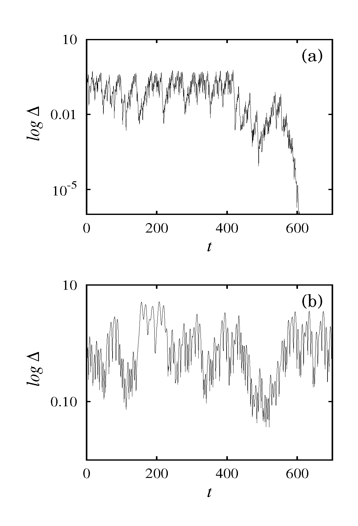
Figure 6: Separation of two nearby points vs time (t). (a) strange nonchaotic attractor for the value of $f_{1}$ $=$ $0.8200$ and (b) chaotic attractor for the value of $f_{1}$ $=$ $0.9475$.

is monitored at each forward step. For regular behaviour $\Delta$ will decay to zero as t$\rightarrow\infty$, but for chaotic behaviour, $\Delta$ becomes irregular. In Figs. (6) a plots of t versus $\Delta$ is shown. In Fig. 6(a) shows $\Delta$ for the value of $f_{1}$ $=$ $0.8200$ diminishes to zero in short interval of t and Fig. 6(b) shows $\Delta$ for $f_{1}$ $=$ $0.9475$ sustains the irregular variation for long time (t$\rightarrow\infty$). Hence the former case clearly supports the loss of sensitive dependence on initial condition, which corresponds to the strange nonchaotic attractor, while the later one corresponds to a chaotic attractor.

VII Distribution of finite time Lyapunov exponent

We have discussed about the bubble doubling dynamics qualitatively in section III, by using Poincaré surface of section plots in the $(\phi-x)$ plane, also quantitatively by using maximal Lyapunov exponent and sigular continuous spectrum analysis in section IV. In addition to the above it is also possible to distinguish torus and SNA using distribution of finite time Lyapunov exponent mani .

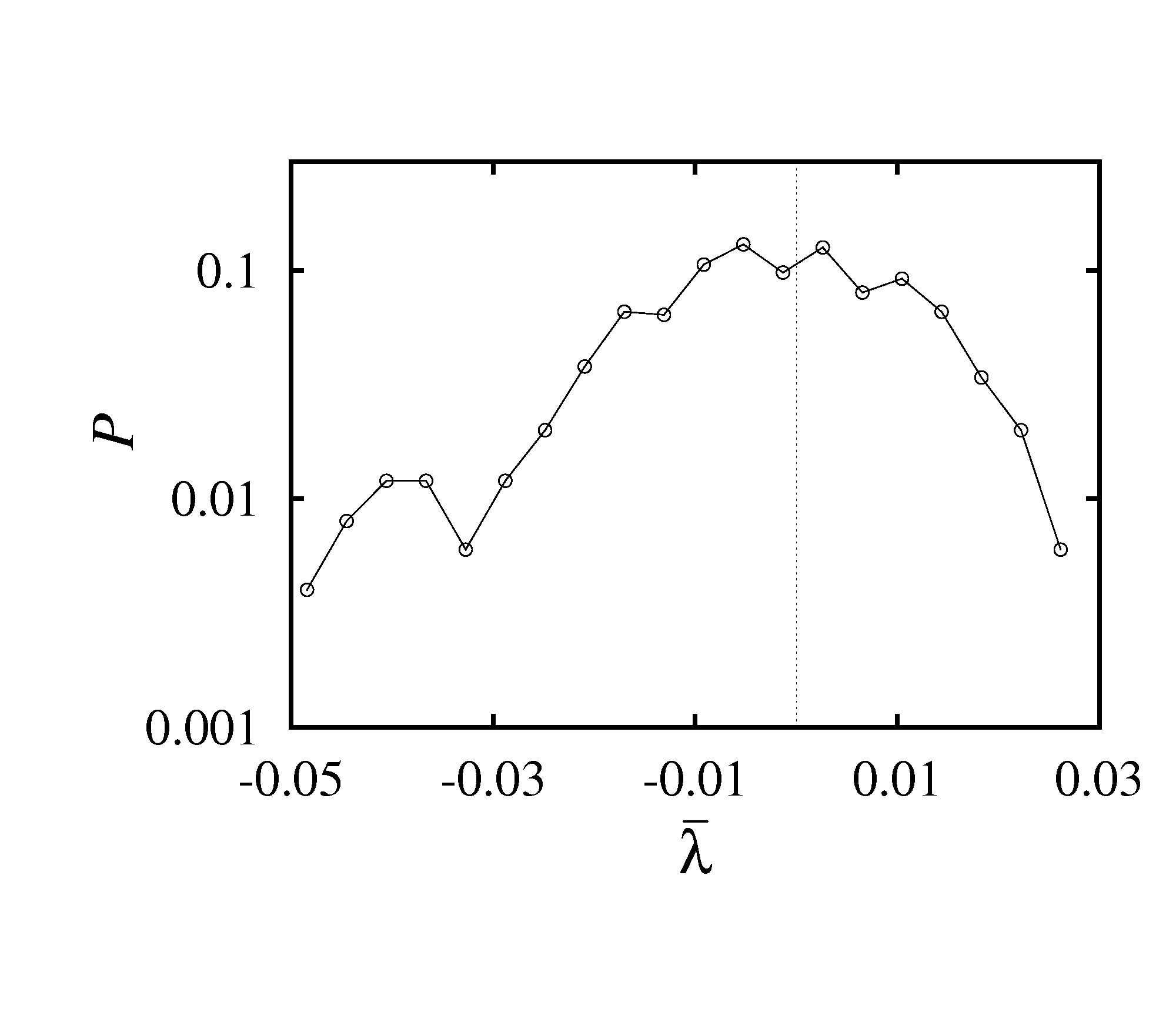
Figure 7: Distribution of finite time Lyapunov exponent is taken for $M=2000$ for the value of $f_{1}$ $=$ $0.8200$

It has been shown pras that a trajectory on a SNA actually possesses positive Lyapunov exponent in finite time intervals, although the asymptotic exponent is negative. As a consequence, it is possible to observe different characteristic of the SNA created through different mechanisms sent by studying the differences in the probability ($P$) of distribution of finite time Lyapunov exponent $P(M,\bar{\lambda})$ for positive and negative values. We have calculated the distribution of finite time Lyapunov exponent $P(2000,\bar{\lambda})$ for the attractor shown in Fig. 3b(i) and have plotted the same in Fig. (7). Here we find that the distribution exhibits an elongated tail for the negative values, thereby confirming the existence of bubble doubling transition to SNA. This may be explained as due to the fact that in the bubble doubling transition, the unaffected regions of the strands of the period$-$2 torus remain so even after the birth of SNA.

VIII Summary and conclusion

In this paper, we have reported a novel machanism for the birth of strange nonchaotic attractor in quasiperiodically forced Chua’s circuit. We term this route as bubble doubling route to SNA. At first, we have presented the appearence of bubble through Poincaré surface of cross section and the bifurcation of the bubble by varing the control parameter $f_{1}$ in the suitable range. Further, we used power spectrum to qualitatively distinguish quasiperiodicity, SNA and choatic attractor. Followed by this, we have computed Lyapunov exponent and its variance as a function of control parameter $f_{1}$ and these clearly distinguish the dynamical region of quasiperiodicity, SNA and chaos. To confirm the presence of SNA we have computed singular continuous spectrum, which clearly shows the fractal dimension of the SNA and its fractal path in the complex plane. The separation of near by point test and distribution of the finite time Lyapunov exponent also explains the presence of SNAs. It is to be noted that the formation of SNA through this bubble doubling mechanism is significantly different from the well known mechanisms in the literature (Table - I).

References

- (1) C. Grebogi, E. Ott, S. Pelikan and J. A. Yorke, Physica D 13, 261 (1984).
- (2) F. J. Romeiras and E. Ott, Phys. Rev. A 35, 4404 (1987); F. J. Romeiras, A. Bondeson, E. Ott, T. M. Andonsen, Jr., and C. Grebogi, Physica D 26, 277 (1987); Y. C. Lai, Phys. Rev. E 53, 57 (1996); T. Nishikawa, and K. Kaneko, ibid. 54, 6114 (1996).
- (3) A. Bondeson, E. Ott and T. M. Antonsen, Jr., Phys. Rev. Lett. 55, 2103 (1985).
- (4) M. Ding, C. Grebogi and E. Ott, Phys. Rev. A 39, 2593 (1989); M. Ding and J. A. Scott Relso, Int. J. Bifurcation Chaos Appl. Sci. Eng. 4, 533 (1994).
- (5) A. Venkatesan, M. Lakshmanan, A. Prasad and R. Ramaswamy, Phys. Rev. E 61, 3641 (2000).
- (6) J. F. Heagy and W. L. Ditto, J. Nonlinear Sci. 1, 423 (1991); J. I. Staglino, J. M. Wersinger and E. E. Slaminka, Physica D 92, 164 (1996).
- (7) T. Yalçinkaya and Y. C. Lai, Phys. Rev. Lett. 77, 5039 (1996).
- (8) T. Kapitaniak and J. Wojewoda, Attractors of Quasiperiodically Forced Systems (World Scientific, Singapore, 1993).
- (9) U. Feudel, S. Kuznetsov and A. Pikovsky, Strange Nonchaotic Attractors: Dynamics between Order and Chaos in Quasiperiodically Forced Systems (World Scientific, Singapore, 2006).
- (10) A. Venkatesan and M. Lakshmanan, Phys. Rev. E 55, 5134 (1997); A. Venkatesan and M. Lakshmanan, Phys. Rev. E 58, 3008 (1998).
- (11) T. Yang and K. Bilimgut, Phys. Lett. A 236, 494 (1997).
- (12) Z. Zhua and Z. Liu, Int. J. Bifurcation and Chaos, 7, 227 (1997).
- (13) A. Venkatesan, K. Murali and M. Lakshmanan, Phys. Lett. A 259, 246 (1999).
- (14) A. Prasad, V. Mehra and R. Ramaswamy, Phys. Rev. Lett. 79, 4127 (1997); A. Prasad, V. Mehra and R. Ramaswamy, Phys. Rev. E 57, 1576 (1998).
- (15) A. S. Pikovsky and U. Feudel, Chaos 5, 253 (1995); U. Feudel, J. Kurths, and A. S. Pikovsky, Physica D 88, 176 (1995). Í“
- (16) A. S. Pikovsky and U. Feudel, J. Phys. A 27, 5209 (1994).
- (17) T. Yalçinkaya and Y. C. Lai, Phys. Rev. E 56, 1623 (1997) Í“
- (18) S. P. Kuznetsov, A. S. Pikovsky and U. Feudel, Phys. Rev. E 51, R1629 (1995); A. Witt, U. Feudel and A. S. Pikovsky, Physica D 109, 180 (1997). Í“
- (19) V. S. Anishchenko, T. E. Vadivasova and O. Sosnovtseva, Phys. Rev. E 53, 4451 (1996); O. Sosnovtseva, U. Feudel, J. Kurths and A. S. Pikovsky, Phys. Lett. A 218, 225 (1996); S. Kuznetsov, U. Feudel and A. Pikovsky, Phys. Rev. E 57, 1585 (1998).
- (20) T. Nishikawa and K. Kaneko, Phys. Rev. E 54, 6114 (1996).
- (21) A. Venkatesan and M. Lakshmanan, Phys. Rev. E 63, 026219 (2001). Í“
- (22) B. R. Hunt and E. Ott, Phys. Rev. Lett. 87, 254101 (2001); J.W. Kim, S. Y. Kim, B. Hunt and E. Ott, Phys. Rev. E 67, 036211 (2003).
- (23) S. Y. Kim, W. Lim and E. Ott, Phys. Rev. E 67, 056203 (2003). Í“
- (24) W. Lim and S. Y. Kim, J. Korean Phys. Soc. 3, 514 (2004).
- (25) J. F. Heagy and S. M. Hammel, Physica D 70, 140 (1994).
- (26) W. L. Ditto, M. L. Spano, H. T. Savage, S. N. Rauseo, J. Heagy and E. Ott, Phys. Rev. Lett. 65, 533 (1990).
- (27) T. Zhou, F. Moss and A. Bulsara, Phys. Rev. A 45, 5394 (1992). Í“
- (28) W. X. Ding, H. Deutsch, A. Dinklage and C. Wilke, Phys. Rev. E 55, 3769 (1997). Í“
- (29) J. A. Ketoja and I. Satija, Physica D 109, 70 (1997). Í“Í“
- (30) A. Prasad, R. Ramaswamy, I. I. Satija and N. Shah, Phys. Rev. Lett. 83, 4530 (1999). Í“Í“
- (31) C. S. Zhou and T. L. Chen, Europhys. Lett. 38, 261 (1997). Í“Í“
- (32) R. Ramaswamy, Phys. Rev. E 56, 7294 (1997). Í“Í“
- (33) R. Chacon and A. M. Gracia-Hoz, Europhys. Lett. 57, 7 (2002).
- (34) A. Prasad, S. S. Negi and R. Ramaswamy, Int. J. Bifurcation Chaos Appl. Sci. Eng. 11, 291 (2001).
- (35) D. V. Senthilkumar, K. Srinivasan, K. Thamilmaran and M. Lakshmanan, Phys. Rev. E 78, 066211 (2008).
- (36) M. Agrawal, A. Prasad and R. Ramaswamy, Phys. Rev. E 81, 026202 (2010).
- (37) S. Aubry, C. Godreche, and J. M. Luck, Europhys. Lett. 4, 639 (1987); J. Stat. Phys. 51, 1033 (1988); C. Godreche,J. M. Luck and F. Vallet, J. Phys. A 20, 4483 (1987); J. M. Luck, H. Orland and U. Smilansky, J. Stat. Phys. 53, 551 (1988).
- (38) A. S. Pikovsky, M. A. Zaks, U. Feudel and J. Kurths, Phys. Rev. E 52, 285 (1995).