Quantum dynamics of a binary mixture of BECs in a double well potential: an Holstein-Primakoff approach

Abstract

We study the quantum dynamics of a binary mixture of Bose-Einstein condensates (BEC) in a double-well potential starting from a two-mode Bose-Hubbard Hamiltonian. Focussing on the regime where the number of atoms is very large, a mapping onto a $SU(2)$ spin problem together with a Holstein-Primakoff transformation is performed. The quantum evolution of the number difference of bosons between the two wells is investigated for different initial conditions, which range from the case of a small imbalance between the two wells to a coherent spin state. The results show an instability towards a phase-separation above a critical positive value of the interspecies interaction while the system evolves towards a coherent tunneling regime for negative interspecies interactions. A comparison with a semiclassical approach is discussed together with some implications on the experimental realization of phase separation with cold atoms.

I Introduction

Bose-Einstein condensates of dilute, weakly interacting gases offer a unique possibility for exploring many-body dynamics, the role of quantum fluctuations and in general macroscopic quantum coherence phenomena leggett1 , thanks to a wide tunability of the interaction parameters. Indeed several experimental strategies can be devised in order to pursue this task, which range from the direct control via magnetic Feshbach resonance techniques control1 to the transverse confinement in a quasi one dimensional system control2 as a way to increase the inter-atomic interaction. Finally, the introduction of an optical lattice whose depth can be tuned allows one to decrease the kinetic term in the Hamiltonian. Within the tight binding approximation such systems are described by the Bose-Hubbard Hamiltonian, whose parameters are the hopping frequency $\overline{E}_{J}$ between nearest neighbor lattice sites, the onsite interaction strength $E_{c}$ and the total atoms number $N$. When the ratio $\frac{E_{c}N}{\overline{E}_{J}}$ exceeds unity, a quantum phase transition from a superfluid to a Mott insulator mott1 takes place and the system enters a quantum regime characterized by strong correlations. The simplest Hamiltonian of this kind that one can devise is the Bose-Hubbard dimer dimer1 , which describes the physics of two weakly coupled condensates. It can be mapped onto a $SU(2)$ spin problem and is deeply related to the physics of Josephson junctions gati1 ferrini1 leggett1 . Furthermore, if the mean field approximation is considered one obtains the Gross-Pitaevskii theory which gives rise to a variety of phenomena, ranging from Josephson oscillations jos1 to macroscopic quantum self-trapping (MQST) smerzi1 and ac and dc Josephson like effect smerzi2 , all experimentally observed in the last decade exp1 exp2 exp3 .

More recently, after the experimental realization of two-species BECs exp4 exp5 exp6 , the theoretical analysis on weakly coupled condensates has been successfully extended to a binary mixture of BECs in a double well potential mix0 mix1 mix2 mix3 mix4 mix4bis . The semiclassical regime in which the fluctuations around the mean values are small has been deeply investigated and found to be described by two coupled Gross-Pitaevskii equations. By means of a two-mode approximation such equations can be cast in the form of four coupled nonlinear ordinary differential equations for the population imbalance and the relative phase of each species. The solution results in a richer tunneling dynamics mix5 . In particular, two different MQST states with broken symmetry have been found mix3 , where the two species localize in the two different wells giving rise to a phase separation or coexist in the same well respectively. Indeed, upon a variation of some parameters or initial conditions, the phase-separated MQST states evolve towards a symmetry-restoring phase where the two components swap places between the two wells, so avoiding each other. Furthermore the coherent dynamics of a two species BEC in a double well has been analyzed as well focussing on the case where the two species are two hyperfine states of the same alkali metal mix6 .

In a recent paper noi1 we studied the quantum behaviour of a binary mixture of Bose-Einstein condensates (BEC) in a double-well potential starting from a two-mode Bose-Hubbard Hamiltonian. We analyzed in detail the small tunneling amplitude regime where number fluctuations are suppressed and a Mott-insulator behaviour is established. Within this regime we performed a perturbative calculation up to second order in the tunneling amplitude and found the stationary states. In order to carry out analytical calculations we focused on the symmetric case of equal nonlinear interaction and equal tunneling amplitude of the two species. Furthermore we restricted to the case in which the two species are equally populated and imposed the condition of equal population imbalance of the species $a$ and $b$ between the two wells. Then, the dynamics of the junction was investigated in correspondence of a completely localized initial state. In order to avoid the above restrictions on the parameters range, here we focus on the two-mode Bose-Hubbard Hamiltonian describing the two-species BEC ($a$ and $b$) in a double well when $N_{a},N_{b}\gg 1$, and perform a mapping onto a $SU(2)$ spin problem together with a Holstein-Primakoff transformationhp1 hp2 . As a result we obtain a Hamiltonian of two decoupled quantum harmonic oscillators, similar to that of Ref.hp3 , whose stationary states are readily found. The quantum evolution of the number difference of bosons between the two wells is investigated in detail in correspondence of a variety of initial conditions, which range from an initial state with small imbalance between the two species to a coherent spin state. The whole parameters space is explored by tuning the population, the tunneling amplitude and the nonlinear interaction for each species as well as the interspecies interaction in a wide range, from a symmetric to a strongly asymmetric case. Finally a detailed comparison with a semiclassical approach is given. Let us notice that Holstein-Primakoff transformation makes the system exactly solvable in the weakly interacting regime of interest in this work and that simplifies the study of the tunneling dynamics as well as the phase separation phenomenon. This is the main advantage of the approach chosen.

The paper is organized as follows. In Section 2 we introduce the model Hamiltonian we study within the two mode approximation. A Holstein-Primakoff transformation is performed and the semiclassical limit is taken followed by a decoupling of the bosonic degrees of freedom for each species. As a result the Hamiltonian can be rephrased in terms of two independent harmonic oscillators, whose stationary states are derived in Section 3. In Section 4 the quantum dynamics of the system is discussed in correspondence of two different initial conditions: small imbalance between the two wells and coherent states. A wide range of values of interspecies interaction is explored and the crossover to an unstable regime with phase separation is found. In Section 5 the classical equations of motion are derived and a comparison with the quantum counterpart is carried out. Finally some conclusions and perspectives of this work are briefly outlined.

II The model

A binary mixture of Bose-Einstein condensates mix1 mix3 loaded in a double-well potential is described by the Hamiltonian $H=H_{a}+H_{b}+H_{ab}$ where:

$$H_{i}=\int d\overrightarrow{r}\left(-\frac{\hbar^{2}}{2m_{i}}\psi_{i}^{+}\nabla^{2}\psi_{i}+\psi_{i}^{+}V_{i}\left(\overrightarrow{r}\right)\psi_{i}\right)+\frac{g_{ii}}{2}\int d\overrightarrow{r}\psi_{i}^{+}\psi_{i}^{+}\psi_{i}\psi_{i};\text{ \ \ \ }i=a,b$$ (1)

$$H_{ab}=g_{ab}\int d\overrightarrow{r}\psi_{a}^{+}\psi_{b}^{+}\psi_{a}\psi_{b}.$$ (2)

Here $g_{ii}=\frac{4\pi\hbar^{2}a_{ii}}{m_{i}}$ is the intraspecies coupling constants, being $m_{i}$ the atomic mass and $a_{ii}$ the $s$-wave scattering lengths; $g_{ab}=\frac{2\pi\hbar^{2}a_{ab}}{m_{ab}}$ is the interspecies coupling constant, where $m_{ab}=\frac{m_{a}m_{b}}{m_{a}+m_{b}}$ is the reduced mass; $V_{i}\left(\overrightarrow{r}\right)$ is the double well trapping potential and, in the following, we assume $V_{a}\left(\overrightarrow{r}\right)=V_{b}\left(\overrightarrow{r}\right)=V\left(\overrightarrow{r}\right)$; $\psi_{i}^{+}\left(\overrightarrow{r}\right),$ $\psi_{i}\left(\overrightarrow{r}\right)$, $i=a,b$ are the bosonic creation and annihilation operators for the two species, which satisfy the commutation rules:

$$\left[\psi_{i}\left(\overrightarrow{r}\right),\psi_{j}\left(\overrightarrow{r}^{\prime}\right)\right] = \left[\psi_{i}^{+}\left(\overrightarrow{r}\right),\psi_{j}^{+}\left(\overrightarrow{r}^{\prime}\right)\right]=0,$$ (3)

$$\left[\psi_{i}\left(\overrightarrow{r}\right),\psi_{j}^{+}\left(\overrightarrow{r}^{\prime}\right)\right] = \delta_{ij}\delta\left(\overrightarrow{r}-\overrightarrow{r}^{\prime}\right),\text{ \ \ \ \ }i,j=a,b,$$ (4)

and the normalization conditions:

$$\int d\overrightarrow{r}\left|\psi_{i}\left(\overrightarrow{r}\right)\right|^{2}=N_{i};\text{ \ \ \ }i=a,b,$$ (5)

$N_{i}$, $i=a,b$ being the number of atoms of species $a$ and $b$ respectively. The total number of atoms of the mixture is $N=N_{a}+N_{b}$.

A weak link between the two wells produces a small energy splitting between the mean-field ground state and the first excited state of the double well potential and that allows to reduce the dimension of the Hilbert space of the initial many-body problem. Indeed for low energy excitations and low temperatures it is possible to consider only such two states and neglect the contribution from the higher ones, the so called two-mode approximation milburn smerzi1 ananikian1 . In this approximation the Hamiltonian (1) can be written in terms of the the annihilation operators, $a_{L}=\frac{1}{\sqrt{2}}\left(a_{g}+a_{e}\right)$, $a_{R}=\frac{1}{\sqrt{2}}\left(a_{g}-a_{e}\right)$ and $b_{L}=\frac{1}{\sqrt{2}}\left(b_{g}+b_{e}\right)$, $b_{R}=\frac{1}{\sqrt{2}}\left(b_{g}-b_{e}\right)$ and the corresponding creation operators, where $a_{g},a_{e}$ and $b_{g},b_{e}$ are the annihilation operators of a particle in the ground and in the first excited state.

When introducing the angular momentum operators:

$$\begin{array}[]{ccc}J_{x}^{a}=\frac{1}{2}\left(a_{R}^{+}a_{L}+a_{L}^{+}a_{R}\right),&J_{y}^{a}=\frac{i}{2}\left(a_{R}^{+}a_{L}-a_{L}^{+}a_{R}\right),&J_{z}^{a}=\frac{1}{2}\left(a_{R}^{+}a_{R}-a_{L}^{+}a_{L}\right),\\ J_{x}^{b}=\frac{1}{2}\left(b_{R}^{+}b_{L}+b_{L}^{+}b_{R}\right),&J_{y}^{b}=\frac{i}{2}\left(b_{R}^{+}b_{L}-b_{L}^{+}b_{R}\right)&J_{z}^{b}=\frac{1}{2}\left(b_{R}^{+}b_{R}-b_{L}^{+}b_{L}\right),\end{array}$$ (6)

where the operators $J_{i}^{a}$, $J_{i}^{b}$, $i=x,y,z$, obey to the usual angular momentum algebra together with the relation:

$$\begin{array}[]{cc}\left(J^{a}\right)^{2}=\frac{N_{a}}{2}\left(\frac{N_{a}}{2}+1\right),&\left(J^{b}\right)^{2}=\frac{N_{b}}{2}\left(\frac{N_{b}}{2}+1\right),\end{array}$$ (7)

the Hamiltonian of the double species Bose-Josephson junction can be written in the form:

$$H = \frac{1}{2}\Lambda_{a}\left(J_{z}^{a}\right)^{2}-K_{a}J_{x}^{a}+C_{a}\left(J_{x}^{a}\right)^{2}+\frac{1}{2}\Lambda_{b}\left(J_{z}^{b}\right)^{2}-K_{b}J_{x}^{b}+C_{b}\left(J_{x}^{b}\right)^{2}+$$ (8)

$$+\Lambda_{ab}J_{z}^{a}J_{z}^{b}-D_{ab}J_{x}^{a}J_{x}^{b}.$$

where $K_{a,b}$ are the tunneling amplitudes between the two wells, $\Lambda_{a,b},\Lambda_{ab}$ are the intra- and interspecies interactions respectively, while the terms $C_{a}$ and $D_{a,b}$ describe two-particle processes noi1 . The form (8) was previously discussed in the classical limit in mix3 , where it was shown to be lead to equations of motion equivalent to the Gross-Pitaevskii equations. For $\Lambda_{ab}=D_{ab}=0$ in Eq. (8), the Hamiltonian reduces to a sum of two Lipkin-Meshkov-Glick (LMG) model lipkin1 ; lipkin2 Hamiltonian, one for each species. For $\Lambda_{ab}\neq 0$ or $D_{ab}\neq 0$, the two LMG models are coupled. Within the experimental parameters range it is possible to show that $C_{i}\ll\Lambda_{i},K_{i}$, $i=a,b$, and $D_{ab}\ll\Lambda_{ab}$ noi1 gati1 mix3 , then in the following we put $C_{a}=C_{b}=0$ and $D_{ab}=0$, which corresponds to neglecting the spatial overlap integrals between the localized modes in the two wells. In this way the binary mixture of BECs within two-mode approximation maps to a two Ising spins model in a transverse magnetic field, whose Hamiltonian is:

$$H=\frac{1}{2}\Lambda_{a}\left(J_{z}^{a}\right)^{2}-K_{a}J_{x}^{a}+\frac{1}{2}\Lambda_{b}\left(J_{z}^{b}\right)^{2}-K_{b}J_{x}^{b}+\Lambda_{ab}J_{z}^{a}J_{z}^{b}.$$ (9)

Let us briefly discuss the symmetries of the Hamiltonian (9). First, when $\Lambda_{ab}=0$, the Hamiltonian decouples into $H=H_{a}+H_{b}$, and $e^{i\pi J_{x}^{\nu}}H_{\nu^{\prime}}e^{-i\pi J_{x}^{\nu}}=H_{\nu^{\prime}}$ for $\nu,\nu^{\prime}\in\{a,b\}$. Therefore, the eigenstates of $H$ can be sought in the form of eigenstates of $e^{i\pi J_{x}^{a}}$ and $e^{i\pi J_{x}^{b}}$. Since $e^{2i\pi J_{x}^{\nu}}=e^{i\pi N_{\nu}}$, these eigenvalues are $\pm 1$ when $N_{\nu}$ is even, and $\pm i$ when $N_{\nu}$ is odd. So the Hilbert space breaks down into four sectors indexed by the eigenvalues of $e^{i\pi J_{x}^{a}}$ and $e^{i\pi J_{x}^{b}}$. Then, turning on $\Lambda_{ab}\neq 0$, the only remaining symmetry is $e^{i\pi(J_{x}^{a}+J_{x}^{b})}H_{\nu^{\prime}}e^{-i\pi(J_{x}^{a}+J_{x}^{b})}$, so that only two independent sectors remain. These sectors are formed by the combination in pairs of the four sectors obtained for $\Lambda_{ab}=0$.

Let us now make the rotation:

$$\begin{array}[]{cc}\begin{array}[]{c}J_{z}^{i}\rightarrow-J_{x}^{i}\\ J_{x}^{i}\rightarrow J_{z}^{i}\end{array},&i=a,b.\end{array}$$ (10)

To proceed we perform the Holstein-Primakoff transformation hp1 ; hp2 ; hp3 in order to map the angular momentum operators into bosonic ones and focus on the regime with large number of atoms $N_{a},N_{b}\gg 1$ and weak scattering strengths $K_{a(b)}\gg\Lambda_{a},\Lambda_{b},\Lambda_{ab}$:

$$\begin{array}[]{c}J_{z}^{a}=J^{a}-a^{\dagger}a\\ J_{+}^{a}=\sqrt{2J^{a}-a^{\dagger}a}a\\ J_{-}^{a}=a^{\dagger}\sqrt{2J^{a}-a^{\dagger}a}\end{array},\begin{array}[]{c}J_{z}^{b}=J^{b}-b^{\dagger}b\\ J_{+}^{b}=\sqrt{2J^{b}-b^{\dagger}b}b\\ J_{-}^{b}=b^{\dagger}\sqrt{2J^{b}-b^{\dagger}b}\end{array},$$ (11)

where $J_{\pm}^{i}=J_{x}^{i}\pm iJ_{y}^{i},\;i=a,b$, $J^{i}=N_{i}/2\;i=a,b$, thus leading to the Hamiltonian:

$$H = \frac{\Lambda_{a}}{8}\left[2J^{a}(J^{a}+1)-2(J^{a}-a^{\dagger}a)^{2}+\sqrt{(2J^{a}-a^{\dagger}a)(2J^{a}-1-a^{\dagger}a)}a^{2}+(a^{\dagger})^{2}\sqrt{(2J^{a}-a^{\dagger}a)(2J^{a}-1-a^{\dagger}a)}\right]$$ (12)

$$+\frac{\Lambda_{b}}{8}\left[2J^{b}(J^{b}+1)-2(J^{b}-b^{\dagger}b)^{2}+\sqrt{(2J^{b}-b^{\dagger}b)(2J^{b}-1-b^{\dagger}b)}b^{2}+(b^{\dagger})^{2}\sqrt{(2J^{a}-b^{\dagger}b)(2J^{a}-1-b^{\dagger}b)}\right]$$

$$+\frac{\Lambda_{ab}}{4}\left[\sqrt{(2J^{a}-a^{\dagger}a)(2J^{b}-b^{\dagger}b)}ab+b^{\dagger}a^{\dagger}\sqrt{(2J^{a}-a^{\dagger}a)(2J^{b}-b^{\dagger}b)}\right.$$

$$\left.+\sqrt{2J^{b}-b^{\dagger}b}a^{\dagger}b\sqrt{2J^{a}-a^{\dagger}a}+\sqrt{2J^{a}-a^{\dagger}a}b^{\dagger}a\sqrt{2J^{a}-a^{\dagger}a}\right]$$

$$+K_{a}(a^{\dagger}a-J^{a})+K_{b}(b^{\dagger}b-J^{b}).$$

Here $a$ and $b$ are boson annihilation operators for each species. In this representation, the operators $e^{i\pi J_{z}^{\nu}}$ are equal to $e^{i\pi(J^{\nu}-\nu^{\dagger}\nu)}$ and their action is simply $\nu\to-\nu$. For $\Lambda_{ab}=0$, the Hilbert space of (12) thus breaks into four different sectors, according to the parity of $a^{\dagger}a$ and $b^{\dagger}b$, while for $\Lambda_{ab}\neq 0$, it breaks into two different sectors depending on the parity of $a^{\dagger}a+b^{\dagger}b$. The physical Hilbert space is restricted to $0\leq a^{\dagger}a\leq N_{a}$ and $0\leq b^{\dagger}b\leq N_{b}$.

Since we are considering a large number of atoms, we have $J^{a},J^{b}\gg 1$, while the condition $K_{a(b)}\gg\Lambda_{a},\Lambda_{b},\Lambda_{ab}$ implies $\langle a^{+}a\rangle\ll 2J^{a}$ and $\langle b^{+}b\rangle\ll 2J^{b}$. Under these assumptions one can use the linearized Holstein-Primakoff transformation hp1 (i.e. $J_{z}^{s}=J^{s}-s^{\dagger}s,J_{+}^{s}=\sqrt{2J^{s}}s,J_{-}^{s}=s^{\dagger}\sqrt{2J^{s}}$ with $s=a,b$) and derive the effective Hamiltonian:

$$H = \Lambda_{a}J^{a}\left(\frac{a+a^{+}}{2}\right)\left(\frac{a+a^{+}}{2}\right)+\Lambda_{b}J^{b}\left(\frac{b+b^{+}}{2}\right)\left(\frac{b+b^{+}}{2}\right)+$$ (13)

$$2\Lambda_{ab}\sqrt{J^{a}J^{b}}\left(\frac{a+a^{+}}{2}\right)\left(\frac{b+b^{+}}{2}\right)-K_{a}J^{a}-K_{b}J^{b}+K_{a}a^{+}a+K_{b}b^{+}b.$$

In order to decouple the degrees of freedom of each bosonic species let us introduce the following harmonic oscillator coordinates and momenta, $q_{i}$, $p_{i}$, $i=a,b$:

$$\begin{array}[]{cc}q_{a}=\frac{1}{\sqrt{2}}\left(a+a^{+}\right),&q_{b}=\frac{1}{\sqrt{2}}\left(b+b^{+}\right)\\ p_{a}=\frac{-i}{\sqrt{2}}\left(a-a^{+}\right)&p_{b}=\frac{-i}{\sqrt{2}}\left(b-b^{+}\right)\end{array},$$ (14)

which satisfy the usual commutation rules $\left[q_{i},p_{j}\right]=i\delta_{ij}$, $i,j=a,b$. Then, by defining:

$$\begin{array}[]{cc}Q_{a}=\frac{q_{a}}{\sqrt{K_{a}}},&Q_{b}=\frac{q_{b}}{\sqrt{K_{b}}},\\ P_{a}=\sqrt{K_{a}}p_{a},&P_{b}=\sqrt{K_{b}}p_{b},\end{array}$$ (15)

(where $\left[Q_{i},P_{j}\right]=i\delta_{ij}$, $i,j=a,b$) and, by dropping constant terms, Eq. (13) can be written in a matrix form as hp3 :

$$\widehat{H}_{2BJJ}\simeq\frac{1}{2}\left[\hat{Q}^{T}\widehat{\omega}^{2}\hat{Q}+\hat{P}^{T}\hat{P}\right],$$ (16)

where

$$\widehat{\omega}^{2}=\left(\begin{array}[]{cc}\omega_{a}^{2}&\omega_{ab}\\ \omega_{ab}&\omega_{b}^{2}\end{array}\right)$$ (17)

and $\hat{Q}^{T}=(Q_{a},Q_{b})$, $\hat{P}^{T}=(P_{a},P_{b})$ (the symbol $\cdot^{T}$ stands for the transpose); $\omega_{i}^{2}=\Lambda_{i}J^{i}K_{i}+K_{i}^{2}$, and $\omega_{ab}=\Lambda_{ab}\sqrt{J^{a}J^{b}K_{a}K_{b}}$.

A straightforward diagonalization gives the Hamiltonian:

$$H_{2BJJ}\simeq\frac{1}{2}\left[\omega_{1}^{2}Q_{1}^{2}+P_{1}^{2}+\omega_{2}^{2}Q_{2}^{2}+P_{2}^{2}\right],$$ (18)

where, defining $\Delta_{ab}=\sqrt{\left(\omega_{a}^{2}-\omega_{b}^{2}\right)^{2}+4\omega_{ab}^{2}}$,

$$\begin{array}[]{cc}\omega_{1}^{2}=\frac{\omega_{a}^{2}+\omega_{b}^{2}-\Delta_{ab}}{2},&\omega_{2}^{2}=\frac{\omega_{a}^{2}+\omega_{b}^{2}+\Delta_{ab}}{2}\end{array},$$ (19)

$$\begin{array}[]{cc}Q_{1}=\frac{\left\{2\omega_{ab}Q_{b}-\left[\left(\omega_{b}^{2}-\omega_{a}^{2}\right)+\Delta_{ab}\right]Q_{a}\right\}}{\sqrt{4\omega_{ab}^{2}+\left[\left(\omega_{b}^{2}-\omega_{a}^{2}\right)+\Delta_{ab}\right]^{2}}},&Q_{2}=\frac{\left\{2\omega_{ab}Q_{b}-\left[\left(\omega_{b}^{2}-\omega_{a}^{2}\right)-\Delta_{ab}\right]Q_{a}\right\}}{\sqrt{4\omega_{ab}^{2}+\left[\left(\omega_{b}^{2}-\omega_{a}^{2}\right)-\Delta_{ab}\right]^{2}}},\end{array}$$ (20)

$$\begin{array}[]{cc}P_{1}=\frac{\left\{2\omega_{ab}P_{b}-\left[\left(\omega_{b}^{2}-\omega_{a}^{2}\right)+\Delta_{ab}\right]P_{a}\right\}}{\sqrt{4\omega_{ab}^{2}+\left[\left(\omega_{b}^{2}-\omega_{a}^{2}\right)+\Delta_{ab}\right]^{2}}},&P_{2}=\frac{\left\{2\omega_{ab}P_{b}-\left[\left(\omega_{b}^{2}-\omega_{a}^{2}\right)-\Delta_{ab}\right]P_{a}\right\}}{\sqrt{4\omega_{ab}^{2}+\left[\left(\omega_{b}^{2}-\omega_{a}^{2}\right)-\Delta_{ab}\right]^{2}}}.\end{array}$$ (21)

The operators $Q_{1},P_{1}$ and $Q_{2},P_{2}$ can be viewed as position and momentum operators of two distinct fictitious particles, associated with the modes $1$ and $2$, i.e. the Hamiltonian (18) is that of two harmonic oscillators.

The eigenvalues $\omega_{1,2}$ up to order $K_{i}^{2}$ obtained within the Holstein-Primakoff approach coincide with the zero mode frequencies of small amplitude oscillations obtained by the semiclassical approach based on the Gross-Pitaevskii equations for the two condensate wave functions in Ref. mix1 (see Eq. (26)) and in Ref. mix3 (see Equation at the beginning of Section IV) for the case of equally populated species. When $\omega_{1}^{2}$ vanishes, a phase separation takes place, resulting in a MQST state.

Indeed, from Eqs. (19) the stability condition is:

$$\left|\Lambda_{ab}\right|<\sqrt{\left(\Lambda_{a}+\frac{K_{a}}{J^{a}}\right)\left(\Lambda_{b}+\frac{K_{b}}{J^{b}}\right)}=\Lambda^{c}_{ab},$$ (22)

where $\Lambda^{c}_{ab}$ is the critical value of the interspecies interaction which sets the onset of phase separation regime. Such a condition agrees the one given in Ref. mix3 (see Equation (10) in Section IV) and reduces to:

$$\left|\Lambda_{ab}\right|<\sqrt{\Lambda_{a}\Lambda_{b}},$$ (23)

when the limit $J^{a},J^{b}\rightarrow\infty$ is taken.

In the symmetric case $\Lambda_{a}=\Lambda_{b}=\Lambda$, $K_{a}=K_{b}=K$, $N_{a}=N_{b}=\frac{N}{2}$ we get $\omega_{a}^{2}=\omega_{b}^{2}=\omega^{2}$ where $\omega^{2}=\Lambda\frac{N}{2}K+K^{2}$, and $\omega_{ab}=\Lambda_{ab}\frac{N}{2}K$. As a consequence $\Delta_{ab}=2\omega_{ab}$ and the eigenvalues (19) simplify as:

$$\begin{array}[]{cc}\omega_{1}^{2}=\omega^{2}-\omega_{ab},&\omega_{2}^{2}=\omega^{2}+\omega_{ab}\end{array},$$ (24)

which result in the stability condition:

$$\left|\Lambda_{ab}\right|<\Lambda+2\frac{K}{N}=\Lambda^{c}_{ab}.$$ (25)

In the next Sections we will derive the analytical expressions for the stationary states and discuss the corresponding quantum dynamics of the system.

III Stationary states

Since the Hamiltonian (18) is that of two independent particles $H=H_{1}+H_{2}$, the corresponding Hilbert space is simply given by the tensor product $\mathcal{E}_{a}\otimes\mathcal{E}_{b}\equiv\mathcal{E}_{1}\otimes\mathcal{E}_{2}$ and we can find a basis of eigenvectors for $H_{2BJJ}$ in the following form: $\left|\varphi\right\rangle=\left|\varphi^{1}\right\rangle\left|\varphi^{2}\right\rangle$, where $\left|\varphi^{1}\right\rangle$ and $\left|\varphi^{2}\right\rangle$ are eigenvectors of $H_{1}$ and $H_{2}$ within $\mathcal{E}_{1}$ and $\mathcal{E}_{2}$. Since $H_{1}$ and $H_{2}$ are simply harmonic oscillator Hamiltonians, we could define two pairs of creation and annihilation operators, one for each mode, as follows:

$$\begin{array}[]{cc}a_{i}^{+}=\frac{1}{\sqrt{2}}\left[\sqrt{\frac{\omega_{i}}{\hbar}}Q_{i}-i\frac{P_{i}}{\sqrt{\omega_{i}\hbar}}\right],\end{array}$$ (26)

$$\begin{array}[]{cc}a_{i}=\frac{1}{\sqrt{2}}\left[\sqrt{\frac{\omega_{i}}{\hbar}}Q_{i}+i\frac{P_{i}}{\sqrt{\omega_{i}\hbar}}\right],\end{array}$$ (27)

being $i=1,2$. Now, if we define the ground states of $H_{1}$ and $H_{2}$ as $\left|\varphi_{0}^{1}\right\rangle$ and $\left|\varphi_{0}^{2}\right\rangle$, we easily obtain eigenvalues and eigenvectors within these two subspaces as:

$$\begin{array}[]{cc}E_{n}^{1}=\left(n+\frac{1}{2}\right)\hbar\omega_{1},&\left|\varphi_{n}^{1}\right\rangle=\frac{1}{\sqrt{n!}}\left(a_{1}^{+}\right)^{n}\left|\varphi_{0}^{1}\right\rangle,\end{array}$$ (28)

$$\begin{array}[]{cc}E_{p}^{2}=\left(p+\frac{1}{2}\right)\hbar\omega_{2},&\left|\varphi_{p}^{2}\right\rangle=\frac{1}{\sqrt{p!}}\left(a_{2}^{+}\right)^{p}\left|\varphi_{0}^{2}\right\rangle.\end{array}$$ (29)

So the stationary states of the full Hamiltonian (18) are:

$$\left|\varphi_{n,p}\right\rangle=\left|\varphi_{n}^{1}\right\rangle\left|\varphi_{p}^{2}\right\rangle=\frac{1}{\sqrt{n!p!}}\left(a_{1}^{+}\right)^{n}\left(a_{2}^{+}\right)^{p}\left|\varphi_{0,0}\right\rangle,$$ (30)

and the corresponding energies are:

$$E_{n,p}=E_{n}^{1}+E_{p}^{2}=\left(n+\frac{1}{2}\right)\hbar\omega_{1}+\left(p+\frac{1}{2}\right)\hbar\omega_{2}.$$ (31)

We note that since the Hamiltonian (13) preserved the original parity symmetry of the original Hamiltonian (12), its eigenstates could also be classify according to their parity under $a\to-a$ and $b\to-b$. Since $a_{1}$ and $a_{2}$ are linear combinations of $a,b$, the eigenstates can also be classified by their parity under $a_{1,2}\to-a_{1,2}$. Using (30), it is then clear that the even eigenstates are those with $n+p$ even and the odd eigenstates the ones with $n+p$ odd. So we can define the parity of a state as $(-1)^{n+p}$.

We stress that this spectrum is not unbounded because an infinite number of unphysical high energy states have been added. Thus a constraint has to be included in order to satisfy the conditions $\langle a^{\dagger}a\rangle\ll 2J^{a}$, $\langle b^{\dagger}b\rangle\ll 2J^{b}$. Solving these constraints will give limits to the value of $n$ and $p$ and we will recover a finite dimensional Hilbert space. Let us notice that, through the repeated action of the operators $a_{1}^{+}$ and $a_{2}^{+}$, we can obtain stationary states of the system with a given number of quanta in each mode. The action of $a_{1}^{+}$, $a_{1}$, $a_{2}^{+}$, $a_{2}$ on the stationary states $\left|\varphi_{n,p}\right\rangle$ is as follows:

$$a_{1}^{+}\left|\varphi_{n,p}\right\rangle=\sqrt{n+1}\left|\varphi_{n+1,p}\right\rangle a_{1}\left|\varphi_{n,p}\right\rangle=\sqrt{n}\left|\varphi_{n-1,p}\right\rangle$$ , (32)

$$a_{2}^{+}\left|\varphi_{n,p}\right\rangle=\sqrt{p+1}\left|\varphi_{n,p+1}\right\rangle a_{2}\left|\varphi_{n,p}\right\rangle=\sqrt{p}\left|\varphi_{n,p-1}\right\rangle.$$ , (33)

Generically, $\omega_{1}$ and $\omega_{2}$ are incommensurate with each other and there are no degenerate levels since there do not exist two different pairs of integers $\left\{n,p\right\}$ and $\left\{n^{{}^{\prime}},p^{{}^{\prime}}\right\}$ such that $n\omega_{1}+p\omega_{2}=n^{{}^{\prime}}\omega_{1}+p^{{}^{\prime}}\omega_{2}$. Such degeneracy may exist in the non-generic case where the ratio $\frac{\omega_{1}}{\omega_{2}}$ is a rational number. In the presence of degeneracy, the non-linear terms that we have neglected can lift the degeneracy, unless the states have different parity.

IV Quantum dynamics

We are interested in the time evolution of the mean values of the observables $J_{x}^{a}$, $J_{x}^{b}$, that is the population imbalance between the left and right well of the potential of each bosonic species. In order to carry out such a program and to impose the correct initial conditions it is much more convenient to start from the Heisenberg equations of motion for the observables $Q_{1}$, $Q_{2}$, $P_{1}$, $P_{2}$:

$$\frac{d}{dt}\left\langle Q_{i}\right\rangle = \frac{1}{i\hbar}\left\langle\left[Q_{i},H_{2BJJ}\right]\right\rangle=\left\langle P_{i}\right\rangle,$$ (34)

$$\frac{d}{dt}\left\langle P_{i}\right\rangle = \frac{1}{i\hbar}\left\langle\left[P_{i},H_{2BJJ}\right]\right\rangle=-\omega_{i}^{2}\left\langle Q_{i}\right\rangle,$$ (35)

which give rise to the following time evolution:

$$\left\langle Q_{i}\right\rangle\left(t\right) = \left\langle Q_{i}\right\rangle\left(0\right)\cos\omega_{i}t+\frac{\left\langle P_{i}\right\rangle\left(0\right)}{\omega_{i}}\sin\omega_{i}t,$$ (36)

$$\left\langle P_{i}\right\rangle\left(t\right) = \left\langle P_{i}\right\rangle\left(0\right)\cos\omega_{i}t-\omega_{i}\left\langle Q_{i}\right\rangle\left(0\right)\sin\omega_{i}t.$$ (37)

All we need now is to express $J_{x}^{a}$, $J_{x}^{b}$ in terms of $Q_{1}$, $Q_{2}$, $P_{1}$, $P_{2}$ by means of Eqs. (14), (15), (20), (21); in this way the initial conditions $\left\langle J_{y}^{a}\right\rangle\left(0\right)$, $\left\langle J_{y}^{b}\right\rangle\left(0\right)$, $\left\langle J_{x}^{a}\right\rangle\left(0\right)$, $\left\langle J_{x}^{b}\right\rangle\left(0\right)$ are well known.

Starting from Eqs. (20)-(21) we find:

$$Q_{1} = \frac{a^{{}^{\prime}}}{\sqrt{K_{b}}\sqrt{J^{b}}}J_{x}^{b}-\frac{b^{{}^{\prime}}}{\sqrt{K_{a}}\sqrt{J^{a}}}J_{x}^{a},$$ (39)

$$Q_{2} = \frac{a^{{}^{\prime\prime}}}{\sqrt{K_{b}}\sqrt{J^{b}}}J_{x}^{b}-\frac{b^{{}^{\prime\prime}}}{\sqrt{K_{a}}\sqrt{J^{a}}}J_{x}^{a},$$ (40)

whose inverse transformation gives $J_{x}^{a}$ and $J_{x}^{b}$ in terms of $Q_{1,2}$ and permits us to readily obtain the time-evolution of their averages:

$$\left\langle J_{x}^{a}\right\rangle\left(t\right) = \frac{a^{{}^{\prime}}\left\langle Q_{2}\right\rangle\left(t\right)-a^{{}^{\prime\prime}}\left\langle Q_{1}\right\rangle\left(t\right)}{\left[\frac{a^{{}^{\prime\prime}}b^{{}^{\prime}}}{\sqrt{K_{a}J^{a}}}-\frac{a^{{}^{\prime}}b^{{}^{\prime\prime}}}{\sqrt{K_{b}J^{b}}}\right]},$$ (41)

$$\left\langle J_{x}^{b}\right\rangle\left(t\right) = \frac{b^{{}^{\prime}}\frac{\sqrt{K_{b}J^{b}}}{\sqrt{K_{a}J^{a}}}\left\langle Q_{2}\right\rangle\left(t\right)-b^{{}^{\prime\prime}}\left\langle Q_{1}\right\rangle\left(t\right)}{\left[\frac{a^{{}^{\prime\prime}}b^{{}^{\prime}}}{\sqrt{K_{a}J^{a}}}-\frac{a^{{}^{\prime}}b^{{}^{\prime\prime}}}{\sqrt{K_{b}J^{b}}}\right]}.$$ (42)

The coefficients $a^{{}^{\prime}},b^{{}^{\prime}},a^{{}^{\prime\prime}},b^{{}^{\prime\prime}}$ are defined in the Appendix. The initial conditions relevant for our study are the one with a small imbalance between the two wells for each species and the coherent initial states. For the first case we choose $\left\langle J_{x}^{a}\right\rangle\left(0\right)=\pm 1$, $\left\langle J_{x}^{b}\right\rangle\left(0\right)=\pm 1$, $\left\langle J_{y}^{a}\right\rangle\left(0\right)=0$, $\left\langle J_{y}^{b}\right\rangle\left(0\right)=0$, while the particle number is equal to $j_{a}=j_{b}=1000.$ Concerning the chosen values of the interaction strengths $\Lambda_{a}$, $\Lambda_{b}$ and $\Lambda_{ab}$, in the following we refer to the mixture of ${}^{85}Rb$ and ${}^{87}Rb$ atoms realized by the JILA group exp6 .

Figs. 1 and 2 show the dynamics of $\langle J_{x}^{a,b}\rangle$ in the case in which there is a small imbalance between the two wells, specifically we consider the case in which there is one unit difference in the left and in the right well, in the absence of imbalance between the two species (the corresponding parameters are reported in the figure caption). Here we note a coherent tunneling between the two wells.

Figs. 3 and 4 show instead the behavior of $\langle J_{x}^{a,b}\rangle$ in the case of imbalance between the two species, with an imbalance between the two wells of one and two units and for two different values of $\Lambda_{ab}$ (0.8 and 1.). As one can note, at increasing $\Lambda_{ab}$ one approaches a phase separation instability in which the two species tend to separate in the different wells. This behavior can be understood in terms of the behavior of the eigenfrequencies $\omega_{1,2}$ vs $\Lambda_{ab}$. In Fig. 5 and Fig. 6 one of the two frequency becomes imaginary for a critical value of $\Lambda_{ab}$, thus signalling an instability. Let us note that the instability point is a function of $\Lambda_{a},\Lambda_{b}$ and usually takes place for a critical positive value of the interspecies interaction, as discussed in Section 2, Eqs. (22) and (25). In case in which this interaction is attractive the system is always in a coherent tunneling regime.

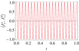
Figure 1: Behavior of the average value of $J_{x}^{a,b}$ for $\Lambda_{a}=\Lambda_{b}$ (units of energy), $\Lambda_{ab}=2.13$, $K_{a}=K_{b}=10.$ and initial conditions $\langle J_{x}^{a}\rangle(0)=\langle J_{x}^{b}\rangle(0)=1.$, $\langle J_{y}^{a,b}\rangle(0)=0$. The time is expressed in units of energy/$\hbar$.

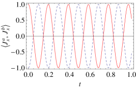
Figure 2: Behavior of the average value of $J_{x}^{a,b}$ for $\Lambda_{a}=\Lambda_{b}$ (units of energy), $\Lambda_{ab}=2.13$, $K_{a}=10.,K_{b}=10.$ and initial conditions $\langle J_{x}^{a}\rangle(0)=1,\langle J_{x}^{b}\rangle(0)=-1.$, $\langle J_{y}^{a,b}\rangle(0)=0$. The time is expressed in units of energy/$\hbar$.

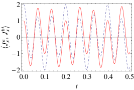
Figure 3: Behavior of the average value of $J_{x}^{a,b}$ for $\Lambda_{a}=\Lambda_{b}$ (units of energy), $\Lambda_{ab}=0.8$, $K_{a}=10.,K_{b}=10.$ and initial conditions $\langle J_{x}^{a}\rangle(0)=1.$,$\langle J_{x}^{b}\rangle(0)=2.$, $\langle J_{y}^{a,b}\rangle(0)=0$. The time is expressed in units of energy/$\hbar$.

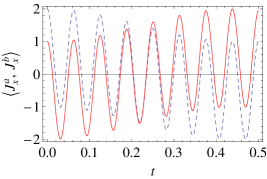
Figure 4: Behavior of the average value of $J_{x}^{a,b}$ for $\Lambda_{a}=\Lambda_{b}$ (units of energy), $\Lambda_{ab}=1.$, $K_{a}=10.,K_{b}=10.$ and initial conditions $\langle J_{x}^{a}\rangle(0)=1.$,$\langle J_{x}^{b}\rangle(0)=2.$, $\langle J_{y}^{a,b}\rangle(0)=0$. The time is expressed in units of energy/$\hbar$.

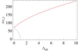
Figure 5: Behavior of $\omega_{1}(t)$ (dashed line) and $\omega_{2}(t)$ (straight line) for $\Lambda_{a}=\Lambda_{b}$ (units of energy).

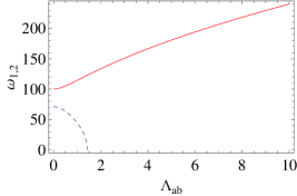
Figure 6: Behavior of $\omega_{1}(t)$ (dashed line) and $\omega_{2}(t)$ (straight line) for $\Lambda_{a}=2\Lambda_{b}$ (units of energy).

A few comments on the dynamics of the system are in order here. Compared to our previous analysisnoi1 , the present analysis does not allow the study of long-time scale phenomena since their detection is abruptly increased with $N$, thus only short-time scale effects are reliable. Furthermore we point out that the dynamics should become aperiodic in the general case.

When the initial state is a coherent spin state for each species, $\left|\psi\left(0\right)\right\rangle=\left|\psi\left(0\right)\right\rangle_{a}\left|\psi\left(0\right)\right\rangle_{b}$, where $\left|\psi\left(0\right)\right\rangle_{i}=C_{i}\sum_{m_{i}=-N_{i}/2}^{N_{i}/2}\sqrt{\frac{N_{i}!}{\left(\frac{N_{i}}{2}+m_{i}\right)!\left(\frac{N_{i}}{2}-m_{i}\right)!}}\tan^{m_{i}}\left(\frac{\theta_{i}}{2}\right)e^{-im_{i}\phi_{i}}\left|m_{i}\right\rangle$, $C_{i}=\sin^{N_{i}/2}\left(\frac{\theta_{i}}{2}\right)\cos^{N_{i}/2}\left(\frac{\theta_{i}}{2}\right)e^{-i\frac{N_{i}}{2}\phi_{i}}$, $i=a,b$, then the initial conditions are:

$\left\langle J_{x}^{a}\right\rangle\left(0\right)=-\frac{N_{a}}{2}\cos\theta_{a}$, $\left\langle J_{x}^{b}\right\rangle\left(0\right)=-\frac{N_{b}}{2}\cos\theta_{b}$, $\left\langle J_{y}^{a}\right\rangle\left(0\right)=\frac{N_{a}}{2}\sin\theta_{a}\sin\phi_{a}$, $\left\langle J_{y}^{b}\right\rangle\left(0\right)=\frac{N_{b}}{2}\sin\theta_{b}\sin\phi_{b}$.

In this case the same type of behavior, as for the small imbalance, is observed. In Fig. 7 we take the values $\theta_{a}=\theta_{b}=\pi/2.$ and $\phi_{a}=\phi_{b}=\pi/4.$

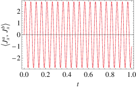
Figure 7: Behavior of the average value of $J_{x}^{a,b}$ for $\Lambda_{a}=\Lambda_{b}$ (units of energy), $\Lambda_{ab}=2.13$ and initial conditions with $N_{a}=N_{b}=100.$ and $\theta_{a}=\theta_{b}=\pi/2.$ and $\phi_{a}=\phi_{b}=\pi/4.$. The time is expressed in units of energy/$\hbar$.

The quantum dynamics above investigated could be experimentally reproduced. If we refer for instance to the mixture of ${}^{85}Rb$ and ${}^{87}Rb$ atoms realized by the JILA group exp6 , a wide tuning of s-wave interactions is possible via Feshbach resonances. In particular it is possible to fix the scattering length of ${}^{87}Rb$ and to tune the scattering length of ${}^{85}Rb$ as well as the interspecies one. That allows one to explore the parameter space in a wide range and to realize the symmetric regime $\Lambda_{a}=\Lambda_{b}=\Lambda$ as well as the asymmetric one. Furthermore one can tune the inter well coupling, i. e. the parameters $K_{a},K_{b}$, in such a way to get the semiclassical limit. Another possible realization of the phenomena above described could be obtained with the mixture of ${}^{41}K$ and ${}^{87}Rb$ atoms produced by the LENS group exp5 , which offers a wide possibility of driving from the weak to the strong interacting regime because of the presence of several magnetic Feshbach resonances simoni .

V Semiclassical dynamics

In this Section we briefly introduce the semiclassical limit of our model within the linear approximation in order to make a comparison with the quantum results obtained above. A detailed semiclassical analysis has been already carried out in the recent literature (see Refs. mix1 ; mix2 ; mix3 ; mix4 ; mix4bis ). Here we only recall the classical equations of motion to give a physical interpretation of $q_{a,b}$ and $p_{a,b}$ in Eq. (14). From the Hamiltonian (9), we can derive the following equations of motion for the components of the vectors: $\overrightarrow{J}^{a,b}$:

$$\frac{dJ^{a}_{x}}{dt} = -\Lambda_{a}J_{y}^{a}J_{z}^{a}-\Lambda_{ab}J_{y}^{a}J_{z}^{b},$$ (43)

$$\frac{dJ^{b}_{x}}{dt} = -\Lambda_{b}J_{y}^{b}J_{z}^{b}-\Lambda_{ab}J_{y}^{b}J_{z}^{a},$$ (44)

$$\frac{dJ^{a}_{y}}{dt} = \Lambda_{a}J_{x}^{a}J_{z}^{a}+\Lambda_{ab}J_{x}^{a}J_{z}^{b}+K_{a}J_{z}^{a},$$ (45)

$$\frac{dJ^{b}_{y}}{dt} = \Lambda_{a}J_{x}^{b}J_{z}^{b}+\Lambda_{ab}J_{x}^{b}J_{z}^{a}+K_{b}J_{z}^{b},$$ (46)

$$\frac{dJ^{a}_{z}}{dt} = -K_{a}J_{y}^{a},$$ (47)

$$\frac{dJ^{b}_{z}}{dt} = -K_{b}J_{b}^{a}.$$ (48)

These equations imply that $(\overrightarrow{J}^{a})^{2}=(J^{a}_{x})^{2}+(J^{a}_{y})^{2}+(J^{a}_{z})^{2}$ and $(\overrightarrow{J}^{b})^{2}=(J^{b}_{x})^{2}+(J^{b}_{y})^{2}+(J^{b}_{z})^{2}$ are constants, so we can introduce:

$$J_{x}^{a}=||J^{a}||\sin\theta_{a}\cos\varphi_{a},J_{y}^{a}=||J^{a}||\sin\theta_{a}\sin\varphi_{a},J_{z}^{a}=||J^{a}||\cos\theta_{a},$$ (49)

and:

$$J_{x}^{b}=||J^{b}||\sin\theta_{b}\cos\varphi_{b},J_{y}^{b}=||J^{b}||\sin\theta_{b}\sin\varphi_{b},J_{z}^{b}=||J^{b}||\cos\theta_{b}.$$ (50)

Using (49) and (50) in (43)-(48), we obtain the equationsmix3 :

$$\frac{d\theta_{a}}{dt} = K_{a}\sin\varphi_{a},$$ (51)

$$\frac{d\theta_{b}}{dt} = K_{b}\sin\varphi_{b},$$ (52)

$$\frac{d\varphi_{a}}{dt} = (\Lambda_{a}J^{a}\cos\theta_{a}+\Lambda_{ab}J^{b}\cos\theta_{b})+K_{a}\cot\theta_{a}\cos\varphi_{a},$$ (53)

$$\frac{d\varphi_{b}}{dt} = (\Lambda_{b}J^{b}\cos\theta_{b}+\Lambda_{ab}J^{a}\cos\theta_{a})+K_{b}\cot\theta_{b}\cos\varphi_{b}.$$ (54)

These equations coincide with Eqs. (5)-(8) in Ref. mix3 and Eqs. (5) in Ref.mix4bis and Eqs. (3) in Ref.mix4 . The energy conservation introduces one extra constraint, so that the phase space is actually three-dimensional. This may permit in certain conditions the observation of classical chaos. If we linearize the Equations (51)-(54) around the point $\theta_{a}=\theta_{b}=\pi/2,\varphi_{a}=\varphi_{b}=0$, we find the equations of motion:

$$\frac{d\delta\theta_{a}}{dt} = K_{a}\varphi_{a},$$ (55)

$$\frac{d\delta\theta_{b}}{dt} = K_{b}\varphi_{b},$$ (56)

$$\frac{d\varphi_{a}}{dt} = -(\Lambda_{a}J^{a}\delta\theta_{a}+\Lambda_{ab}J^{b}\delta\theta_{b})-K_{a}\delta\theta_{a},$$ (57)

$$\frac{d\varphi_{b}}{dt} = -(\Lambda_{b}J^{b}\delta\theta_{b}+\Lambda_{ab}J^{a}\delta\theta_{a})-K_{b}\delta\theta_{b},$$ (58)

where $\theta_{a}=\pi/2+\delta\theta_{a}$ and $\theta_{b}=\pi/2+\delta\theta_{b}$. These equations derive from the Hamiltonian:

$$H_{eff}=K_{a}J^{a}\frac{\varphi_{a}^{2}}{2}+K_{b}J^{b}\frac{\varphi_{b}^{2}}{2}+\frac{1}{2}\left[(\Lambda_{a}(J^{a})^{2}+K_{a}J^{a})(\delta\theta_{a})^{2}+(\Lambda_{b}(J^{b})^{2}+K_{b}J^{b})(\delta\theta_{a})^{2}+2\Lambda_{ab}J^{a}J^{b}\delta\theta_{a}\delta\theta_{b}\right],$$ (59)

with the Poisson brackets, $\{\varphi_{a},J^{a}\delta\theta_{a}\}=1$ and $\{\varphi_{b},J^{b}\delta\theta_{b}\}=1$. By rescaling the variable $\varphi_{i}$ and $\delta\theta_{i}$ ($i=a,b$) as $\varphi_{i}\rightarrow\frac{1}{\sqrt{J^{a}K_{a}}}\tilde{\varphi_{i}}$ and $\delta\theta_{i}\rightarrow\sqrt{J^{a}K_{a}}\delta\tilde{\theta_{i}}$, we do obtain the corresponding classical hamiltonian of (16), with Poisson brackets $\{\tilde{\varphi_{i}},J^{i}\delta\tilde{\theta_{i}}\}=1$. This Hamiltonian can be diagonalized in a standard way by introducing a linear combination of the variables $\tilde{\varphi_{i}}$ and $\delta\tilde{\theta_{i}}$ that preserves the Poisson brackets. The diagonalized Hamiltonian will be that of two independent classical harmonic oscillators of variables $\varphi_{1},\varphi_{2}$ and $\delta\theta_{1},\delta\theta_{2}$. Applying then the Bohr-Sommerfeld quantization we do reobtain the spectrum (31), giving the desired connection between the semiclassical and the quantum approach. This leads also to a physical interpretation of the conjugate variables $q_{a,b}$ and $p_{a,b}$ in Eq. (14) as the azimuthal angles of the pseudospins $\overrightarrow{J}^{a,b}$. The full classical solution of Eqs. (51)-(54) can be found in Refs. mix1 ; mix2 ; mix3 ; mix4 ; mix4bis .

VI Conclusions and perspectives

In this paper we investigated the quantum dynamics of a Bose Josephson junction made of a binary mixture of BECs loaded in a double well potential within the two-mode approximation. Focussing on the regime where the number of atoms is very large, a mapping onto a $SU(2)$ spin problem together with a Holstein-Primakoff transformation has been performed to calculate the time evolution of the imbalance between the two wells. This approach allows one to exactly solve the system under the assumption of weak interatomic interactions. The results show an instability towards a phase-separation above a critical positive value of the interspecies interaction while the system evolves towards a coherent tunneling regime for negative interspecies interactions. The detection of a phase separation could be experimentally achieved in current experiments with a mixture of ${}^{85}Rb$ and ${}^{87}Rb$ atomsexp6 .

We point out that all the above results are obtained within the linear approximation. It would be interesting to extend our model beyond the linear regime; in such a case the classical dynamics may exhibit a chaotic behavior in some parameter range because the phase-space is three dimensional. At the quantum level, these features will show up in the spectrum as well as the eigenstates of the Hamiltonian. Indeed the Hamiltonian is not time reversal invariant because of the terms linear in $J_{x}/J_{z}$, and we expect that the distribution of spacings between energy levels should follow the GUE (Gaussian Unitary ensemble) statistics mehta . Regarding the dynamics, we conjecture that the short time scale behavior of the quantum system will look chaotic, but the long time behavior will not. Such an analysis will be carried out in detail in a forthcoming publication.

Appendix A Coefficients

The coefficients $a^{{}^{\prime}}$, $b^{{}^{\prime}}$, $a^{{}^{{}^{\prime\prime}}}$, $b^{{}^{\prime\prime}}$ are defined as follows:

$$a^{{}^{\prime}} = \frac{2\omega_{ab}}{\sqrt{4\omega_{ab}^{2}+\left[\left(\omega_{b}^{2}-\omega_{a}^{2}\right)+\sqrt{\left(\omega_{a}^{2}-\omega_{b}^{2}\right)^{2}+4\omega_{ab}^{2}}\right]^{2}}},$$ (60)

$$b^{{}^{\prime}} = \frac{\left(\omega_{b}^{2}-\omega_{a}^{2}\right)+\sqrt{\left(\omega_{a}^{2}-\omega_{b}^{2}\right)^{2}+4\omega_{ab}^{2}}}{\sqrt{4\omega_{ab}^{2}+\left[\left(\omega_{b}^{2}-\omega_{a}^{2}\right)+\sqrt{\left(\omega_{a}^{2}-\omega_{b}^{2}\right)^{2}+4\omega_{ab}^{2}}\right]^{2}}},$$ (61)

$$a^{{}^{\prime\prime}} = \frac{2\omega_{ab}}{\sqrt{4\omega_{ab}^{2}+\left[\left(\omega_{b}^{2}-\omega_{a}^{2}\right)-\sqrt{\left(\omega_{a}^{2}-\omega_{b}^{2}\right)^{2}+4\omega_{ab}^{2}}\right]^{2}}},$$ (62)

$$b^{{}^{\prime\prime}} = \frac{\left(\omega_{b}^{2}-\omega_{a}^{2}\right)-\sqrt{\left(\omega_{a}^{2}-\omega_{b}^{2}\right)^{2}+4\omega_{ab}^{2}}}{\sqrt{4\omega_{ab}^{2}+\left[\left(\omega_{b}^{2}-\omega_{a}^{2}\right)-\sqrt{\left(\omega_{a}^{2}-\omega_{b}^{2}\right)^{2}+4\omega_{ab}^{2}}\right]^{2}}}.$$ (63)

References

• (1) A. J. Leggett, Rev. Mod. Phys. 73 (2001) 307.
• (2) S. Inouye, M. R. Andrews, J. Stenger, H. J. Miesner, D. M. Staper-Kurn, W. Ketterle, Nature 392 (1998) 151.
• (3) B. Paredes, A. Widera, V. Murg, O. Mandel, S. Folling, J. I. Cirac, G. V. Shlyapnikov, T. W. Hansch, I. Bloch, Nature 429 (2004) 377.
• (4) D. Jaksch, C. Bruder, J. I. Cirac, C. W. Gardiner, P. Zoller, Phys. Rev. Lett. 81 (1998) 3108; M. Greiner, O. Mandel, T. Esslinger, T. W. Hansch, I. Bloch, Nature 415 (2002) 39.
• (5) G. Kalosakas, A. R. Bishop, Phys. Rev. A 65 (2002) 043616; G. Kalosakas, A. R. Bishop, V. M. Kenkre, Phys. Rev. A 68 (2003) 023602.
• (6) R. Gati, M. K. Oberthaler, J. Phys. B: At. Mol. Opt. 40 (2007) R61.
• (7) G. Ferrini, A. Minguzzi, F. W. J. Hekking, Phys. Rev. A 78 (2008) 023606.
• (8) J. Javanainen, Phys. Rev. Lett. 57 (1986) 3164; I. Zapata, F. Sols, A. J. Leggett, Phys. Rev. A 57 (1998) 1050.
• (9) A. Smerzi, S. Fantoni, S. Giovanazzi, S. R. Shenoy, Phys. Rev. Lett. 79 (1997) 4950; S. Raghavan, A. Smerzi, S. Fantoni, S. R. Shenoy, Phys. Rev. A 59 (1999) 620.
• (10) S. Giovanazzi, A. Smerzi, S. Fantoni, Phys. Rev. Lett. 84 (2000) 4521.
• (11) F. S. Cataliotti, S. Burger, C. Fort, P. Maddaloni, F. Minardi, A. Trombettoni, M. Inguscio, Science 293 (2001) 843.
• (12) M. Albiez, R. Gati, J. Folling, S. Hunsmann, M. Cristiani, M. K. Oberthaler, Phys. Rev. Lett. 95 (2005) 010402.
• (13) S. Levy, E. Lahoud, I. Shomroni, J. Steinhauer, Nature 449 (2007) 579.
• (14) D. M. Stamper-Kurn, H. J. Misner, A. P. Chikkaur, S. Inouye, J. Stenger, W. Ketterle, Phys. Rev. Lett. 83 (1999) 661; M. R. Matthews, B. P. Anderson, P. C. Haljan, D. S. Hall, M. J. Holland, J. E. Williams, C. E. Wieman, E. A. Cornell, Phys. Rev. Lett. 83 (1999) 3358; M. Mudrich, S. Kraft, K. Singer, R. Grimm, A. Mosk, M. Weidemuller, Phys. Rev. Lett. 88 (2002) 253001.
• (15) G. Modugno, G. Ferrari, G. Roati, R. J. Brecha, A. Simoni, M. Inguscio, Science 294 (2001) 1320; G. Modugno, M. Modugno, F. Riboli, G. Roati, M. Inguscio, Phys. Rev. Lett. 89 (2002) 190404; G. Thalhammer, G. Barontini, L. De Sarlo, J. Catani, F. Minardi, M. Inguscio, Phys. Rev. Lett. 100 (2008) 210402.
• (16) S. B. Papp, C. E. Wieman, Phys. Rev. Lett. 97 (2006) 180404; S. B. Papp, J. M. Pino, C. E. Wieman, Phys. Rev. Lett. 101 (2008) 040402.
• (17) S. Ashhab, C. Lobo, Phys. Rev. A 66 (2002) 013609; H. Pu, W. Zhang, P. Meystre, Phys. Rev. Lett. 89 (2002) 090401; K. Molmer, Phys. Rev. Lett. 90 (2003) 110403.
• (18) G. Mazzarella, M. Moratti, L. Salasnich, M. Salerno, F. Toigo, J. Phys. B: At. Mol. Opt. 42 (2009) 125301; G. Mazzarella, M. Moratti, L. Salasnich, F. Toigo, J. Phys. B: At. Mol. Opt. 43 (2010) 065303.
• (19) X. Q. Xu, L. H. Lu, Y. Q. Li, Phys. Rev. A 78 (2008) 043609.
• (20) I. I. Satija, R. Balakrishnan, P. Naudus, J. Heward, M. Edwards, C. W. Clark, Phys. Rev. A 79 (2009) 033616.
• (21) B. Julia-Diaz, M. Guilleumas, M. Lewenstein, A. Polls, A. Sanpera, Phys. Rev. A 80 (2009) 023616.
• (22) M. Guilleumas, B. Julia-Diaz, M. Mele-Messeguer, A. Polls, Las. Phys. 20 (2010) 1163.
• (23) C. Wang, P. G. Kevrekidis, N. Whitaker, B. A. Malomed, Physica D 327 (2008) 2922.
• (24) B. Sun, M. S. Pindzola, Phys. Rev. A 80 (2009) 033616.
• (25) A. Naddeo, R. Citro, J. Phys. B: At. Mol. Opt. 43 (2010) 135302.
• (26) T. Holstein, H. Primakoff, Phys. Rev. 58 (1949) 1098.
• (27) M. P. Strzys, J. R. Anglin, Phys. Rev. A 81 (2010) 043616.
• (28) H. T. Ng, P. T. Leung, Phys. Rev. A 71 (2005) 013601.
• (29) G. J. Milburn, J. Corney, E. M. Wright, D. F. Walls, Phys. Rev. A 55 (1997) 4318.
• (30) D. Ananikian, T. Bergeman, Phys. Rev. A 74 (2006) 039905.
• (31) H. J. Lipkin, N. Meshkov, A. J. Glick, Nucl. Phys. 62 (1965) 188; N. Meshkov, A. J. Glick, H. J. Lipkin, Nucl. Phys. 62 (1965) 199; A. J. Glick, H. J. Lipkin, N. Meshkov, Nucl. Phys. 62 (1965) 211.
• (32) S. Dusuel, J. Vidal, Phys. Rev. B 71 (2005) 224420; P. Ribeiro, J. Vidal, R. Mosseri, Phys. Rev. Lett. 99 (2007) 050402; R. Orus, S. Dusuel, J. Vidal, Phys. Rev. Lett. 101 (2008) 025701.
• (33) A. Simoni, F. Ferlaino, G. Roati, G. Modugno, M. Inguscio, Phys. Rev. Lett. 90 (2003) 163202.
• (34) M. L. Mehta, Random Matrices, Elsevier/Academic Press, Amsterdam, 2005.