Matching factors for four-quark operators in schemes
Abstract
The non-perturbative renormalization of four-quark operators plays a significant role in lattice studies of flavor physics. For this purpose, we define regularization-independent symmetric momentum-subtraction () schemes for flavor-changing four-quark operators and provide one-loop matching factors to the scheme in naive dimensional regularization. The mixing of two-quark operators is discussed in terms of two different classes of schemes. We provide a compact expression for the finite one-loop amplitudes which allows for a straightforward definition of further schemes.
I Introduction
The study of physical processes which change the strangeness by one unit (), such as the decay of a kaon into two pions, is important for the understanding of CP violation within the Standard Model (SM) and its possible extensions. Such processes can be used to measure the parameter of direct CP violation , to study the rule, and to calculate long-distance contributions to mixing and the parameter of indirect CP violation Noaki:2001un ; Blum:2001xb ; Buras:2003zz ; Buras:2010pza ; Christ:2010gi . The resulting constraints for the Cabibbo-Kobayashi-Maskawa (CKM) matrix elements allow for a precise test of the SM. The weak interaction which mediates these processes with change in the strangeness can be described by local four-fermion operators at low energy scales, where the character of the vector boson interaction is essentially point like, see Refs. Vainshtein:1975sv ; Witten:1975bh ; Shifman:1975tn ; Witten:1976kx ; Gilman:1979bc and Refs. Buchalla:1995vs ; Buras:1998raa ; Buras:2011we for reviews. Matrix elements which describe, e.g., two-pion decays of kaons can then be computed with the help of lattice simulations.
In order to perform the renormalization of relevant operators in the lattice computation one can adopt a renormalization scheme which is independent of the regulator. Such a scheme can then be implemented in both non-perturbative lattice calculations and continuum perturbation theory. This allows for a conversion of lattice results to the modified minimal subtraction () scheme which is not directly applicable in lattice simulations. In Ref. Martinelli:1994ty the non-perturbative renormalization (NPR) technique and regularization independent (RI) momentum-subtraction schemes were defined for this purpose.
In the context of light up, down, and strange quark-mass determinations quark bilinear operators need to be studied for the NPR procedure. The required matching factors which convert the quark masses and fields from the RI schemes to the scheme are known up to three-loop order Martinelli:1994ty ; Franco:1998bm ; Chetyrkin:1999pq ; Gracey:2003yr in perturbative Quantum Chromodynamics (QCD). The renormalization constants in these regularization independent momentum-subtraction () schemes are determined at an exceptional momentum point of the considered amplitude. In the case of the quark bilinear operators the exceptional momentum configuration is distinguished by the fact that no momentum leaves the operator. However, a lattice simulation with an exceptional momentum configuration for the renormalization constants is more disposed to effects of chiral symmetry breaking Aoki:2007xm . Furthermore, in the scheme unwanted infrared effects exist and the matching factors show a poor convergence behavior. For these reasons a non-exceptional momentum configuration was proposed in Ref. Aoki:2007xm and the framework and concepts of new schemes with a symmetric subtraction point were worked out in Ref. Sturm:2009kb . The symmetric subtraction point is characterized by the fact that a momentum leaves the inserted operator.
The matching factors for the conversion of quark masses from the schemes with a symmetric subtraction point to the scheme were computed to two-loop order Sturm:2009kb ; Gorbahn:2010bf ; Almeida:2010ns ; Gracey:2011fb by considering the amputated Green’s functions with insertion of the scalar or pseudo-scalar operator. These schemes exhibit a better infrared behavior, and also the coefficients of the perturbative expansion of the matching factors are smaller. Therefore their use led to a significant reduction of the systematic uncertainties in the light quark mass determinations following this approach Aoki:2010dy compared to previous studies, see Ref. Allton:2008pn .
For the insertion of any multi-quark operator into an amputated Green’s function the fermion field for each external leg needs to be renormalized. In Ref. Sturm:2009kb two schemes, the and scheme, were suggested for the renormalization with a symmetric subtraction point. It was also shown that the former is equivalent to the scheme and is thus known to three-loop order Martinelli:1994ty ; Chetyrkin:1999pq ; Gracey:2003yr , whereas the latter is known to two-loop order Sturm:2009kb ; Almeida:2010ns ; Gorbahn:2010bf ; Gracey:2011fb . The corresponding calculation requires the computation of amputated Green’s functions with insertion of the vector or axial-vector operator and the utilization of Ward-Takahashi-identities.
We would like to mention that also the tensor operator has applications in lattice simulations, see, e.g., Ref. Donnellan:2007xr and a scheme with a symmetric subtraction point has been introduced in Ref. Sturm:2009kb . Its matching factor and anomalous dimension is known to two-loop order Sturm:2009kb ; Almeida:2010ns ; Gracey:2011fb . Also moments of twist-2 operators used in deep inelastic scattering have been studied in a scheme in Refs. Gracey:2010ci ; Gracey:2011zn .
In view of these successes and advantages, the definition has been extended to flavor-changing four-quark operators in Ref. Aoki:2010pe , where the one-loop QCD corrections to different matching factors have been computed, and also the anomalous dimensions were provided. These results were then used for the determination of the parameter which is needed to parametrize the hadronic matrix element for the theoretical description of mixing. For the case of an exceptional subtraction point the matching factors were determined at next-to-leading order in Refs. Ciuchini:1997bw ; Buras:2000if based on Ref. Donini:1995xj . Similarly the matching for flavor-changing four-quark operators with an exceptional subtraction point was determined in Refs. Ciuchini:1995cd ; Buras:2000if . The purpose of this paper is to introduce schemes with a non-exceptional subtraction point for flavor-changing four-quark operators as well as to provide the corresponding matching factors for the conversion from these schemes to the scheme in naive dimensional regularization (). To this end we first present the framework needed to properly take into account the mixing with two-quark operators which was not needed in the case. We then study the insertion of the operators into amputated Green’s functions in perturbative QCD at one-loop order to determine the renormalization constants.
The outline of this work is as follows. In Sec. II we define the set of four-quark operators used in this work. In Sec. III we discuss some generalities of the renormalization of the operators in the scheme as well as in a general scheme and introduce our notation. In Sec. IV we provide a classification of projectors used to define the schemes and present our results for the finite one-loop amplitude as well as conversion factors from different schemes to the scheme. Finally we close with a summary and conclusions in Sec. V.
II The bases of operators
In this section we define operator bases of the effective Hamiltonian of electroweak interactions, where we closely follow the notation of Ref. Buras:1993dy . We work in an effective three-flavor theory including the up, down, and strange quark. This effective theory is valid for energies below the charm quark mass. The effective Hamiltonian reads
| (1) |
with Fermi coupling constant and renormalization scale . The symbols denote Wilson coefficients and are four-quark operators, which we will discuss in terms of “physical” and “chiral” operator bases in different schemes labeled . In the case of the physical operator bases the effective Hamiltonian is expressed in terms of ten operators which are grouped into current-current operators, QCD penguin operators, and electroweak penguin operators. The physical operator bases are classified by the physical origin of their respective operators, whereas the chiral operator basis is classified by irreducible representations of the chiral symmetry.
II.1 The physical bases
Let us start with the traditional physical operator basis of Refs. Gilman:1979bc ; Gilman:1982ap ; Buras:1992tc ; Ciuchini:1993vr . The current-current operators are defined by
| (2) |
the QCD penguin operators are defined by
| (3) |
the electroweak penguin operators are defined by
| (4) |
with , , and
| (5) |
where refers to the spinor structure , and are color indices, and , , and are the fields of the up, down, and strange quarks. This basis of operators is referred to as “basis I” in the following. Alternatively we can Fierz transform and to
| (6) |
The basis of operators is called “basis II” in the following. Operators with color contractions as in are called color diagonal, operators with color contractions as in are called color mixed. It will also be useful to define the Fierz transformation of , i.e.,
| (7) |
In an explicit four-dimensional regularization scheme, such as lattice regularization, and can be used interchangeably. In dimensional regularization, however, the contribution of evanescent operators such as
| (8) |
has to be included. The evanescent operators vanish at tree level if the regulator is removed, see, e.g., Refs. Buras:1989xd ; Dugan:1990df ; Buras:1992tc ; Herrlich:1994kh .
II.2 The chiral basis
The operators are not linearly independent, i.e., one can eliminate three operators by expressing them as linear combinations of the remaining ones. In a regularization which breaks Fierz transformations also evanescent operators enter these relations. The reduced operator basis of linearly independent operators can then be classified according to irreducible representations of and flavor symmetries Vainshtein:1975sv ; Shifman:1975tn , and the resulting operator basis will be referred to as the “chiral basis” in the following. The linear independence of its elements will become important later for the non-perturbative definition of RI schemes with the help of projectors.
We proceed along the lines of Ref. Blum:2001xb amending their discussion by the contributions of evanescent operators since we work in dimensional regularization. We first eliminate the operators , , and using
| (9) |
The remaining seven operators can then be recombined according to irreducible representations of the chiral flavor-symmetry group . The details of this decomposition including evanescent operators are given in App. A. The chiral operator basis is thus given by
| (10) |
where denotes the respective irreducible representation of . Instead of expressing Eqs. (II.2) and (II.2) in terms of the operators of basis I and evanescent operators we could have also eliminated the latter by introducing the operators , of basis II and with the help of Eq. (8).
III Renormalization
In this section we discuss the renormalization of the four-quark operators starting with some generalities concerning operator renormalization at fixed gauge. We then describe the one-loop off-shell renormalization of the operators in the different bases in the scheme in detail and provide a discussion of renormalization in a general scheme. A brief discussion of some details concerning the Wilson coefficients of the chiral basis concludes this section.
III.1 Renormalization at fixed gauge
The renormalization schemes described in this work are defined at a fixed covariant gauge with gauge fixing parameter , where () corresponds to the Landau (Feynman) gauge. The gauge-fixing procedure explicitly breaks the gauge symmetry, and it can be shown that mixing with three classes of operators can occur KlubergStern:1975hc ; Joglekar:1975nu ; Deans:1978wn ; Collins:1984xc ; Buras:1992tc ; Dawson:1997ic : (i) gauge-invariant operators which do not vanish using the equations of motion, (ii) gauge-invariant operators which vanish using the equations of motion, and (iii) gauge non-invariant operators which are either BRST invariant or vanish using the equations of motion.
In a general renormalization scheme , a renormalized four-quark operator can be written as
| (11) |
where are the bare four-quark operators, are evanescent operators, () are gauge-invariant (gauge non-invariant) operators involving only two quark fields. The symbols , , , and denote renormalization constants. The sum over the respective operator basis for , , , and is implied. The operators belong to class (i), the operators belong to class (i) or (ii), and the operators belong to class (iii). Operators of class (ii) and (iii) do not contribute to physical amplitudes KlubergStern:1975hc ; Joglekar:1975nu ; Deans:1978wn ; Collins:1984xc . The mixing of operators can be avoided by using the background field gauge Buras:1992tc ; Ciuchini:1993vr ; Abbott:1980hw .
III.2 The scheme
In the following we discuss the off-shell renormalization of the operators in the scheme with massless quarks at one-loop order in perturbative QCD. We use naive dimensional regularization () in space-time dimensions with a naive anti-commutation definition of . For multi-loop calculations the operator basis of Ref. Chetyrkin:1997gb is more convenient and allows for a straightforward treatment of . Since we restrict ourselves in this work to the one-loop order, we adhere to the traditional bases in order to connect with previous works in this field. The -renormalization of the four-quark operators with a focus on on-shell renormalization is discussed, e.g., in Refs. Gilman:1979bc ; Wise:1980qb at one loop and in Refs. Buras:1992tc ; Ciuchini:1993vr at two-loop order.
The four-quark operators are of mass-dimension , so that in the massless limit mixing can only occur with operators , , and of mass-dimension . For off-shell external states the operator
| (12) |
mixes under renormalization with the operators at the one-loop level Buras:1992tc ; Wise:1979at . This operator is of class (i), i.e., it is nonzero in the limit of on-shell external states. In this limit, however, the operator becomes linearly dependent on the four-quark operators , and one finds Gilman:1979bc ; Wise:1979at ; Buras:1992tc
| (13) |
with
| (14) |
At one-loop order the renormalized operator in the scheme is given by
| (15) |
with
| (16) |
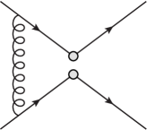
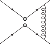
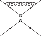
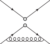
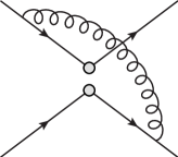
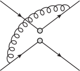
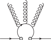
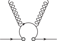
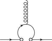
There are two different types of diagrams that need to be considered: current-current diagrams, where each fermion line involving a quark field of the operator extends to the external quark fields, and penguin diagrams, where one fermion line involving quark fields of the operator begins and ends at the operator. We depict the corresponding one-loop diagrams in Fig. 1 and Fig. 2. The one-loop current-current diagrams determine the mixing of the four-quark operators with themselves (given in ), while the penguin diagrams determine the mixing of with the four-quark operators (given in ).
We first consider the off-shell renormalization of operator basis I and II. The current-current contributions in separate in blocks given by Gilman:1979bc ; Wise:1980qb ; Buras:1992tc ; Ciuchini:1993vr
 |
 |
 |
 |
 |
 |
| (17) |
and
| (18) |
where the subscripts , of denote that the matrix acts on the space of operators and . This notation is also used for other block-diagonal matrices in the remainder of this section. The matrix is identical for basis I and II.
The penguin contributions in are given by
| (19) |
for basis I and II. For on-shell matrix elements we use Eq. (13) in Eq. (15) and thus reproduce the results for the anomalous dimensions of Refs. Gilman:1979bc ; Wise:1980qb ; Buras:1992tc ; Ciuchini:1993vr .
The set of evanescent operators used in Eq. (15) to define the scheme consists of operators
| (20) |
and
| (21) |
as well as
| (22) |
and
| (23) |
and finally
| (24) |
where , and and are color indices. The explicit contributions of order are determined by the “Greek” method Tracas:1982gp in accordance with two-loop calculations such as Ref. Buras:2000if . For operator basis I we have . The renormalization coefficients of the evanescent operators in Eq. (15) decompose in blocks and are given by
| (25) |
for basis I. Similarly for basis II we have , and one obtains
| (26) |
If operators transform in an irreducible representation of a given symmetry, they only mix with other operators transforming in the same irreducible representation. In the case of the chiral basis the decomposition of operators according to irreducible representations of is given in Eqs. (II.2). The set of operators used in Eq. (15) for the chiral basis is given by and , where the operators , , and are defined in Eq. (8). The matrix is then again block-diagonal with
| (27) |
and
| (28) |
The nonzero elements of are given in Tab. 1. In the chiral basis the on-shell limit of is given by
| (29) |
III.3 Regularization-independent schemes - The mixing of four-quark operators
In the following we define schemes for the four-quark operator bases. The schemes are defined non-perturbatively, so that they can be used in lattice simulations as well as in continuum perturbation theory. In lattice calculations the schemes serve as intermediate schemes and allow for a straightforward conversion of the studied quantity to the scheme. In this subsection we focus on the mixing of four-quark operators among themselves. In terms of Eq. (11) this means that we provide the renormalization conditions to determine the renormalization matrix . The renormalization conditions which determine the mixing of two-quark operators and with the four-quark operators , i.e., and , are discussed in subsection III.4. While the content of this subsection thus suffices to define the schemes for the and operators of the chiral basis, the discussion of subsection III.4 is necessary to complete the schemes for the operators.
Let us consider a set of bare operators that is closed under renormalization and contains the set of four-quark operators , i.e., . The renormalized operators in the or an scheme can be expressed in terms of the bare operators by
| (30) |
The renormalization conditions of the schemes are formulated in terms of renormalized amputated Green’s functions with a single insertion of such an operator , where denotes the wave function renormalization scheme and indicates the external states of the Green’s function. In this subsection we only consider Green’s functions with four external quarks which we denote by .
The renormalized amputated Green’s function is related to the bare amputated Green’s function by
| (31) |
where is the quark wave function renormalization constant, which relates the bare quark field to the renormalized quark field in the scheme .
Various wave function renormalization schemes have been proposed in Ref. Sturm:2009kb and will be used later. In order to convert the quark fields from the scheme to the scheme matching factors
| (32) |
have been computed with .
The operators which are renormalized in an scheme can be converted to the scheme
| (33) |
using the conversion matrix
| (34) |
The renormalization matrix has been discussed in the previous Sec. III.2, whereas the matrix is determined by the renormalization conditions of the scheme. Using Eqs. (32) and (34) one can express Eq. (31) completely in terms of matching factors and renormalized Green’s functions
| (35) |
In our case the set of operators is given by , where are the four-quark operators of basis I, II, or the chiral basis and are the corresponding evanescent operators used to define the scheme in the previous section. Since the evanescent operators are an artifact of dimensional regularization and escape a regularization-independent definition, their contribution to the right-hand side of Eq. (33) should be avoided. In order to achieve this, one defines new subtracted operators from the set of bare operators .
In general for any regulator one first has to subtract all contributions specific to the regularization from a given bare operator. Hence, in dimensional regularization we perform modified minimal subtraction of the evanescent operators Ciuchini:1995cd ; Donini:1995xj , i.e., the subtracted operator is defined as
| (36) |
where is chosen such that it cancels all contributions of proportional to a pole in . In principle the choice of evanescent operators used on the right-hand side of Eq. (36) is not unique. A useful choice is the basis given in the previous section to define the scheme for operator basis I, II, and the chiral basis, and for which we therefore have
| (37) |
For convenience we adopt this definition of the subtracted operator in the following. In a lattice regularization one has to perform a similar subtraction of lower-dimensional two-quark operators Blum:2001xb which do not occur in dimensional regularization. From now on we only consider such subtracted operators and therefore drop the explicit notation of the superscript “”.
In the schemes one imposes the renormalization condition Martinelli:1994ty that amputated Green’s functions with given off-shell external states at a given momentum point and in a fixed gauge coincide with their tree-level value. This condition is made explicit by choosing a certain set of projectors in spinor, color, and flavor space that is applied to the four-quark amputated Green’s function and imposing
| (38) |
where denotes the insertion of the operator in the amputated Green’s function at tree level. Since we are only interested in -renormalized operators , we do not provide conditions for the operators and in this work. For a set of operators we will provide projectors to determine the elements of the renormalization matrix . If no two-quark operators mix with the four-quark operators , i.e., and in Eq. (11), the renormalization matrix is given by Blum:2001xb
| (39) |
where
| (40) |
and . If two-quark operators mix with the operators , Eq. (39) has to be modified slightly, which is discussed in subsection III.4.
The matrix given in Eq. (39) depends on the regulator used to define the scheme, i.e., the matrix obtained using a lattice regulator is different from the matrix obtained in dimensional regularization. The condition of Eq. (38), however, fixes the physical amplitudes of the -renormalized operators at a certain off-shell momentum point to its tree-level value, which is independent of the choice of the regulator. Therefore, the physical amplitudes of the -renormalized operators agree for all choices of the regulator.
We define the scheme in the limit of vanishing quark masses. The choice of projectors , the gauge fixing, and the momentum configuration of the off-shell amputated Green’s functions defines the scheme up to mixing with two-quark operators. The explicit form of the projectors will be discussed later in Sec. IV. Note that Eq. (38) matches the amputated Green’s function of a certain physical process with insertion of operators at a certain off-shell momentum point.
In particular for the operators we consider the off-shell amputated Green’s functions of the process
| (41) |
with quarks , momenta , , , , color indices , and spinor indices , , , . Using crossing symmetry we could equally well consider the scattering amplitude
| (42) |
The momentum configuration used in Eq. (38) to define the scheme is then given by
| (43) |
with
| (44) |
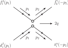
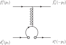
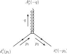
in Minkowski space, where is the subtraction scale. This momentum configuration and our convention for open indices for the amputated Green’s functions is shown in Fig. 3. In Fig. 4 we explicitly show the corresponding penguin diagrams at one-loop order, where a momentum transfer leaves the operator. This choice of momenta is non-exceptional (no partial sum of incoming external momenta vanishes) which has the advantage of suppressing unwanted infrared effects in the lattice simulation.
 |
 |
In Ref. Ciuchini:1995cd a scheme was defined which uses exceptional kinematics and a different momentum point for current-current and penguin diagrams, see Fig. 5 of Ref. Ciuchini:1995cd . The momentum configuration in the scheme is given by at for current-current diagrams and and at for penguin diagrams. We consider the scheme in the following for completeness, illustration, and check of our calculation. Another scheme with exceptional kinematics which uses the same momentum point for current-current and penguin diagrams is discussed in Ref. Liu:2011zzz .
III.4 Regularization-independent schemes - The mixing of two-quark operators
In the following we discuss the mixing of the two-quark operators and with the four-quark operators in the schemes. Such mixing occurs, e.g., for the operators of the chiral basis. The two-quark operators mix through the penguin diagrams, and therefore their mixing should be determined from amplitudes which only receive contributions from penguin-type contractions.
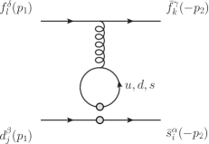
Two kinds of such amplitudes will be considered in the following: (a) amputated Green’s functions with two external quarks and one external gluon and (b) amputated Green’s functions with four external quarks corresponding to the process , where the quark flavor . The momentum flow and our convention for open indices in case (a) is shown in Fig. 5. The corresponding momenta , , and for the scheme satisfy Eq. (44). This momentum configuration is also non-exceptional. In case (b) we adhere to the momentum configuration and choice of indices shown in Figs. 3 and 4. In the following we define the schemes in such a way that both cases, (a) and (b), lead to identical one-loop conversion factors from the scheme to the scheme. At higher loops, however, the schemes defined by (a) differ from the schemes defined by (b). Case (b) can be implemented in lattice simulations in a straightforward way Blum:2001xb , while case (a) requires an external gluonic state. Nevertheless, the availability of both cases should be beneficial for lattice simulations, in particular to estimate higher-loop effects that are neglected in this work.
Case (a) is formulated in terms of renormalized amputated Green’s functions which are related to the bare amputated Green’s functions by
| (45) |
where is the gluon wave function renormalization constant, which relates the bare gluon field to the renormalized gluon field in the scheme . Using Eqs. (32) and (34) one can express Eq. (45) as
| (46) |
We then determine the renormalization coefficients and by imposing
| (47) |
for a certain set of projectors . Since only tree-level insertions of and need to be considered in this work, we do not provide renormalization conditions to define -renormalized operators and . The definition of schemes for the two-quark operators and is beyond the scope of this work.
The conditions given in Eqs. (38) and (47) then allow for a non-perturbative determination of the renormalization matrices , , and defined in Eq. (11). Without loss of generality we set in the following. We find
| (48) |
with
| (49) |
and
| (50) |
Case (b) is formulated in terms of the renormalized amputated Green’s function corresponding to the process that is shown in Fig. 4 at one loop. Note that the quark flavor for as opposed to for which was used in subsection III.3. We then determine the mixing of the two-quark operators by imposing
| (51) |
for a certain set of projectors . The renormalization coefficients for case (b) can be obtained from Eqs. (III.4) and (49) by replacing with
| (52) |
We provide the explicit projectors used to define the schemes in Sec. IV. We will define the set of projectors and such that the resulting schemes agree at one loop. From now on we refer to schemes defined using case (a) as schemes, while we do not write a subscript for schemes defined using case (b).
Since in the physical application of the scheme one is not interested in the conversion of the operators and from the scheme to the scheme, it is useful to decompose the matrix of Eq. (34) into several blocks. The conversion relation of Eq. (33) for subtracted operators is then given by
| (53) |
where the operators are either of basis I, II, or the chiral basis. The three blocks , , and are obtained by imposing the renormalization condition of Eqs. (38) and (47), i.e., we have to evaluate with off-shell external legs, see Eq. (35).
We denote on-shell matrix elements of the operators with a general external momentum setting by for which one finds
| (54) |
since the on-shell matrix elements of the two-quark operators and are related to the on-shell matrix elements of . At the one-loop level only the two-quark operator contributes to the right-hand side of Eq. (III.4), and one has
| (55) |
In Sec. IV we compute and as well as the on-shell conversion factors
| (56) |
at one loop for different schemes and for operator basis I, II, and the chiral basis.
III.5 The Wilson coefficients of the chiral basis
For lattice calculations it is advantageous to consider the chiral operator basis that uses the classification of operators according to irreducible representations of the chiral symmetry. In this basis the operators of each irreducible representation can be renormalized independently. Therefore the effective Hamiltonian should be expressed in terms of the operators .
On-shell matrix elements of the effective Hamiltonian defined in Eq. (1) in terms of read
| (57) |
where is the renormalization scale and is the conversion matrix of Eq. (54) for the chiral basis. The Wilson coefficients are, however, typically given for the traditional operator bases in Refs. Altarelli:1980fi ; Buras:1991jm ; Buras:1993dy ; Ciuchini:1993vr . Therefore it remains to relate the above Wilson coefficients to the known Wilson coefficients corresponding to the operators of basis I or II.
To this end we first note that Eqs. (II.2) and (II.2) hold for -renormalized operators without contributions of evanescent operators, i.e.,
| (58) |
with
| (59) |
where the matrix can be read off from Eqs. (II.2) and (II.2). This equation holds for the operators of basis I and II. Note that – are equal to –, see Eqs. (II.2), and therefore the respective sub-block in is proportional to the unit matrix. In the scheme, however, finite contributions of evanescent operators modify Eq. (58) to
| (60) |
at the one-loop level. The coefficients are given by
| (61) |
for operators of basis I and
| (62) |
for operators of basis II.
Since the Hamiltonian is independent of the choice of operator basis, we have
| (63) |
Therefore using Eqs. (60) and we can determine in
| (64) |
At one-loop order one finds Buras:1993dy
| (65) |
for the Wilson coefficients corresponding to basis I and
| (66) |
for the Wilson coefficients corresponding to basis II.
In App. B we give an alternative way to determine using our results for an scheme derived in the next section.
IV Calculation and Results
In the following we give the main results of this work. We first express the finite part of the amplitudes defined in Secs. III.3 and III.4 in a compact and instructive way in Sec. IV.1. We then discuss the general matching procedure in Sec. IV.2 before giving the conversion matrices for different and schemes in Secs. IV.3 and IV.4.
IV.1 A compact expression for the amplitudes
The schemes are defined by applying projectors in spinor, color, and flavor space to the renormalized amputated Green’s functions , see Eqs. (38), (47), and (51), and thus to , see Eqs. (35) and (III.4). In this section we calculate , , and as defined in Secs. III.3 and III.4. The diagrams are generated with the program QGRAF Nogueira:1991ex , and the symbolic manipulations are carried out using FORM Vermaseren:2000nd . We give results for the respective exceptional momentum configuration of the scheme as well as the non-exceptional momentum configuration of the schemes. We consider the operators of basis I, II, and the chiral basis.
We simplify the -renormalized amplitudes using the decomposition Buras:2000if
| (67) |
and the Fierz identities
| (68) | ||||
| (69) |
The resulting one-loop expressions are written as
| (70) | ||||
| (71) | ||||
| (72) |
where denotes the insertion of the operator of basis I, II or the chiral basis at tree level and the sum over repeated indices is implied. The operators are obtained from the operators by replacing the gamma structure with , i.e.,
| (73) |
for the case of and and analog for all other and . Similarly the operators are obtained from the operators by replacing the gamma structure with , i.e.,
| (74) |
for the case of and analog for all other . In Tabs. IV.1–4 we give the coefficients with at one loop for the chiral basis and the exceptional and non-exceptional momentum configuration. The corresponding results for basis I and II can be obtained from these tables using Eq. (60). The constant is defined as
| (75) |
where is the digamma function abramowitz+stegun .
In order to determine the conversion factors from the schemes to the scheme we need to study projected Green’s functions
| (76) |
where and both and have open spinor, color, and flavor indices. The action of on for is thus given by
| (77) |
with spinor indices , color indices , and flavor index , as shown in Fig. 3. Similarly
| (78) |
where is a Lorentz index and enumerates the generators of the algebra, see Fig. 5. The summation over repeated indices is implied. The resulting expression naturally depends on the choice of the projectors . In the following we make certain assumptions about the structure of the projectors, i.e., we discuss different classes of projectors. For each class of projectors we can then give a very compact form of the amputated Green’s function that can, without loss of generality, be used to calculate all projections of the respective class.
First we restrict the discussion to projectors which contain no external momentum, except for at most the external momentum
We also do not consider projectors that contain vectors such as , , , or which break Lorentz symmetry explicitly. The corresponding class of projectors shall be denoted by . We will also study the sub-class of projectors that additionally do not contain the external momentum .
Let us focus on the amputated Green’s functions with four external quarks and examine the projection of a spinor structure such as under projectors of class , i.e.,
where the two factors belong to the two fermion lines, and the combination contains strings of gamma matrices without remaining open Lorentz indices. Then the ansatz
| (79) |
with Lorentz indices and is justified by the Lorentz-transformation properties of both sides since does not contain any Lorentz vectors apart from the momentum . The coefficients and can be determined by contraction with and , respectively. We find
| (80) |
Therefore not all of the spinor structures that appear in the general amplitude of Eq. (IV.1) are independent under projection with , i.e.,
| (81) |
with . The resulting projected amputated Green’s functions for up to one-loop order can be written as
| (82) |
If we further restrict the discussion to projectors of the sub-class , we find
| (83) |
with using the same arguments as in Eq. (79) without the term proportional to . Therefore, for projectors of class and we can write
| (84) |
with , where we can read off the coefficients from Eq. (14) for basis I and II or from Eq. (III.2) for the chiral basis.
IV.2 The matching procedure
In the following sections we give the one-loop conversion coefficients from different schemes to the scheme. We first explain the general procedure of calculating the conversion coefficients and then give results for explicit and schemes.
At one loop the conversion from schemes to the scheme in terms of renormalized amputated Green’s functions reads
| (85) |
with wave function conversion factor for and for , see Eq. (III.4). In order to define the scheme, and hence to determine the coefficients and , we apply projectors to Eq. (IV.2) and use the conditions of Eqs. (38) and (47) for the schemes and of Eqs. (38) and (51) for the schemes, see Sec. III.4.
From Eqs. (71) and (72) and the conditions of Eqs. (47) and (51) we can already conclude that
| (86) |
is the only possible result at one loop. For convenience we provide a specific projector to determine the mixing of the two-quark operator . In an scheme, we can use
| (87) |
where is a generator of the group algebra and the convention of open indices is given in Fig. 5. In an scheme, we can use
| (88) |
At higher loops the additional operators Buras:1992tc
| (89) | ||||
with and possibly other non-gauge-invariant two-quark operators mix with the operators. We therefore need to provide additional renormalization conditions at higher loops in order to define the schemes for the operators uniquely, i.e., we need to specify additional projectors. The specific choice of projectors to determine the mixing with the operator and additional operators which occur at higher loops is not relevant for the one-loop conversion factors given in this work. At one loop the conversion factors can thus be given without specifying the details of higher-loop contributions.
In the following we use the , , and wave function renormalizations defined in Refs. Martinelli:1994ty ; Chetyrkin:1999pq ; Sturm:2009kb . The corresponding conversion factors up to one-loop order
| (90) |
are given by
| (91) |
for the and wave function renormalization schemes as well as
| (92) |
for the scheme.
IV.3 The and schemes
We first give the conversion coefficients for schemes that either (i) use only projectors of class or (ii) use the exceptional momentum configuration and projectors of class . The coefficients are already determined in Eq. (86), and it remains to obtain the coefficients by applying projectors to the amputated Green’s function .
In case (i) the amputated Green’s function simplifies to
| (93) |
under projectors , see Eq. (IV.1). This should be compared to Eq. (IV.2), i.e.,
| (94) |
where we used Eqs. (IV.1). If we impose the condition of Eq. (38) and insert Eq. (86), we find
| (95) |
with identity matrix .
In case (ii) we have , and therefore Eq. (IV.1) simplifies to
| (96) |
One can read off the conversion matrix by comparing Eq. (IV.2) to Eq. (IV.3) with
| (97) |
In both cases the conversion coefficients are unique up to the definition of the quark wave function renormalization . In other words, in these cases the details of the projectors do not matter, as long as one uses a sufficient number of independent projectors to determine all elements of the conversion matrices or -factors, respectively.
The choice of the wave function renormalization scheme only affects the diagonal elements of . One can also combine different wave function renormalization schemes with different schemes for the operators in a straightforward way using Eq. (IV.3).
We call the scheme of case (i) scheme, where corresponds to the wave function renormalization scheme and corresponds to the wave function renormalization scheme. The name reflects that we restrict the choice of projectors to the class .
The scheme corresponding to case (ii) is the scheme, and we give results only for the wave function renormalization.
In Tabs. IV.1–IV.1 we give the values for , which is defined in Eq. (56), for the scheme with wave function renormalization and operators of basis I, II, and the chiral basis. In Tabs. IV.1 and IV.1 we present the results for for the and the scheme and operators of the chiral basis.
We would like to point out that the result of Tab. IV.1 for and or agrees with the result of Ref. Ciuchini:1995cd for the conversion from the scheme to the scheme. In Ref. Buras:2000if the current-current contributions in the scheme have been considered. Our result for these contributions agrees with the one of Ref. Buras:2000if , which can be seen by using the results of Eq. (60) and Tab. IV.1 and combining them with the quark wave function renormalization constant of Eq. (5.3) of Ref. Buras:2000if .
Furthermore, the result for the operator in Tabs. IV.1 and IV.1 agrees with the result of Ref. Aoki:2010pe for the conversion from the and the scheme to the scheme for the (VV+AA)– operator.
IV.4 Results for the schemes
In the following we discuss the non-exceptional momentum configuration and schemes defined by projectors of the class . This allows for the definition of new and independent schemes which we call () schemes, where denotes the choice of the wave function renormalization scheme as in the previous section. We give results only for the chiral basis which does not contain linearly dependent operators. Since mixing only occurs within the blocks of the , , and operators, we renormalize each block separately.
We first note that for a scheme with projectors of the class the conversion matrices cannot be simply read off from Tabs. IV.1–4 due to the nonzero contribution of . This means that the schemes defined in this section, unlike the schemes discussed in the previous section IV.3, depend on the specific choice of the projectors. However, any non-degenerate linear transformation of a given set of projectors leaves the conversion matrix of Eq. (34) invariant. We give the projectors used to define the schemes in the following. The projectors will be expressed in terms of
| (98) |
where all indices are as shown in Fig. 3.
The operator only mixes with itself, so we only need to provide a single projector . We adopt the and schemes defined in Ref. Aoki:2010pe so that for the operator we use
| (99) |
The operators and also only mix with themselves under renormalization, and therefore we have to provide two projectors. We choose
| (100) |
with the property
| (101) |
The one-loop mixing coefficients for the operators shall be determined using the projectors
| (102) |
where
| (103) |
Other choices of projectors within class , which are not linear combinations of the projectors given above, are possible and might lead to smaller conversion factors and a better convergence of the perturbative expansion. The reader can easily obtain the respective projections using the results which we provide in Tabs. IV.1–4.
In Tabs. IV.1 and IV.1 we provide the resulting one-loop conversion matrices for the and schemes. We note that the result for the operator agrees with the result of Ref. Aoki:2010pe for the conversion of the (VV+AA)– operator. In Tabs. IV.1–IV.1 we give the individual conversion matrices for the operators in the same schemes.
IV.5 Discussion
In the previous sections we provided results for the conversion from different and schemes to the scheme. In general the different schemes have a different magnitude of one-loop corrections and a different rate of convergence of the perturbative expansion of in . In the context of lattice QCD and non-perturbative renormalization it is thus useful to have several schemes to choose from in order to estimate the effects of missing higher-order terms in the perturbative expansion. In this work we give four different schemes for each operator of the chiral operator basis.
Since we only give one-loop results, we cannot estimate the rate of convergence of the different schemes presented in this paper. In some cases where higher-order results in schemes are known, such as the conversion relation for light quark mass determinations, the convergence in the schemes is significantly faster than the convergence in the traditional schemes.
It is, however, interesting to compare the magnitude of the one-loop corrections of different schemes. In Tab. IV.5 we give the spectral matrix norm and the maximum norm for the conversion matrices at and for the different blocks of operators in the chiral basis. The spectral norm of matrix is defined as the maximum singular value of the matrix and the maximum norm of matrix is defined as the maximum absolute value of the matrix elements. Therefore the spectral norm gives a good estimate of the general magnitude of the one-loop corrections since it is invariant under a change of operator basis. The maximum norm gives a good estimate of especially large individual mixing coefficients.
One observes that for the operator the one-loop coefficients for the scheme with wave function renormalization are of order , while the results vary from order to order . The schemes with have especially small one-loop coefficients. In this case the spectral norm is, of course, equal to the maximum norm. For the operators the spectral norm and the maximum norm for the scheme and the schemes is approximately twice the size of the schemes. In the case of the operators the maximum norm as well as the spectral norm in the scheme is significantly larger than the respective norm in the schemes. The difference is especially pronounced for the scheme.
We conclude that the magnitude of the one-loop contributions to varies significantly between the different schemes, and we expect that the same holds for the rate of convergence of the perturbative expansion of in . Note that Tab. IV.5 only gives the numerical values for Landau gauge and that the qualitative analysis of this section may be different for other gauges.
& (27,1) 2.45482 (27,1) 0.21184 (27,1) 0.45482 (27,1) 2.21184 (8,1) 10.61021 9.20457 (8,1) 5.34301 3.88889 (8,1) 5.21189 3.88889 (8,1) 12.03242 8.69111 (8,1) 11.17384 6.02444 (8,8) 11.42390 10.87124 (8,8) 3.23249 2.62348 (8,8) 4.77841 4.49561 (8,8) 1.62236 1.49561 (8,8) 4.26036 4.16227
V Summary and conclusion
Physical processes that change the strangeness by one unit play an important role in the field of flavor phenomenology. These processes can be studied in lattice simulations using an effective Hamiltonian of electroweak interactions that is formulated in terms of flavor-changing four-quark operators. In order to renormalize these operators non-perturbatively and to convert measured matrix elements to the scheme it is necessary to define renormalization schemes that are independent of the specific regulator. In this work we define renormalization schemes for different operator bases and provide one-loop matching factors to the scheme.
Since the different schemes project out different components of the perturbative series, the variety of schemes can be used to estimate the effects of higher-order corrections to the conversion matrices which are presently unknown. In this work we define four different schemes for each operator. We also provide a compact expression for the finite one-loop amplitudes that can be used by the reader to define further schemes in a straightforward way.
The numerical size of the one-loop contributions to the matching factors is discussed briefly for different schemes in the Landau gauge. We find that their magnitude varies significantly between the different and schemes.
In future work two-loop conversion factors will be calculated which will further reduce the systematic uncertainties in lattice calculations involving the effective Hamiltonian of electroweak interactions.
Acknowledgements.
We would like to thank the RBC/UKQCD collaboration, especially N.H. Christ, N. Garron, T. Izubuchi, R.D. Mawhinney, C.T. Sachrajda, and A. Soni, for many interesting and inspiring discussions. C.L. acknowledges support from the RIKEN FPR program. C.S. was partially supported by U.S. DOE under Contract No. DE-AC02-98CH10886.Appendix A Flavor and isospin decomposition of four-quark operators
In this appendix we give the flavor and isospin decomposition of the four-quark operators defined in Eqs. (II.1)-(5). We proceed along the lines of App. B of Ref. Blum:2001xb , carefully avoiding the use of Fierz transformations. We can then convert operators to operators including the evanescent operators of Eq. (8).
A.1 Left-left operators
The left-left operators can be written as
| (104) |
with left-handed quark fields and flavor indices , , , . We identify with an up quark, with a down quark, and with a strange quark. The color and spinor contractions are denoted by . The individual quark fields transform in the fundamental representation of , i.e., under we find
| (105) |
with
| (106) |
This transformation corresponds to the 81-dimensional representation of . We can decompose the tensor of this -dimensional representation as
| (107) |
where for a general tensor we have and . It is straightforward to check that the respective subspaces are invariant under Eq. (106) and that their dimensionality is given by
| (108) | ||||||
| (109) |
Since is symmetric under simultaneous exchange of we only need to consider the completely symmetric case and the completely antisymmetric case .
We can further decompose the remaining subspaces by considering the trace of a pair of upper and lower indices. If such a trace vanishes, it also vanishes after applying the transformation of Eq. (106), and therefore such a constraint defines an invariant subspace. For the completely symmetric case we distinguish between
| (110) | ||||||||
| (111) | ||||||||
| (112) |
where we sum over repeated indices. The subspace (i) has nine constraints and is thus -dimensional, the subspace (ii) is orthogonal to (i) and has one constraint and is thus -dimensional, and the remaining subspace (iii) is -dimensional. Therefore the completely symmetric case can be decomposed as
For the completely antisymmetric case the analog definition of subspaces leads to a zero-dimensional space (i), a -dimensional space (ii), and a -dimensional space (iii), i.e., the completely antisymmetric case can be decomposed as
This completes the classification of the left-left operators of the form given in Eq. (104) according to representations of . From now on we restrict the discussion to with either (I) exactly one field or (II) exactly one or field. In the case (I) only the elements and with are nonzero. Therefore they live in a -dimensional representation of isospin, and we can classify them according to irreducible isospin representations in the following. In the completely symmetric case (which is especially symmetric in ) they live in a -dimensional isospin representation, and we distinguish between
| (113) | |||||
| (114) |
where we sum over . The subspace (Ia) has two constraints and is thus -dimensional (), the subspace (Ib) is orthogonal to (Ia) and is thus -dimensional (). In the completely antisymmetric case lives in a -dimensional isospin representation. The respective subspace (Ia) has two constraints and is thus zero-dimensional, the respective subspace (Ib) is orthogonal to (Ia) and is thus two-dimensional (). In the case (II) the tensor transforms in the fundamental isospin representation ().
In the remainder of this subsection we give a list of left-left operators with transforming in irreducible representations of and isospin in which the operator
| (115) |
enters. The completely symmetric operators are given by
| (116) |
where indicates the representation of , and () indicates the isospin. The completely antisymmetric operator is given by
| (117) |
A.2 Left-right operators
The left-right operators can be written as
| (118) |
with right-handed quark fields . The individual quark fields transform in the fundamental representation of , i.e., under and we find
| (119) |
with
| (120) |
This transformation corresponds to the 9-dimensional representations of and . These -dimensional representations can be decomposed in a -dimensional subspace with vanishing trace of left (right) indices and in a -dimensional subspace with nonzero trace, i.e.,
| (121) |
This completes the classification of the left-right operators of the form given in Eq. (118) according to representations of . From now on we restrict the discussion to with only for (I) and or (II) , . The classification according to irreducible representations of isospin now follows from the analog discussion of left-left operators.
In the remainder of this subsection we give a list of left-right operators with transforming in irreducible representations of and isospin in which the operator
| (122) |
enters. It is straightforward to see that and transform in the representation of and in isospin representation , i.e., we define
| (123) |
Operators symmetric under are given by
| (124) |
One can also construct an operator that is antisymmetric under for with well-defined transformation under flavor and isospin:
| (125) |
A.3 Change of basis
Operators of the physical basis I and II with spinor structure – can be decomposed in the color-diagonal operators of Eqs. (A.1) and (117). We find
| (126) | ||||
| (127) | ||||
| (128) |
for the color-diagonal operators and
| (129) | ||||
| (130) | ||||
| (131) |
for the color-mixed operators with
| (132) |
Operators with spinor structure – are already in explicit and representations, i.e.,
| (133) | ||||
| (134) | ||||
| (135) |
with
| (136) | ||||
| (137) |
Appendix B Alternative determination of
In this appendix we provide an alternative method to determine defined in Eq. (64) relating the Wilson coefficients of the -renormalized operator basis I, II to the respective coefficients of the chiral basis.
To this end we consider an arbitrary scheme and express on-shell matrix elements of the effective Hamiltonian in terms of operators and first in terms of Wilson coefficients ,
| (138) |
and then in terms of Wilson coefficients ,
| (139) |
Since these equations hold for an arbitrary matrix element, we find
| (140) |
where is defined in Eq. (58). A comparison with Eq. (64) yields
| (141) |
Note that the left-hand side is just a conversion factor of Wilson coefficients in the scheme, and thus the right-hand side must also be independent of the scheme used to calculate and .
We calculate using Eq. (141) for the non-exceptional momentum configuration with projectors
| (142) | ||||
| (143) | ||||
| (144) | ||||
| (145) | ||||
| (146) | ||||
| (147) | ||||
| (148) |
with
| (149) |
This choice of projectors recovers the conversion matrices of the schemes for the non-exceptional momentum configuration. It makes use of projectors with a more complex flavor structure which allows for a definition of this scheme without considering each irreducible representation of operators separately. We use the basis of projectors with defined in Eqs. (IV.4). The details of the wave function renormalization given in drop out in Eq. (141) and hence we do not need to specify the wave function renormalization scheme . The result for using this method agrees with given in Sec. III.5.
References
- (1) J. I. Noaki et al. (CP-PACS), Phys. Rev. D68, 014501 (2003), arXiv:hep-lat/0108013
- (2) T. Blum et al. (RBC), Phys. Rev. D68, 114506 (2003), arXiv:hep-lat/0110075
- (3) A. J. Buras and M. Jamin, JHEP 01, 048 (2004), arXiv:hep-ph/0306217
- (4) A. J. Buras, D. Guadagnoli, and G. Isidori, Phys. Lett. B688, 309 (2010), arXiv:1002.3612 [hep-ph]
- (5) N. H. Christ (2010), arXiv:1012.6034 [hep-lat]
- (6) A. I. Vainshtein, V. I. Zakharov, and M. A. Shifman, JETP Lett. 22, 55 (1975)
- (7) E. Witten, Nucl. Phys. B104, 445 (1976)
- (8) M. A. Shifman, A. I. Vainshtein, and V. I. Zakharov, Nucl. Phys. B120, 316 (1977)
- (9) E. Witten, Nucl. Phys. B122, 109 (1977)
- (10) F. J. Gilman and M. B. Wise, Phys. Rev. D20, 2392 (1979)
- (11) G. Buchalla, A. J. Buras, and M. E. Lautenbacher, Rev. Mod. Phys. 68, 1125 (1996), arXiv:hep-ph/9512380
- (12) A. J. Buras (1998), arXiv:hep-ph/9806471
- (13) A. J. Buras (2011), arXiv:1102.5650 [hep-ph]
- (14) G. Martinelli, C. Pittori, C. T. Sachrajda, M. Testa, and A. Vladikas, Nucl. Phys. B445, 81 (1995), arXiv:hep-lat/9411010
- (15) E. Franco and V. Lubicz, Nucl. Phys. B531, 641 (1998), arXiv:hep-ph/9803491
- (16) K. G. Chetyrkin and A. Retey, Nucl. Phys. B583, 3 (2000), arXiv:hep-ph/9910332
- (17) J. A. Gracey, Nucl. Phys. B662, 247 (2003), arXiv:hep-ph/0304113
- (18) Y. Aoki et al., Phys. Rev. D78, 054510 (2008), arXiv:0712.1061 [hep-lat]
- (19) C. Sturm et al., Phys. Rev. D80, 014501 (2009), arXiv:0901.2599 [hep-ph]
- (20) M. Gorbahn and S. Jager, Phys. Rev. D82, 114001 (2010), arXiv:1004.3997 [hep-ph]
- (21) L. G. Almeida and C. Sturm, Phys. Rev. D82, 054017 (2010), arXiv:1004.4613 [hep-ph]
- (22) J. A. Gracey, Eur. Phys. J. C71, 1567 (2011), arXiv:1101.5266 [hep-ph]
- (23) Y. Aoki et al. (RBC) (2010), arXiv:1011.0892 [hep-lat]
- (24) C. Allton et al. (RBC-UKQCD), Phys. Rev. D78, 114509 (2008), arXiv:0804.0473 [hep-lat]
- (25) M. A. Donnellan et al., PoS LAT2007, 369 (2007), arXiv:0710.0869 [hep-lat]
- (26) J. A. Gracey, Phys. Rev. D83, 054024 (2011), arXiv:1009.3895 [hep-ph]
- (27) J. A. Gracey, JHEP 03, 109 (2011), arXiv:1103.2055 [hep-ph]
- (28) Y. Aoki et al. (2010), arXiv:1012.4178 [hep-lat]
- (29) M. Ciuchini et al., Nucl. Phys. B523, 501 (1998), arXiv:hep-ph/9711402
- (30) A. J. Buras, M. Misiak, and J. Urban, Nucl. Phys. B586, 397 (2000), arXiv:hep-ph/0005183
- (31) A. Donini, G. Martinelli, C. T. Sachrajda, M. Talevi, and A. Vladikas, Phys. Lett. B360, 83 (1995), arXiv:hep-lat/9508020
- (32) M. Ciuchini, E. Franco, G. Martinelli, L. Reina, and L. Silvestrini, Z. Phys. C68, 239 (1995), arXiv:hep-ph/9501265
- (33) A. J. Buras, M. Jamin, and M. E. Lautenbacher, Nucl. Phys. B408, 209 (1993), arXiv:hep-ph/9303284
- (34) F. J. Gilman and M. B. Wise, Phys. Rev. D27, 1128 (1983)
- (35) A. J. Buras, M. Jamin, M. E. Lautenbacher, and P. H. Weisz, Nucl. Phys. B400, 37 (1993), arXiv:hep-ph/9211304
- (36) M. Ciuchini, E. Franco, G. Martinelli, and L. Reina, Nucl. Phys. B415, 403 (1994), arXiv:hep-ph/9304257
- (37) A. J. Buras and P. H. Weisz, Nucl. Phys. B333, 66 (1990)
- (38) M. J. Dugan and B. Grinstein, Phys. Lett. B256, 239 (1991)
- (39) S. Herrlich and U. Nierste, Nucl. Phys. B455, 39 (1995), arXiv:hep-ph/9412375
- (40) H. Kluberg-Stern and J. B. Zuber, Phys. Rev. D12, 3159 (1975)
- (41) S. D. Joglekar and B. W. Lee, Ann. Phys. 97, 160 (1976)
- (42) W. S. Deans and J. A. Dixon, Phys. Rev. D18, 1113 (1978)
- (43) J. C. Collins, “Renormalization”, Cambridge, Uk: Univ. Pr. (1984) 380p
- (44) C. Dawson et al., Nucl. Phys. B514, 313 (1998), arXiv:hep-lat/9707009
- (45) L. F. Abbott, Nucl. Phys. B185, 189 (1981)
- (46) K. G. Chetyrkin, M. Misiak, and M. Munz, Nucl. Phys. B520, 279 (1998), arXiv:hep-ph/9711280
- (47) M. B. Wise, “Strong effects in weak nonleptonic decays”, (1980), SLAC-0227
- (48) M. B. Wise and E. Witten, Phys. Rev. D20, 1216 (1979)
- (49) N. Tracas and N. Vlachos, Phys. Lett. B115, 419 (1982)
- (50) T. Blum et al. (RBC-UKQCD) (2011), in preparation
- (51) G. Altarelli, G. Curci, G. Martinelli, and S. Petrarca, Nucl. Phys. B187, 461 (1981)
- (52) A. J. Buras, M. Jamin, M. E. Lautenbacher, and P. H. Weisz, Nucl. Phys. B370, 69 (1992)
- (53) P. Nogueira, J. Comput. Phys. 105, 279 (1993)
- (54) J. A. M. Vermaseren (2000), arXiv:math-ph/0010025
- (55) M. Abramowitz and I. A. Stegun, Handbook of Mathematical Functions with Formulas, Graphs, and Mathematical Tables, ninth Dover printing, tenth GPO printing ed. (Dover, New York, 1964) ISBN 0-486-61272-4