State sampling dependence of the Hopfield network inference

Abstract

The fully connected Hopfield network is inferred based on observed magnetizations and pairwise correlations. We present the system in the glassy phase with low temperature and high memory load. We find that the inference error is very sensitive to the form of state sampling. When a single state is sampled to compute magnetizations and correlations, the inference error is almost indistinguishable irrespective of the sampled state. However, the error can be greatly reduced if the data is collected with state transitions. Our result holds for different disorder samples and accounts for the previously observed large fluctuations of inference error at low temperatures.

I Introduction

The inverse Ising problem, also known as Boltzmann machine learning, is recently widely studied in the context of network inference. As we know, a large number of elements interacting with each other may yield collective behavior at the network level. Encouragingly, the pairwise Ising model was shown to be able to capture most of correlation structure in real neuronal networks Schneidman et al. (2006); Tang et al. (2008). The advent of techniques for multi-electrode recording or microarray measurement produces high throughput biological data. The inverse Ising problem tries to construct a statistical mechanics description of the original system directly from these data, which helps to better understand how the brain or other biological networks represent and process information Tkacik et al. (2010). On the other hand, to test proposed efficient inverse algorithms, one can alternatively collect the required data, i.e., magnetizations $\{m_{i}\}$ and two-point connected correlations $\{C_{ij}\}$($i,j$ run from $1$ to $N$ and $N$ is the number of elements in the network) from Monte Carlo simulations of a toy model Aurell et al. (2010); Marinari and Kerrebroeck (2010); Huang (2010a, b). Given the magnetizations and correlations, the underlying parameters (i.e., couplings and fields) of the pairwise Ising model are inferred to describe the statistics of the experimental data. In other words, the data is fitted with $P_{{\rm Ising}}(\boldsymbol{\sigma})\propto\exp\left[\sum_{i<j}J_{ij}\sigma_{i}\sigma_{j}+\sum_{i}h_{i}\sigma_{i}\right]$, such that the predicted magnetizations and correlations are consistent with those measured, i.e., $\left<\sigma_{i}\right>_{{\rm Ising}}=\left<\sigma_{i}\right>_{{\rm data}},\left<\sigma_{i}\sigma_{j}\right>_{{\rm Ising}}=\left<\sigma_{i}\sigma_{j}\right>_{{\rm data}}$. In this setting, we use $\boldsymbol{\sigma}$ to represent the configuration of the system and each component takes $\pm 1$. Previous studies along this line focused on the Sherrington-Kirkpatrick (SK) model Aurell et al. (2010); Marinari and Kerrebroeck (2010) and the Hopfield model Huang (2010a, b). However, the influence of state sampling on the network inference was overlooked and in this work, we will illustrate this most important issue on the fully connected Hopfield network reconstruction. We find that the quality of reconstruction depends on the way the data is collected via state samplings. A lazy Glauber dynamics can be easily trapped by a high-lying metastable state, however, in a finite system, it still has the possibility of a transition to a different state (free energy valley), provided that the amount of sampling time is chosen appropriately Billoire et al. (2011). If we present the system at low enough temperature $T$ and high memory load $\alpha$, these two different scenarios for state sampling will yield different qualities of network inference. The former maintains a high inference error regardless of which state we sample, while the latter reduces the error substantially.

The paper proceeds as follows. The fully connected Hopfield network is defined in Sec. II. We collect the data using a lazy Glauber dynamics and infer the network by message passing algorithm, which is also demonstrated in this section. Results and discussions are given in Sec. III. We conclude this paper in Sec. IV.

II Fully connected Hopfield network and its inference

The Hopfield network has been proposed in Refs. Hopfield (1982); Amit et al. (1985) as an abstraction of biological memory storage and was found to be able to store up to $0.144N$ random unbiased patterns Amit et al. (1987). If the stored patterns are dynamically stable, then the network is able to provide associative memory and its equilibrium behavior is described by the following Hamiltonian:

$$\mathcal{H}=-\sum_{i<j}J_{ij}\sigma_{i}\sigma_{j}$$ (1)

where $\sigma_{i}=+1$ indicates the spiking of neuron $i$ while $\sigma_{i}=-1$ means the silence. Coupling between neuron $i$ and $j$ is symmetric and constructed according to the Hebb’s rule:

$$J_{ij}=\frac{1}{N}\sum_{\mu=1}^{P}\xi_{i}^{\mu}\xi_{j}^{\mu}$$ (2)

where $\{\xi_{i}^{\mu}\}$ are $P$ stored patterns with each element $\xi_{i}^{\mu}$ taking $\pm 1$ with equal probability. These random stored patterns give rise to disorder leading to frustration in the low temperature. The ratio of the number of stored patterns to the network size $N$ is defined as the memory load $\alpha$, i.e., $\alpha\equiv\frac{P}{N}$.

Our prime concern is the study of the fully connected Hopfield network inference. In this network, each neuron is connected to all the other neurons and no self-interactions and external fields are assumed. The equilibrium properties of the fully connected Hopfield model has been addressed in Ref. Amit et al. (1987). In this work, we focus on the glassy phase which takes place when $T<T_{g}=1+\sqrt{\alpha}$. At all finite $\alpha$, this phase has a vanishing small overlap with any of the stored patterns. Furthermore, the replica symmetry solution for this phase is unstable and develops a hierarchically organized structure Amit et al. (1987); Tokita (1993) which leads to anomalously slow dynamic relaxation. The dynamics was shown to exhibit aging phenomena supporting the nontrivial structure of the phase space Montemurro et al. (2000). Therefore, starting from different initial configurations, the lazy Glauber dynamics will be trapped in different free energy valleys with high probability. For a finite system, free energy barriers around metastable states are always finite and the Glauber dynamics has the possibility to escape from local minima of free energy landscape. Therefore, as an inverse problem, we are interested in the influence of state sampling on the network inference in this phase, and we look at individual disorder samples with $N=125,\alpha=0.2$ in the low temperature $T=0.5$, and expect analysis on these individual disorder samples will provide valuable information on the state sampling dependence of the network inference for a general context.

To sample the state of the original model Eq. (1), we apply a lazy (non-optimized) Glauber dynamics rule:

$$P(\sigma_{i}\rightarrow-\sigma_{i})=\frac{1}{2}\left[1-\sigma_{i}\tanh\beta h_{i}\right]$$ (3)

where $\beta$ is the inverse temperature and $h_{i}=\sum_{j\neq i}J_{ij}\sigma_{j}$ is the local field neuron $i$ feels. In practice, we first randomly generate a configuration which is then updated by the local dynamics rule Eq. (3) in a randomly asynchronous fashion. In this setting, we define a Glauber dynamics step as $N$ proposed flips. As a lazy dynamics, we quench the system directly to the preset low temperature $T=0.5$ without any annealing schemes and run totally $4\times 10^{6}$ steps, among which the first $2\times 10^{6}$ steps are run for thermal equilibration and the other $2\times 10^{6}$ steps for computing magnetizations and correlations, i.e., ${m_{i}=\left<\sigma_{i}\right>_{{\rm data}},C_{ij}=\left<\sigma_{i}\sigma_{j}\right>_{{\rm data}}-m_{i}m_{j}}$ where $\left<\cdots\right>_{{\rm data}}$ denotes the average over the collected data. The state of the network is sampled every $100$ steps after thermal equilibration.

Given the measured magnetizations and correlations, we attempt to infer couplings via susceptibility propagation (SusProp) update rule Mézard and Mora (2009) which was shown to outperform other mean-field-type methods Huang (2010b). Before introducing this rule, we define two kinds of relevant messages. One is the cavity magnetization $m_{i\rightarrow j}$ of neuron $i$ in absence of neuron $j$; the other is the cavity susceptibility $g_{i\rightarrow j,k}$ which is the response of the cavity field $h_{i\rightarrow j}$ to the small change of the local field $h_{k}$ of neuron $k$. The SusProp rule can be derived using belief propagation plus fluctuation-response relation Huang (2010b) and is formulated as follows:

$$m_{i\rightarrow j} =\frac{m_{i}-m_{j\rightarrow i}\tanh J_{ij}}{1-m_{i}m_{j\rightarrow i}\tanh J_{ij}}$$ (4a)

$$g_{i\rightarrow j,k} =\delta_{ik}+\sum_{n\in\partial i\backslash j}\frac{1-m_{n\rightarrow i}^{2}}{1-(m_{n\rightarrow i}\tanh J_{ni})^{2}}\tanh J_{ni}g_{n\rightarrow i,k}$$ (4b)

$$J_{ij}^{{\rm new}} =\epsilon\left[\frac{1}{2}\log\left(\frac{(1+\widetilde{C_{ij}})(1-m_{i\rightarrow j}m_{j\rightarrow i})}{(1-\widetilde{C_{ij}})(1+m_{i\rightarrow j}m_{j\rightarrow i})}\right)\right]+(1-\epsilon)J_{ij}^{{\rm old}}$$ (4c)

$$\widetilde{C_{ij}} =\frac{C_{ij}-(1-m_{i}^{2})g_{i\rightarrow j,j}}{g_{j\rightarrow i,j}}+m_{i}m_{j}$$ (4d)

where $\partial i\backslash j$ denotes neighbors of neuron $i$ except $j$, $\delta_{ik}$ is the Kronecker delta function and $\epsilon(\in[0,1])$ is introduced as a damping factor and should be appropriately chosen to prevent the absolute updated $\tanh(J_{ij})$ from being larger than $1$. Note that all couplings in Eq. (4) have been scaled by the inverse temperature $\beta$.

To evaluate the reconstruction performance of SusProp, we define the inference error as $\Delta=\left[\frac{2}{N(N-1)}\sum_{i<j}(J_{ij}^{*}-J_{ij}^{{\rm true}})^{2}\right]^{1/2}$ where $J_{ij}^{*}$ is the inferred coupling while $J_{ij}^{{\rm true}}$ is the true one constructed according to Eq. (2). In Eq. (4), $\left(\{m_{i}\},\{C_{ij}\}\right)$ serve as inputs to the update rule. To run SusProp, we initially set all couplings to be zero and randomly initialize for every directed edge the message $m_{i\rightarrow j}\in[-1.0,1.0]$ and $g_{i\rightarrow j,k}=0$ if $i\neq k$ and $1.0$ otherwise. Then SusProp is iterated according to Eq. (4) until either all inferred couplings converge within a preset precision $\eta$ or the maximal number of iterations $\mathcal{T}_{max}$ is reached. In practice, we set $\mathcal{T}_{max}=3000,\eta=10^{-4}$ and $\epsilon$ varies from $\mathcal{O}(10^{-2})$ to $\mathcal{O}(10^{-4})$.

III Results and discussions

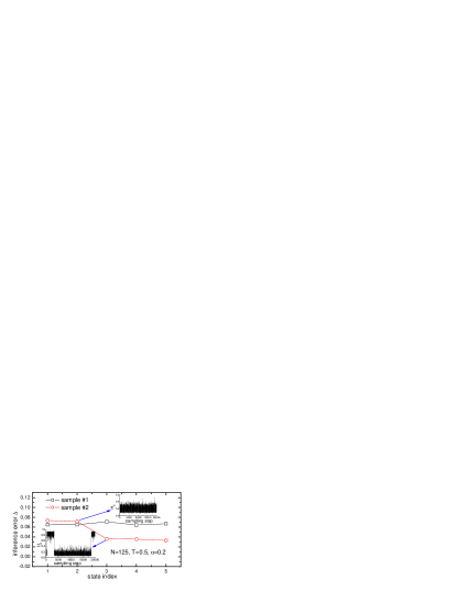
Figure 1: (Color online) State sampling dependence of the network inference. We present the inference error for two distinct disorder samples. For the second sample, the first two state samplings give large inference errors while the last three samplings reduce the error substantially. Insets give their corresponding evolutions of Hamming distances between the current sampled configuration and the first sampled one. For the first sample, all five state samplings provide nearly the same inference errors and their evolutions of the Hamming distances are similar to that of the second state sampling of the second sample. Note that the state index for the last three samplings of the second sample means different paths of multiple states sampling and that for the others means different states where the sampling is confined.

We simulate the fully connected Hopfield network of size $N=125$ at $T=0.5$ and $\alpha=0.2$ forcing the system to enter the glassy phase. The state sampling dependence of the network inference is illustrated in Fig. 1. To discriminate two kinds of scenarios for state sampling, we track the evolution of Hamming distance between current sampled configuration and the first sampled one. By Hamming distance, we mean $H_{d}=\frac{1}{2}\left(1-\frac{1}{N}\sum_{i=1}^{N}\sigma_{i}^{t}\sigma_{i}^{0}\right)$ where $\boldsymbol{\sigma}^{t}$ is the current sampled configuration while $\boldsymbol{\sigma}^{0}$ is the first sampled one. We also measure the energy for each sampled configuration during the whole state sampling process. For the lower inset of Fig. 1, the energy fluctuates around $-0.511$ with fluctuation of order $0.023$ while around $-0.510$ for the upper inset with nearly the same fluctuation amplitude. It can be seen clearly that the inference error depends strongly on the way the state is sampled, regardless of which state the lazy dynamics visits. In the first type, the sampling is confined in a single free energy valley, or the same level of the family tree like structure of the phase space Mézard et al. (1987); Tokita (1993). This case would probably occur since the limited amount of sampling time is not enough for the dynamics to escape from the current valley. Therefore, we observe one mean value of Hamming distance in the upper inset. Unfortunately, this type produces highly magnetized data especially at the low temperature, which gives rise to the non-convergence of SusProp and a high inference error. It should be emphasized that all samplings with the similar feature of Hamming distance evolution, as the upper inset shows, exhibit nearly the same inference error irrespective of the sample and the sampled state. In the second type, a transition to a different free energy valley or a higher level of phase space organization may happen due to the finiteness of the network if the temperature is not very low. We do observe this possibility in our simulations as the lower inset shows. In this case, another larger mean Hamming distance appears during the state sampling. Since each free energy valley is visited by the Glauber dynamics with a probability proportional to its thermodynamical weight Zhou (2007), when state transitions occur, the computed average of $\sigma_{i}\sigma_{j}$ or $\sigma_{i}$ over all $2\times 10^{4}$ sampled configurations amounts to the weighted sum, i.e., $\left<\sigma_{i}\sigma_{j}\right>_{{\rm data}}=\sum_{\gamma}w^{\gamma}\left<\sigma_{i}\sigma_{j}\right>_{\gamma},\left<\sigma_{i}\right>_{{\rm data}}=\sum_{\gamma}w^{\gamma}\left<\sigma_{i}\right>_{\gamma}$ where only a few states are considered depending on the actual state transitions in the sampling process and $\gamma$ is the state index the dynamics visits and $w^{\gamma}$ is the associated thermodynamical weight and proportional to the exponential of minus its scaled (by $\beta$) free energy Tokita (1993); Zhou and Li (2008). That is to say, we have now access to the correlations as well as magnetizations in the form of weighted sum. This weighted sum actually attenuates the high polarization of the supplied data and a relatively low inference error is achieved. In fact, SusProp converges in this case. For both types of state samplings, the result holds for other random samples, which accounts for the previously observed large fluctuations of inference error at low temperatures Huang (2010a, b).

Previous study Marinari and Kerrebroeck (2010) emphasized that the inference error can be drastically reduced by increasing the number of independent observations, which is consistent with our results in the sense that state transitions would occur with a higher probability if the number of sampling time increases. Importantly, our work discovered further that if the number of sampling time takes moderate values, the sampling with state transitions can reduce the inference error while the sampling without state transitions maintains a high inference error.

IV Conclusion

In conclusion, our study implies that, to lower the inference error, one should select the most efficient way to sample the system particularly when the phase space of the original model develops hierarchically organized structure and the amount of sampling time is limited (e.g, $2\times 10^{4}$ in our current simulations). Sampling with state transitions seems to be most effective to infer the finite-size network structure. In real neuronal networks, such as retinal network presented with natural movie stimuli, the coexistence of negative and positive couplings can lead to frustration and thus the emergence of many metastable states Tkacik et al. (2009); Mora and Bialek (2011). For instance, a recording from a salamander retina of $40$ neurons showed that several metastable states appear reproducibly across multiple presentations of the same movie Tkacik et al. (2009). Our result for the state sampling dependence of the Hopfield network inference may have some implications for the inference of real neuronal networks Schneidman et al. (2006); Stevenson et al. (2008); Cocco et al. (2009).

References

- Schneidman et al. (2006) E. Schneidman, M. J. Berry, R. Segev, and W. Bialek, Nature 440, 1007 (2006).
- Tang et al. (2008) A. Tang, D. Jackson, J. Hobbs, W. Chen, J. L. Smith, H. Patel, A. Prieto, D. Petrusca, M. I. Grivich, A. Sher, et al., J. Neurosci 28, 505 (2008).
- Tkacik et al. (2010) G. Tkacik, J. S. Prentice, V. Balasubramanian, and E. Schneidman, Proc. Natl. Acad. Sci. USA 107, 14419 (2010).
- Aurell et al. (2010) E. Aurell, C. Ollion, and Y. Roudi, Eur. Phys. J. B 77, 587 (2010).
- Marinari and Kerrebroeck (2010) E. Marinari and V. V. Kerrebroeck, J. Stat. Mech.: Theory Exp P02008 (2010).
- Huang (2010a) H. Huang, Phys. Rev. E 81, 036104 (2010a).
- Huang (2010b) H. Huang, Phys. Rev. E 82, 056111 (2010b).
- Billoire et al. (2011) A. Billoire, I. Kondor, J. Lukic, and E. Marinari, J. Stat. Mech.: Theory Exp p. P02009 (2011).
- Hopfield (1982) J. J. Hopfield, Proc. Natl. Acad. Sci. USA 79, 2554 (1982).
- Amit et al. (1985) D. J. Amit, H. Gutfreund, and H. Sompolinsky, Phys. Rev. Lett 55, 1530 (1985).
- Amit et al. (1987) D. J. Amit, H. Gutfreund, and H. Sompolinsky, Ann. Phys. 173, 30 (1987).
- Tokita (1993) K. Tokita, J. Phys. A 26, 6915 (1993).
- Montemurro et al. (2000) M. A. Montemurro, F. A. Tamarit, D. A. Stariolo, and S. A. Cannas, Phys. Rev. E 62, 5721 (2000).
- Mézard and Mora (2009) M. Mézard and T. Mora, J. Physiology Paris 103, 107 (2009).
- Mézard et al. (1987) M. Mézard, G. Parisi, and M. A. Virasoro, Spin Glass Theory and Beyond (World Scientific, Singapore, 1987).
- Zhou (2007) H. Zhou, Commun. Theor. Phys 48, 179 (2007).
- Zhou and Li (2008) H. Zhou and K. Li, Commun. Theor. Phys 49, 659 (2008).
- Tkacik et al. (2009) G. Tkacik, E. Schneidman, M. J. Berry, and W. Bialek (2009), e-print arXiv:0912.5409.
- Mora and Bialek (2011) T. Mora and W. Bialek, J. Stat. Phys 144, 268 (2011).
- Cocco et al. (2009) S. Cocco, S. Leibler, and R. Monasson, Proc. Natl. Acad. Sci. USA 106, 14058 (2009).
- Stevenson et al. (2008) I. H. Stevenson, J. M. Rebesco, L. E. Miller, and K. P. Körding, Current Opinion in Neurobiology 18, 582 (2008).