Serial Concatenation of RS Codes with Kite Codes: Performance Analysis, Iterative Decoding and Design

Abstract

In this paper, we propose a new ensemble of rateless forward error correction (FEC) codes. The proposed codes are serially concatenated codes with Reed-Solomon (RS) codes as outer codes and Kite codes as inner codes. The inner Kite codes are a special class of prefix rateless low-density parity-check (PRLDPC) codes, which can generate potentially infinite (or as many as required) random-like parity-check bits. The employment of RS codes as outer codes not only lowers down error-floors but also ensures (with high probability) the correctness of successfully decoded codewords. In addition to the conventional two-stage decoding, iterative decoding between the inner code and the outer code are also implemented to improve the performance further. The performance of the Kite codes under maximum likelihood (ML) decoding is analyzed by applying a refined Divsalar bound to the ensemble weight enumerating functions (WEF). We propose a simulation-based optimization method as well as density evolution (DE) using Gaussian approximations (GA) to design the Kite codes. Numerical results along with semi-analytic bounds show that the proposed codes can approach Shannon limits with extremely low error-floors. It is also shown by simulation that the proposed codes performs well within a wide range of signal-to-noise-ratios (SNRs).

I Introduction

Serially concatenated codes were first introduced by Forney [1]. A traditional concatenated code typically consists of an outer Reed-Solomon (RS) code, an inner convolutional code and a symbol interleaver in between. A typical example is the concatenation of an outer $\textrm{RS}[255,223,33]$ code and an inner convolutional code with rate 0.5 and constraint length 7, which has been adopted as the CCSDS Telemetry Standard [2]. The basic idea behind the concatenated codes is to build long codes from shorter codes with manageable decoding complexity. The task of the outer RS decoder is to improve the performance further by correcting “remaining” errors after the inner decoding. Since the invention of turbo codes [3] and the rediscovery of low-density parity-check (LDPC) codes [4], it has been suggested to use serially concatenated codes with outer RS codes and inner turbo/LDPC codes for data transmissions [5][6].

Binary linear rateless coding is an encoding method that can generate potentially infinite parity-check bits for any given fixed-length binary sequence. Fountain codes constitute a class of rateless codes, which were first mentioned in [7]. For a conventional channel code, coding rate is well defined; while for a Fountain code, coding rate is meaningless since the number of coded bits is potentially infinite and may be varying for different applications. The first practical realizations of Fountain codes were LT-codes invented by Luby [8]. LT-codes are linear rateless codes that transform $k$ information bits into infinite coded bits. Each coded bit is generated independently and randomly as a binary sum of several randomly selected information bits, where the randomness is governed by the so-called robust soliton distribution. LT-codes have encoding complexity of order $\log k$ per information bit on average. The complexity is further reduced by Shokrollahi using Raptor codes [9]. The basic idea behind Raptor codes is to precode the information bits prior to the application of an appropriate LT-code. For relations among random linear Fountain codes, LT-codes and Raptor codes and their applications over erasure channels, we refer the reader to [10].

Fountain codes were originally proposed for binary erasure channels (BECs). In addition to their success in erasure channels, Fountain codes have also been applied to other noisy binary input memoryless symmetric channels (BIMSCs) [11][12][13]. Comparing other noisy BIMSCs with BECs, we have the following observations.

1. Over erasure channels, Fountain codes can be used in an asynchronous way as follows. The transmission bits are first grouped into packets. Then LT-codes and/or Raptor codes are adapted to work in a packet-oriented way which is similar to the bit-oriented way. The only difference lies in that the encoders can insert a packet-head to each coded packet, specifying the involved information packets. While the receiver receives a coded packet, it also knows the connections of this coded packets to information packets. In this scenario, the receiver does not necessarily know the code structure before the transmission. The overhead due to the insertion of packet-head can be made negligible whenever the size of the packets is large. However, over other noisy channels, it should be more convenient and economic to consider only synchronous Fountain codes. This is equivalent to require that the receiver knows the structure of the code before transmission or shares common randomness with the transmitter. Otherwise, one must find ways to guarantee with probability 1 the correctness of the packet-head.

2. Both LT-codes and Raptor codes have been proved to be universally good for erasure channels in the sense that, no matter what the channel erasure probability is, the iterative belief propagation (BP) algorithm can recover the transmitted $k$ bits (packets) with high probability from any received $k(1+\epsilon)$ bits (packets). However, it has been proved [12] that no universal Raptor codes exist for BIMSCs other than erasure channels.

3. Over erasure channels, the receiver knows exactly when it successfully recovers the information bits and hence the right time to stop receiving coded bits. However, over other BIMSCs, no obvious ways (without feedback) exist to guarantee with probability 1 the correctness of the recovered information bits.

In this paper, we are concerned with the construction of synchronous rateless codes for binary input additive white Gaussian noise (BIAWGN) channels. We propose a new ensemble of rateless forward error correction (FEC) codes based on serially concatenated structure, which take RS codes as outer codes and Kite codes as inner codes. The inner Kite codes are a special class of prefix rateless low-density parity-check (PRLDPC) codes, which can generate as many as required random-like parity-check bits. The use of RS codes as outer codes not only lowers down error-floors but also ensures (with high probability) the correctness of successfully decoded codewords. The proposed codes may find applications in the following scenarios.

1. The proposed encoding method can definitely be utilized to construct FEC codes with any given coding rate. This feature is attractive for future deep-space communications [14].

2. The proposed codes can be considered as rate-compatible codes, which can be applied to hybrid automatic repeat request (H-ARQ) systems [15].

3. The proposed codes consist of a family of FEC codes with rates varying “continuously” in a wide range. When combined with bit-interleaved coded modulation (BICM) [16], the proposed coding can be applied to adaptive coded modulation (ACM) systems [17].

4. The proposed codes can be utilized to broadcast common information over unknown noisy channels [18]. For example, assume that a sender is to transmit simultaneously a common message using binary-phase-shift-keying (BPSK) signalling to multiple receivers through different additive white Gaussian noise (AWGN) channels. Especially when these channels are not known to the sender, for the same reason that Fountain codes were motivated for erasure channels, rateless FEC codes can provide an effective solution.

Structure: The rest of this paper is organized as follows. In Section II, we present the constructions of the Kite codes as well as their encoding/decoding algorithms. The relationships between the Kite codes and existing codes are discussed. We emphasized that the Kite codes are new ensembles of LDPC codes, although any specific Kite code can be viewed as a known code. In Section III, we analyze the maximum likelihood (ML) decoding performance of the Kite codes by applying a refined Divsalar bound to the ensemble weight enumerating function (WEF). In Section IV, a greedy optimizing algorithm to design Kite codes is introduced. We also discuss the optimization algorithm by using density evolutions. In Section V, we present the serial concatenations of RS codes and Kite codes (for brevity, RS-Kite codes), followed by the performance evaluation of RS-Kite codes and construction examples in Section VI. Section VII concludes this paper.

Notation: A random variable is denoted by an upper case letter $X$, whose realization is denoted by the corresponding lower case letter $x$. We use $P_{X}(x)$ to represent the probability mass function for a discrete variable $X$ or probability density function for a continuous variable $X$. We use ${\rm Pr}\{A\}$ to represent the probability that the event $A$ occurs.

II Kite Codes

II-A Prefix Rateless LDPC Codes

Let $\mathbb{F}_{q}$ be the finite field with $q$ elements. Let $\mathbb{F}_{q}^{\infty}$ be the set of all infinite sequences over $\mathbb{F}_{q}$. As we know, $\mathbb{F}_{q}^{\infty}$ is a linear space under the conventional sequence addition and scalar multiplication. A rateless linear code $\mathcal{C}[\infty,k]$ is defined as a $k$-dimensional subspace of $\mathbb{F}_{q}^{\infty}$. Let $\mathcal{C}[n,k]$ be the prefix code of length $n$ induced by $\mathcal{C}[\infty,k]$, that is,

$$\mathcal{C}[n,k]\stackrel{{\scriptstyle\Delta}}{{=}}\left\{{\underline{c}}[n]\stackrel{{\scriptstyle\Delta}}{{=}}(c_{0},c_{1},\cdots,c_{n-1})\mid{\underline{c}}[n]\textrm{ is a prefix of some infinite sequence }{\underline{c}}\in\mathcal{C}[\infty,k]\right\}.$$ (1)

Clearly, $\mathcal{C}[n,k]$ is a linear code. If $\mathcal{C}[k,k]$ (hence $\mathcal{C}[n,k],n>k$) has dimension $k$, we call $\mathcal{C}[\infty,k]$ a prefix rateless linear code. Equivalently, a prefix linear code can be used as a systematic code by treating the initial $k$ bits as information bits. Furthermore, if all $\mathcal{C}[n,k]$ have low-density parity-check matrices, we call $\mathcal{C}[\infty,k]$ a prefix rateless low-density parity-check (PRLDPC) code.

II-B Kite Codes

We now present a special class of PRLDPC codes, called Kite codes. An ensemble of Kite codes, denoted by $\mathcal{K}[\infty,k;\underline{p}]$, is specified by its dimension $k$ and a real sequence $\underline{p}=(p_{0},p_{1},\cdots,p_{t},\cdots)$ with $0<p_{t}<1$ for $t\geq 0$. For convenience, we call this sequence p-sequence. The encoder of a Kite code consists of a buffer of size $k$, a pseudo-random number generator (PRNG) and an accumulator, as shown in Fig. 1. We assume that the intended receivers know exactly the p-sequence and the seed of the PRNG.

Let $\underline{v}=(v_{0},v_{1},\cdots,v_{k-1})$ be the binary sequence to be encoded. The corresponding codeword is written as $\underline{c}=(\underline{v},\underline{w})$, where $\underline{w}=(w_{0},w_{1},\cdots,w_{t},\cdots)$ is the parity-check sequence. The task of the encoder is to compute $w_{t}$ for any $t\geq 0$. The encoding algorithm is described as follows.

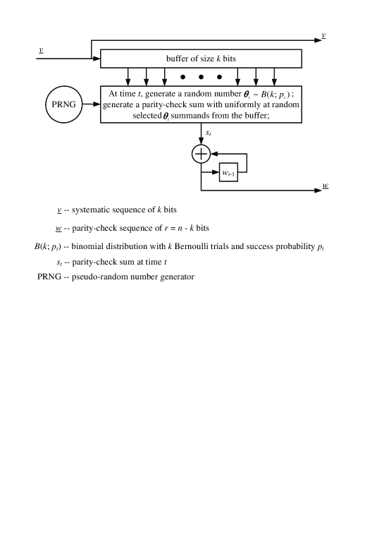
Figure 1: A systematic encoding algorithm for the proposed Kite code.

Algorithm 1

(Recursive encoding algorithm for Kite codes)

1. Initialization: Initially, set $w_{-1}=0$. Equivalently, set the initial state of the accumulator to be zero.

2. Recursion: For $t=0,1,\cdots,T-1$ with $T$ as large as required, compute $w_{t}$ recursively according to the following procedures.

   Step 2.1: At time $t\geq 0$, sampling from $k$ independent identically distributed (i.i.d.) binary random variables $\underline{H}_{t}=(H_{t,0},H_{t,1},\cdots,H_{t,k-1})$, where

   $${\rm Pr}\{H_{t,i}=h_{t,i}\}=\left\{\begin{array}[]{cc}p_{t},&h_{t,i}=1\\ 1-p_{t},&h_{t,i}=0\\ \end{array}\right.$$ (2)

   for $0\leq i<k$;

   Step 2.2: Compute the $t$-th parity-check bit by $w_{t}=w_{t-1}+\sum_{0\leq i<k}h_{t,i}v_{i}~{}{\rm mod}~{}2$.

Remark. Algorithm 1 can also be implemented by first sampling from the binomial distribution $B(k;p_{t})$ to obtain an integer $\theta_{t}$ and then choosing $\theta_{t}$ summands uniformly at random from the buffer to obtain a parity-check sum $s_{t}$, which is utilized to drive the accumulator, as shown in Fig. 1.

For convenience, the prefix code $\mathcal{K}[n,k]$ of a Kite code $\mathcal{K}[\infty,k;\underline{p}]$ is also called a Kite code. A Kite code $\mathcal{K}[n,k]$ for $n\geq k$ is a systematic linear code with $r\stackrel{{\scriptstyle\Delta}}{{=}}n-k$ parity-check bits. We can write its parity-check matrix $H$ as

$$H=\left(H_{v},H_{w}\right),$$ (3)

where $H_{v}$ is a matrix of size $r\times k$ that corresponds to the information bits, and $H_{w}$ is a square matrix of size $r\times r$ that corresponds to the parity-check bits. By construction, we can see that the sub-matrix $H_{v}$ is a random-like binary matrix whose entries are governed by the p-sequence and the initial state of the PRNG. In contrast, the square matrix $H_{w}$ is a dual-diagonal matrix (blanks represent zeros)

$$H_{w}=\left(\begin{array}[]{ccccc}1&&&&\\ 1&1&&&\\ &1&\ddots&&\\ &&\ddots&1&\\ &&&1&1\\ \end{array}\right).$$ (4)

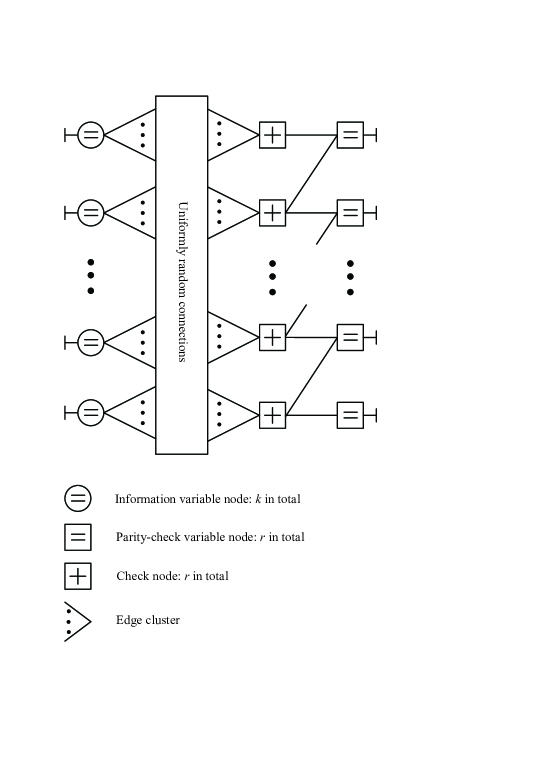
Figure 2: A normal graph of a Kite code.

Since the density of the parity-check matrix is dominated by the $p$-sequence, we can construct Kite codes as LDPC codes by choosing $p_{t}\ll 1/2$. If so, the receiver can perform the iterative sum-product decoding algorithm [4]. The iterative sum-product algorithm can be described as a message passing/processing algorithm on factor graphs [19]. A Forney-style factor graph (also called a normal graph [20]) representation of $\mathcal{K}[n,k]$ is shown in Fig. 2.

Now we assume that the coded bit $c_{t}$ at time $t\geq 0$ is modulated in a BPSK format and transmitted over the AWGN channel. With this assumption, an intended receiver observes a noisy version $y_{t}=x_{t}+z_{t}$, where $x_{t}=1-2c_{t}$ and $z_{t}$ is an AWGN sample at time $t$. The noise variance $\sigma^{2}$ is assumed to be known at the receiver. We also assume that the intended receiver has a large enough buffer to store the received sequence for the purpose of decoding.

Once a noisy prefix (of length $n$) ${\underline{y}}[n]$ is available, the receiver can perform the iterative sum-product decoding algorithm to get an estimate of the transmitted codeword ${\underline{c}}[n]$. The decoding is said to be successful if the decoder can find an estimate $\hat{\underline{c}}[n]$ within $J$ (a preset maximum iteration number) iterations satisfying all the parity-check equations specified by $H$. If not such a case, the receiver may collect more noisy bits to try the decoding again. If $n$ is the length of the prefix code that can be decoded successfully, we call $k/n$ decoding rate rather than coding rate. The decoding rate is a random variable, which may vary from frame to frame. However, the expectation of the decoding rate cannot exceed the corresponding channel capacity [21]. Given a signal-to-noise-ratio (SNR) of $1/\sigma^{2}$, the gap between the average decoding rate and the channel capacity can be utilized to evaluate the performance of the proposed Kite code. A rateless code is called universal if it is “good” in a wide range of SNRs. It is reasonable to guess that the universality of the proposed Kite code for given $k$ can be improved by properly choosing the $p$-sequence.

II-C Relations Between Kite Codes and Existing Codes

The proposed Kite codes are different from existing iteratively decodeable codes.

1. The Kite codes are different from general LDPC codes. An ensemble of Kite codes is systematic, rateless and characterized by the $p$-sequence, while an ensemble of general LDPC codes is usually non-systematic and characterized by two degree distributions $\lambda(x)=\sum_{i}\lambda_{i}x^{i-1}$ and $\rho(x)=\sum_{i}\rho_{i}x^{i-1}$, where $\lambda_{i}$ ($\rho_{i}$) represents the fraction of edges emanating from variable (check) nodes of degree $i$ [22][23].

2. The Kite codes can be considered as serially concatenated codes with systematic low-density generator-matrix (LDGM) codes [24] as outer codes and an accumulator as inner code. However, different from conventional serially concatenated codes, the inner code takes only the parity-check bits from the outer codes as input bits. An another difference is as follows. The generator matrices $H_{v}^{\bf T}$ (transpose of $H_{v}$) of outer LDGM codes may have infinite columns with random weights governed by the $p$-sequence rather than degree polynomials.

3. The Kite codes are also similar to the generalized irregular repeat-accumulate (GeIRA) codes [25][26][27][28]. However, GeIRA codes are usually specified by the repetition multiplicities of each information bits and the uniform interleaver.

4. As a rateless coding method, the proposed Kite codes are different from LT-codes and Raptor codes. For LT-codes and Raptor codes, coded bits are generated independently according to a time-independent degree distribution; while for Kite codes, parity-check bits are generated dependently. The Kite codes are more similar to the codes proposed in [29], which are designed for erasure channels and specified by degree polynomials.

As an ensemble of codes, the proposed Kite codes are new. The main feature of Kite codes is the use of the $p$-sequence instead of degree distributions to define the ensemble. This has brought at least two advantages. Firstly, as shown in Sec. III, the weight enumerating function (WEF) of the ensemble can be easily calculated, implying that the ML decoding performance of Kite codes can be analyzed. Secondly, as shown in Sec. IV, Kite codes can be designed by a greedy optimization algorithm which consists of several one-dimensional search rather than high-dimensional differential evolution algorithms [30] [31].

III Maximum Likelihood Decoding Analysis of Kite Codes

III-A Weight Enumerating Function of the Ensemble of Kite Codes

We can define the input-redundancy weight enumerating function (IRWEF) of an ensemble of (prefix) Kite codes with dimension $k$ and length $n$ as [32]

$$A(X,Z)\stackrel{{\scriptstyle\Delta}}{{=}}\sum\limits_{i,j}A_{i,j}X^{i}Z^{j},$$ (5)

where $X,Z$ are two dummy variables and $A_{i,j}$ denotes the ensemble average of the number of codewords $\underline{c}=(\underline{v},\underline{w})$ consisting of an input information sequence $\underline{v}$ of Hamming weight $i$ and a parity check sequence $\underline{w}$ of Hamming weight $j$.

Let $\underline{v}^{(\ell)}$ be an input sequence consisting of $\ell$ ones followed by $k-\ell$ zeros. That is, $\underline{v}^{(\ell)}\stackrel{{\scriptstyle\Delta}}{{=}}(\underbrace{1\cdots 1}_{\ell}\underbrace{0\cdots 0}_{k-\ell})$. Let $\underline{w}^{(\ell)}$ be the resulting parity-check sequence, which is a sample of a random sequence $\underline{W}^{(\ell)}$ depending on the choice of the parity-check matrix. Given $\underline{v}^{(\ell)}$, the probability ${\rm Pr}\{W_{t}^{(\ell)}=1\}$ can be determined recursively as follows.

Firstly, note that the random binary sum (see Fig. 1 for the notation $s_{t}$) $S_{t}^{(\ell)}=\sum\limits_{0\leq i\leq\ell-1}H_{t,i}$. So $p_{t}^{(\ell)}\stackrel{{\scriptstyle\Delta}}{{=}}{\rm Pr}\{S_{t}^{(\ell)}=1\}$ can be calculated recursively as $p_{t}^{(\ell)}=p_{t}^{(\ell-1)}(1-p_{t})+(1-p_{t}^{(\ell-1)})p_{t}$ for $\ell>0$ whereby $p_{t}^{(0)}$ is initialized as zero. Secondly, we note that the sequence $\underline{W}^{(\ell)}$ is a Markov process with the following time-dependent transition probabilities

$$\begin{array}[]{ll}{\rm Pr}\{W_{t}^{(\ell)}=0\mid W_{t-1}^{(\ell)}=0\}=1-p_{t}^{(\ell)},&{\rm Pr}\{W_{t}^{(\ell)}=1\mid W_{t-1}^{(\ell)}=0\}=p_{t}^{(\ell)},\\ {\rm Pr}\{W_{t}^{(\ell)}=0\mid W_{t-1}^{(\ell)}=1\}=p_{t}^{(\ell)},&{\rm Pr}\{W_{t}^{(\ell)}=1\mid W_{t-1}^{(\ell)}=1\}=1-p_{t}^{(\ell)}.\\ \end{array}$$ (6)

We have the following two propositions.

Proposition 1

Let $A^{(\ell)}(Z)$ be the ensemble average weight enumerating function of $\underline{W}^{(\ell)}$. Let $\alpha_{t}(Z;w)$ be the ensemble average weight enumerating function of the prefix sequence $\underline{W}^{(\ell,t)}=(W^{(\ell)}_{0},W^{(\ell)}_{1},\cdots,W^{(\ell)}_{t})$ ending with $W^{(\ell)}_{t}=w$ at time $t$. Then $A^{(\ell)}(Z)$ can be calculated recursively by performing a forward trellis-based algorithm (see Fig. 3 for the trellis representation) over the polynomial ring.

• Initially, set $\alpha_{-1}(Z;0)=1$ and $\alpha_{-1}(Z;1)=0$;

• For $t\geq 0$,

  $$\alpha_{t}(Z;0) = (1-p_{t}^{(\ell)})\alpha_{t-1}(Z;0)+p_{t}^{(\ell)}\alpha_{t-1}(Z;1)$$

  $$\alpha_{t}(Z;1) = p_{t}^{(\ell)}Z\cdot\alpha_{t-1}(Z;0)+(1-p_{t}^{(\ell)})Z\cdot\alpha_{t-1}(Z;1)$$

• At time $r-1$, we have $A^{(\ell)}(Z)=\alpha_{r-1}(Z;0)+\alpha_{r-1}(Z;1)$.

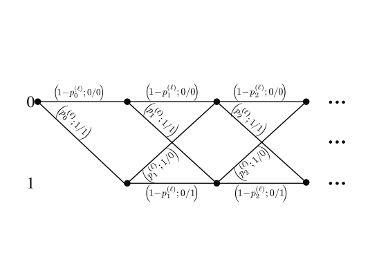
Figure 3: The trellis representation of the random parity-check sequence $\underline{W}^{(\ell)}$. To calculate the ensemble WEF, we assign to each branch a metric ${\rm Pr}\{S_{t}^{(\ell)}=s_{t}\}\cdot Z^{w_{t}}$, where $s_{t}/w_{t}$ are the input/output associated with the branch, respectively.

Proof:

The algorithm is similar to the trellis algorithm over polynomial rings for computing the weight enumerators of paths [33]. The difference is that each path here has a probability, which can be incorporated into the recursions by assigning to each branch the corresponding transition probability as a factor of the branch metric. ∎

Proposition 2

$A(X,Z)=\sum\limits_{0\leq\ell\leq k}\left(\begin{array}[]{c}k\\ \ell\\ \end{array}\right)X^{\ell}A^{(\ell)}(Z)$.

Proof:

By the construction, we can see that the columns of $H_{v}$ are identically independent distributed. This implies that $A^{(\ell)}(Z)$ depends only on the Hamming weight $\ell$ of $\underline{v}$ but not on the locations of the $\ell$ ones in the sequence $\underline{v}$. ∎

III-B Refined Divsalar Bound

We now proceed to discuss the ML decoding performance of Kite codes. Consider the prefix code $\mathcal{K}[n,k;\underline{p}]$. Assume that the all-zero codeword $\underline{c}^{0}[n]$ is transmitted and $\underline{y}[n]$ is the received vector with $y_{t}=1-2c_{t}+z_{t}$ and $z_{t}$ is an AWGN sample with zero mean and variance $\sigma^{2}$. The probability of ML decoding error can be expressed as

$${\rm Pr}\left\{E\right\}={\rm Pr}\left\{\bigcup_{d}E_{d}\right\},$$ (7)

where $E_{d}$ is the event that there exists at least one codeword of weight $d$ that is nearer to $\underline{y}[n]$ than $\underline{c}^{0}[n]$.

Let $S_{d}=\sum\limits_{i,j:i+j=d}A_{i,j}$ for all $0\leq d\leq n$. Divsalar derived a simple upper bound [34][35]

$${\rm Pr}\{E_{d}\}\leq\min\left\{e^{-nE(\delta,\beta,\gamma)},S_{d}Q\left(\sqrt{2d\gamma}\right)\right\},$$ (8)

where

$$E(\delta,\beta,\gamma)=-r_{n}(\delta)+\frac{1}{2}\ln\left(\beta+(1-\beta)e^{2r_{n}(\delta)}\right)+\frac{\beta\gamma\delta}{1-(1-\beta)\delta}$$ (9)

and $\gamma=\frac{E_{s}}{2\sigma^{2}}$, $\delta=d/n$, $r_{n}(\delta)=\frac{\ln S_{d}}{n}$ and

$$\beta=\sqrt{\frac{\gamma(1-\delta)}{\delta}\frac{2}{1-e^{-2r_{n}(\delta)}}+\left(\frac{1-\delta}{\delta}\right)^{2}\left[(1+\gamma)^{2}-1\right]}-\frac{1-\delta}{\delta}(1+\gamma).$$ (10)

From (8) and the union bound, we have

$${\rm Pr}\left\{E\right\}\leq\sum_{d}\min\left\{e^{-nE(\delta,\beta,\gamma)},S_{d}Q\left(\sqrt{2d\gamma}\right)\right\}.$$ (11)

The question is, how many terms do we need to count in the above bound? If too few terms are counted, we will obtain a lower bound of the upper bound, which may be neither an upper bound nor a lower bound; if too many are counted, we need pay more effort to compute the distance distribution and we will obtain a loose upper bound. To get a tight upper bound, we may determine the terms by analyzing the facets of the Voronoi region of the codeword $\underline{c}^{0}[n]$, which is a difficult task for a general code. We have proposed a technique to reduce the number of terms [36]. For completeness, we include a brief description of the technique here. The basic idea is to limit the competitive candidate codewords by using the following suboptimal algorithm.

Algorithm 2

(A list decoding algorithm for the purpose of performance analysis)

1. Make hard decisions, for $0\leq t\leq n-1$,

   $$\hat{y}_{t}=\left\{\begin{array}[]{cc}0,&y_{t}>0\\ 1,&y_{t}\leq 0\end{array}\right..$$ (12)

   Then the channel $c_{t}\rightarrow\hat{y}_{t}$ becomes a memoryless binary symmetric channel (BSC) with cross probability

   $$p_{BSC}=Q\left(\frac{1}{\sigma}\right)\stackrel{{\scriptstyle\Delta}}{{=}}\int_{1/\sigma}^{+\infty}\frac{1}{\sqrt{2\pi}}e^{-\frac{z^{2}}{2}}\,{\rm d}z.$$ (13)

2. List all codewords within the Hamming sphere with center at $\underline{\hat{y}}$ of radius $d^{*}\geq 0$. The resulted list is denoted as $\mathcal{L}_{\underline{y}}$.

3. If $\mathcal{L}_{\underline{y}}$ is empty, report a decoding error; otherwise, find the codeword $\underline{c}^{*}\in\mathcal{L}_{\underline{y}}$ that is closest to $\underline{y}[n]$.

Now we define

$$\mathcal{R}\stackrel{{\scriptstyle\Delta}}{{=}}\left\{\underline{y}|{\underline{c}}^{0}[n]\in\mathcal{L}_{\underline{y}}\right\}.$$ (14)

In words, the region $\mathcal{R}$ consists of all those $\underline{y}[n]$ having at most $d^{*}$ non-positive components. The decoding error occurs in two cases under the assumption that the all-zero codeword ${\underline{c}}^{0}[n]$ is transmitted.

Case 1. The all-zero codeword is not in the list $\mathcal{L}_{\underline{y}}$ (see Fig. 4 (a)), that is, $\underline{y}[n]\notin\mathcal{R}$, which means that at least $d^{*}+1$ errors occur over the BSC. This probability is

$${\rm Pr}\left\{\underline{y}[n]\notin\mathcal{R}\right\}=\sum_{t=d^{*}+1}^{n}\binom{n}{t}p_{BSC}^{t}(1-p_{BSC})^{n-t}.$$ (15)

Case 2. The all-zero codeword is in the list $\mathcal{L}_{\underline{y}}$, but is not the closest one (see Fig. 4 (b)), which is equivalent to the event $\left\{E,\underline{y}[n]\in\mathcal{R}\right\}$. Since all codewords in the list $\mathcal{L}_{\underline{y}}$ are at most $2d^{*}$ away from the all-zero codeword, this probability is upper-bounded by

$${\rm Pr}\left\{E,\underline{y}[n]\in\mathcal{R}\right\} \leq {\rm Pr}\left\{\bigcup_{d\leq 2d^{*}}E_{d},\;\;\underline{y}[n]\in\mathcal{R}\right\}$$ (16)

$$\leq {\rm Pr}\left\{\bigcup_{d\leq 2d^{*}}E_{d},\;\;\underline{y}[n]\in\mathbb{R}^{n}\right\}$$ (17)

$$\leq \sum_{d\leq 2d^{*}}{\rm Pr}\left\{E_{d}\right\}$$ (18)

$$\leq \sum_{d\leq 2d^{*}}\min\left\{e^{-nE(\delta,\beta,\gamma)},S_{d}Q\left(\sqrt{2d\gamma}\right)\right\}.$$ (19)

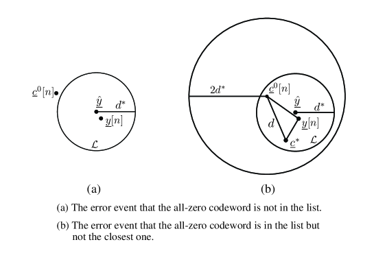
Figure 4: Graphical illustrations of the decoding error events.

Combining (15) and (19) with Gallager’s first bounding technique (GFBT) [37]

$${\rm Pr}\{E\}\leq{\rm Pr}\{E,{\underline{y}}[n]\in\mathcal{R}\}+{\rm Pr}\{{\underline{y}}[n]\notin\mathcal{R}\},$$ (20)

we get an upper bound

$${\rm Pr}\{E\}\leq\sum_{d\leq 2d^{*}}\min\left\{e^{-nE(\delta,\beta,\gamma)},S_{d}Q\left(\sqrt{2d\gamma}\right)\right\}+\sum_{t>d^{*}}\binom{n}{t}p_{BSC}^{t}(1-p_{BSC})^{n-t}.$$ (21)

To calculate the upper bound on bit-error probability, we need to replace $S_{d}$ in (21) by

$$S^{\prime}_{d}=\sum\limits_{i,j:i+j=d}\frac{i}{k}A_{i,j}.$$ (22)

Here we have used the fact that, in the case of ${\underline{c}}^{0}[n]\notin\mathcal{L}_{\underline{y}}$, the decoding error can contribute at most one to the bit-error rate (BER).

The modified upper bound in (21) has advantageous over the original Divsalar bound (11). On one hand, the modified upper bound in (21) is less complex than the original Divsalar bound (11) for codes having no closed-form WEFs since its computation only involves portion of the weight spectrum up to $d\leq 2d^{*}$. On the other hand, if all $A_{i,j}$’s for $i+j\leq D$ are available, we can get a tighter upper bound

$${\rm Pr}\{E\}\leq\min_{d^{*}\leq D/2}\left\{\sum_{d\leq 2d^{*}}\min\left\{e^{-nE(\delta,\beta,\gamma)},S_{d}Q\left(\sqrt{2d\gamma}\right)\right\}+\sum_{t>d^{*}}\binom{n}{t}p_{BSC}^{t}(1-p_{BSC})^{n-t}\right\},$$ (23)

which can be tighter than the original Divsalar bound (11) (corresponding to $d^{*}=n$).

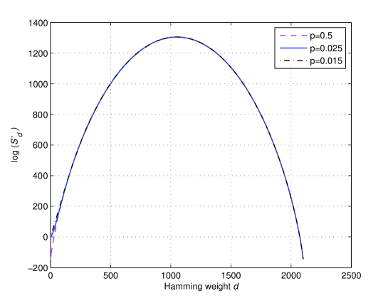
Figure 5: Ensemble weight enumerating functions of $\mathcal{K}[2100,1890]$.

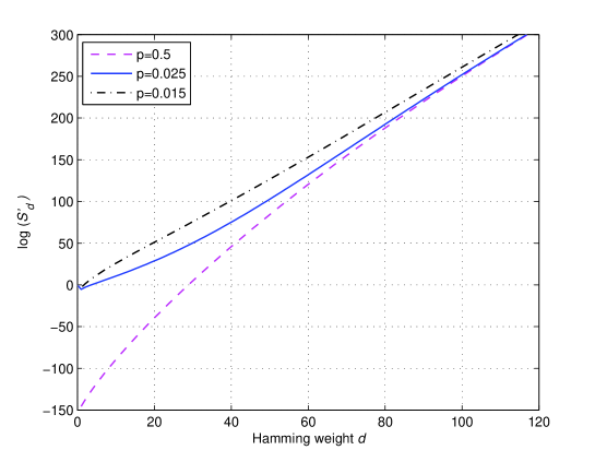
Figure 6: Detailed ensemble weight enumerating functions of $\mathcal{K}[2100,1890]$.

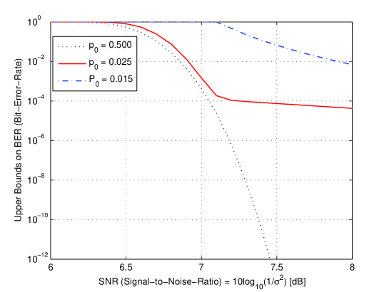
Figure 7: Performance bounds on the ensemble Kite codes $\mathcal{K}[2100,1890]$.

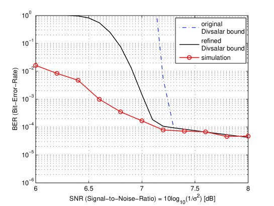
Figure 8: Comparisons between bounds and simulation results for $p=0.025$.

III-C Numerical Results

We consider a Kite code $\mathcal{K}[2100,1890]$. For simplicity, set $p_{t}=p_{0}$ for all $t<210$. We consider $p_{0}=0.5,0.025$ and $0.015$, respectively. The WEFs $\{S^{\prime}_{d}\}$ are shown in Fig. 5. As we can see, the three curves match well in the moderate-to-high-weight region. While, in the low-weight region, they differs much from each other, as shown in Fig. 6. As the parameter $p_{0}$ increases to $0.5$, the resulting ensemble becomes a uniformly random ensemble. The refined Divsalar bounds on BERs are shown in Fig. 7. Shown in Fig. 8 are the comparisons between bounds and simulation results for $p_{0}=0.025$. We have the following observations.

1. The modified bound improves the original Divsalar bound especially in the low-SNR region.

2. Under the assumption of the ML decoding, the performance degrades as the parameter $p_{0}$ decreases. There exists an error floor at BER around $10^{-4}$ for $p_{0}=0.025$. At the corner of the floor, the performance gap (in terms of upper bounds) between the code with $p_{0}=0.025$ and the totally random code is less than $0.1$ dB.

3. The iterative sum-product decoding algorithm delivers a curve that matches well with the performance bounds of the ML decoding in the high-SNR region.

IV Design of Kite Codes

IV-A Partition the $p$-Sequence According to Decoding Rates

As we have observed in Section III that the choices of the $p$-sequence have effect on the performance of Kite codes. On one hand, to ensure with high probability that the resulting Kite codes are iteratively decodable LDPC codes, we must choose the $p$-sequence such that $p_{t}\ll 1/2$. On the other hand, to guarantee the performance, the components of the $p$-sequence can not be too small.

The task to optimize a Kite code is to select the whole $p$-sequence such that all the prefix codes are good enough. This is a multi-objective optimization problem and could be very complex. For simplicity, we only consider the codes with rates not less than 0.1 and simply group the $p$-sequence according to decoding rates as follows

$$p_{t}=\left\{\begin{array}[]{rl}q_{9},&0.9\leq k/(t+k)<1.0\\ q_{8},&0.8\leq k/(t+k)<0.9\\ q_{7},&0.7\leq k/(t+k)<0.8\\ q_{6},&0.6\leq k/(t+k)<0.7\\ q_{5},&0.5\leq k/(t+k)<0.6\\ q_{4},&0.4\leq k/(t+k)<0.5\\ q_{3},&0.3\leq k/(t+k)<0.4\\ q_{2},&0.2\leq k/(t+k)<0.3\\ q_{1},&0.1\leq k/(t+k)<0.2\\ \end{array}\right..$$ (24)

Then the task to design a Kite code is to select the parameters $\underline{q}=(q_{9},q_{8},\cdots,q_{1})$.

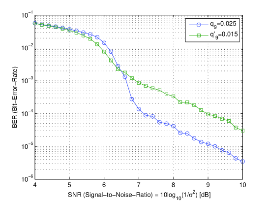
Figure 9: BER performance of $\mathcal{K}[2100,1890]$.

IV-B Greedy Optimizing Algorithms

We use a greedy algorithm to optimize the parameters $\underline{q}$. Firstly, we choose $q_{9}$ such that the prefix code $\mathcal{K}[\lfloor k/0.9\rfloor,k]$ is as good as possible. Secondly, we choose $q_{8}$ with fixed $q_{9}$ such that the prefix code $\mathcal{K}[\lfloor k/0.8\rfloor,k]$ is as good as possible. Thirdly, we choose $q_{7}$ with fixed $(q_{9},q_{8})$ such that the prefix code $\mathcal{K}[\lfloor k/0.7\rfloor,k]$ is as good as possible. This process continues until $q_{1}$ is selected.

Let $q_{\ell}$ be the parameter to be optimized. Since the parameters $q_{j}$ with $j>\ell$ have been fixed and the parameters $q_{j}$ with $j<\ell$ are irrelevant to the current prefix code, the problem to design the current prefix code then becomes a one-dimensional optimization problem, which can be solved, for example, by the golden search method [38]. What we need to do is to make a choice between any two candidate parameters $q_{\ell}$ and $q^{\prime}_{\ell}$, which can be done (with certain BER performance criterion) by at least two methods. We take $k=1890$ as an example to illustrate the main idea.

IV-B1 Simulation-Based Methods

We can first simulate the BER versus SNR curves and then make a choice between $q_{\ell}$ and $q^{\prime}_{\ell}$. For example, Fig. 9 illustrates our simulations for $\mathcal{K}[2100,1890]$. If the target is $\textrm{BER}<10^{-3}$, we say that $q_{9}=0.025$ is superior to $q^{\prime}_{9}=0.015$. At first glance, such a simulation-based method could be very time-consuming. However, it is fast due to the following two reasons. Firstly, in this paper, our optimization target is set to be $\textrm{BER}=10^{-4}$, which can be reliably estimated without large amounts of simulations. Secondly, our goal is not to reliably estimate the performances corresponding to the two parameters $q_{\ell}$ and $q^{\prime}_{\ell}$ but to make a choice between these two parameters. Making a choice between two design parameters, as an example of ordinal optimization problem [39], can be easily done by simulations.

IV-B2 Density Evolution

We can also make a choice between $q_{\ell}$ and $q^{\prime}_{\ell}$ by using density evolution. As shown in Fig. 2, the Kite code can be represented by a normal graph which contains three types of nodes: information variable nodes, parity-check variable nodes and check nodes, which are simply referred to as $A$-type nodes, $B$-type nodes and $C$-type nodes, respectively. Since the connections between $B$-type nodes and $C$-type nodes are deterministic, we only need to derive the degree distributions for the edges between $A$-nodes and $C$-nodes.

Node degree distributions: Assume that the parameters $q_{j}$ for $j>\ell$ have been optimized and fixed. The resulting parity-check matrix is written as $H^{(\ell+1)}=(H_{v}^{(\ell+1)},H_{w}^{(\ell+1)})$, which is a random matrix of size $r^{(\ell+1)}\times(k+r^{(\ell+1)})$. In our settings, for example, $r^{(9)}=\lfloor k/0.9\rfloor-k$, $r^{(8)}=\lfloor k/0.8\rfloor-k$, and so on. Noting that $H^{(\ell)}$ is constructed from $H^{(\ell+1)}$ by adding $\delta=r^{(\ell)}-r^{(\ell+1)}$ rows, we may write it as

$$H^{(\ell)}=(H_{v}^{(\ell)},H_{w}^{(\ell)})=\left(\begin{array}[]{cc}H_{v}^{(\ell+1)}&H_{w}^{(\ell+1)}\\ H_{v}^{(\delta)}&H_{w}^{(\delta)}\\ \end{array}\right).$$ (25)

Since $H_{w}^{(\ell)}$ is deterministic, we only need to determine the degree distributions of nodes corresponding to $H_{v}^{(\ell)}$. For doing so, assume that the degree distributions of nodes corresponding to $H_{v}^{(\ell+1)}$ are, for $A$-type nodes,

$$\Lambda^{(\ell+1)}(x)=\sum_{0\leq i\leq r^{(\ell+1)}}\Lambda_{i}^{(\ell+1)}x^{i},$$ (26)

and for $C$-type nodes,

$$R^{(\ell+1)}(x)=\sum_{0\leq i\leq k}R_{i}^{(\ell+1)}x^{i},$$ (27)

where $\Lambda_{i}^{(\ell+1)}$ (resp. $R_{i}^{(\ell+1)}$) represents the fraction of $A$-type (resp. $C$-type) nodes of degree $i$. In our settings, for example, $\Lambda_{i}^{(9)}=\binom{r^{(9)}}{i}q_{9}^{i}(1-q_{9})^{r^{(9)}-i}$ for $0\leq i\leq r^{(9)}$ and $R_{i}^{(9)}=\binom{k}{i}q_{9}^{i}(1-q_{9})^{k-i}$ for $0\leq i\leq k$. Since $\Lambda_{0}^{(9)}>0$, there may exist nodes with no edges. However, such a probability can be very small for large $r^{(9)}$. It should also be pointed out that $R^{(\ell+1)}(x)$ only counts the edges of the $C$-type nodes connecting to the $A$-type nodes. For this reason, we call $R^{(\ell)}(x)$ the left degree distribution of $C$-nodes.

Let $\Lambda(x)=\sum_{0\leq i\leq\delta}\Lambda_{i}x^{i}$ and $R(x)=\sum_{0\leq i\leq k}R_{i}x^{i}$ be the degree distributions of nodes corresponding to $H_{v}^{(\delta)}$. Then we have

$$\Lambda_{i}=\binom{\delta}{i}q_{\ell}^{i}(1-q_{\ell})^{\delta-i},\;\;0\leq i\leq\delta$$ (28)

and

$$R_{i}=\binom{k}{i}q_{\ell}^{i}(1-q_{\ell})^{k-i},\;\;0\leq i\leq k.$$ (29)

Then it is not difficult to verify that

$$\Lambda_{i}^{(\ell)}=\sum_{i=j+k}\Lambda_{j}\Lambda_{k}^{(\ell+1)},\;\;0\leq i\leq r^{(\ell)}$$ (30)

and

$$R_{i}^{(\ell)}=\frac{r^{(\ell+1)}R^{(\ell)}_{i}+\delta R_{i}}{r^{(\ell)}},\;\;0\leq i\leq k.$$ (31)

Edge degree distributions: Given $\Lambda^{(\ell)}(x)$ and $R^{(\ell)}(x)$ (which can be computed recursively), we can find the degree distributions of edges between $A$-type nodes and $C$-type nodes as follows. Let $\lambda(x)=\sum_{i}\lambda_{i}x^{i-1}$ and $\rho(x)=\sum_{i}\rho_{i}x^{i-1}$ be the degree distributions of edges corresponding to $H_{v}^{(\ell)}$. We have

$$\lambda_{i}=\frac{i\Lambda_{i}}{\sum_{j}j\Lambda_{j}},\;\;1\leq i\leq r^{(\ell)}$$ (32)

and

$$\rho_{i}=\frac{iR_{i}}{\sum_{j}jR_{j}},\;\;1\leq i\leq k.$$ (33)

Gaussian Approximation: The density evolution [23] is an algorithm that predicts the performance thresholds of random LDPC codes by tracing the probability density function (pdf) of the messages exchanging between different types of nodes under certain assumptions. In the density evolution, we assume that the all-zero codeword is transmitted. It is convenient to assume that the input messages to the decoder are initialized by the following log-likelihood ratios (LLRs)

$$M_{0}=\log\frac{f_{Y}(y|+1)}{f_{Y}(y|-1)},$$ (34)

where $f_{Y}$ is the conditional pdf of $Y$ given that $+1$ is transmitted. It has been proven [23] that, for the BPSK input and continuous output AWGN channel, $M_{0}$ is a Gaussian random variable having mean $\mu_{0}=2/\sigma^{2}$ and satisfying the symmetry condition $\sigma_{0}^{2}=2\mu_{0}$. It was further shown [40] that all the intermediate messages produced during the iterative sum-product algorithm can be approximated by Gaussian variables or mixture of Gaussian variables satisfying the symmetry condition. This means that we need to trace only the means of the messages.

For Kite codes shown in Fig. 2, the density evolution using Gaussian approximations are slightly different from that general LDPC codes. To describe the algorithm more clearly, we introduce the following notation.

$~{}~{}~{}\mu_{0}$   the mean of initial messages from the channel;
$\mu_{i}^{(A\rightarrow C)}$   the mean of messages from $A$-type nodes of degree $i$ to $C$-type nodes;
$\mu^{(B\rightarrow C)}$   the mean of messages from $B$-type nodes to $C$-type nodes;
$\mu_{i}^{(C\rightarrow A)}$   the mean of messages from $C$-type nodes of left degree $i$ to $A$-type nodes;
$\overline{\mu}^{(C\rightarrow A)}$   the average mean of messages from $A$-type nodes to $C$-type nodes;
$\mu_{i}^{(C\rightarrow B)}$   the mean of messages from $C$-type nodes of left degree $i$ to $B$-type nodes;
$\overline{\mu}^{(C\rightarrow B)}$   the average mean of messages from $C$-type nodes to $B$-type nodes.

Slightly different from [40] but following [41], we define

$$\phi(x)\stackrel{{\scriptstyle\Delta}}{{=}}\left\{\begin{array}[]{ll}\frac{1}{\sqrt{4\pi x}}\int^{+\infty}_{-\infty}\tanh(y/2)e^{-(y-x)^{2}/(4x)}dy,&x>0\\ 0,&x=0\end{array}\right..$$ (35)

We may use the following algorithm to predict the performance threshold for the considered parameter $q_{\ell}$ under the iterative sum-product decoding algorithm.

Algorithm 3

(Density evolution using Gaussian approximations for Kite codes)

1. Input: The degree distributions of nodes $\Lambda(x)$, $R(x)$; the degree distributions of edges $\lambda(x)$, $\rho(x)$; target $T_{b}$ of BER and absolute difference $\Delta_{b}$ of BERs for two successive iterations;

2. Initializations: Set $\varepsilon=\int^{0}_{-\infty}\frac{1}{\sqrt{4\pi\mu_{0}}}e^{-(y-\mu_{0})^{2}/(4\mu_{0})}dy$, $\overline{\mu}^{(C\rightarrow A)}=0$ and $\overline{\mu}^{(C\rightarrow B)}=0$;

3. iterations - Repeat:

   Step 3.1: From $A$-type nodes to $C$-type nodes,

   $$\mu^{(A\rightarrow C)}_{i}=\mu_{0}+(i-1)\overline{\mu}^{(C\rightarrow A)},1\leq i\leq r;$$ (36)

   Step 3.2: From $B$-type nodes to $C$-type nodes,

   $$\mu^{(B\rightarrow C)}=\mu_{0}+\overline{\mu}^{(C\rightarrow B)};$$ (37)

   Step 3.3:

   1. From $C$-type nodes to $A$-type nodes,

      $$\mu^{(C\rightarrow A)}_{j}=\phi^{-1}\left(\phi^{2}(\mu^{(B\rightarrow C)})\left(\sum_{i=1}^{r}\lambda_{i}\phi(\mu_{i}^{(A\rightarrow C)})\right)^{j-1}\right),1\leq j\leq k;$$ (38)

      $$\overline{\mu}^{(C\rightarrow A)}=\sum\limits_{j=1}^{k}\rho_{j}\mu^{(C\rightarrow A)}_{j};$$ (39)

   2. From $C$-type nodes to $B$-type nodes,

      $$\mu^{(C\rightarrow B)}_{j}=\phi^{-1}\left(\phi(\mu^{(B\rightarrow C)})\left(\sum_{i=1}^{r}\lambda_{i}\phi(\mu_{i}^{(A\rightarrow C)})\right)^{j}\right),0\leq j\leq k;$$ (40)

      $$\overline{\mu}^{(C\rightarrow B)}=\sum\limits_{j=0}^{k}R_{j}\mu^{(C\rightarrow B)}_{j};$$ (41)

   Step 3.4: Make decisions, for $0\leq i\leq r$, define $\mu_{i}\stackrel{{\scriptstyle\Delta}}{{=}}\mu_{0}+i\overline{\mu}^{(C\rightarrow A)}$; compute

   $$\varepsilon_{i}=\int^{0}_{-\infty}\frac{1}{\sqrt{4\pi\mu_{i}}}e^{-(y-\mu_{i})^{2}/(4\mu_{i})}dy$$ (42)

   and

   $$\varepsilon^{\prime}=\sum\limits_{i=0}^{r}\Lambda_{i}\varepsilon_{i};$$ (43)

   if $\varepsilon^{\prime}\leq T_{b}$ or $|\varepsilon-\varepsilon^{\prime}|\leq\Delta_{b}$, exit the iteration; else set $\varepsilon=\varepsilon^{\prime}$ and go to Step 3.1.

Remark. Note that we have ignored the effect caused by the margin of the subgraph consisting of $B$-type nodes and $C$-type nodes. Also note that, different from the density evolution for general LDPC codes, degree distributions of nodes are also involved here.

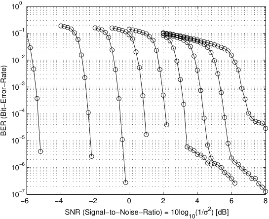
Figure 10: Performance of the constructed Kite code with $k=1890$. From left to right, the curves correspond to rates 0.1, 0.2, 0.3, 0.4, 0.5, 0.6, 0.7, 0.8, and 0.9, respectively.

IV-C Construction Examples

In this subsection, we present a construction example. We take the data length $k=1890$. A Kite code $\mathcal{K}[\infty,1890;\underline{p}]$ can be constructed using the following $p$-sequence

$$p_{t}=\left\{\begin{array}[]{rl}q_{9}=0.0249,&0.9\leq k/(t+k)<1.0\\ q_{8}=0.0072,&0.8\leq k/(t+k)<0.9\\ q_{7}=0.0045,&0.7\leq k/(t+k)<0.8\\ q_{6}=0.0034,&0.6\leq k/(t+k)<0.7\\ q_{5}=0.0021,&0.5\leq k/(t+k)<0.6\\ q_{4}=0.0016,&0.4\leq k/(t+k)<0.5\\ q_{3}=0.0010,&0.3\leq k/(t+k)<0.4\\ q_{2}=0.0006,&0.2\leq k/(t+k)<0.3\\ q_{1}=0.0004,&0.1\leq k/(t+k)<0.2\\ \end{array}\right..$$ (44)

The simulation results are shown in Fig. 10. For comparison, the SNR for the simulation at $\textrm{BER}=10^{-4}$ and the SNR thresholds estimated by the Gaussian-approximation-based density evolution (GA DE) are listed in the Table I. As we can see, the difference between the density evolution and the simulation is less than 1 dB.

TABLE I: The SNR for the density evolution and simulation at $\textrm{BER}=10^{-4}$.

Code rate	GA DE (dB)	Simulation (dB)
0.9	6.49	7.0
0.8	4.84	5.6
0.7	3.65	4.4
0.6	2.57	3.2
0.5	1.48	2.1
0.4	0.31	0.9
0.3	-1.04	-0.5
0.2	-2.84	-2.4
0.1	-5.67	-5.3

V Serial Concatenation of Reed-Solomon Codes and Kite Codes

V-A Encoding

Naturally, the proposed encoding method can be utilized to construct fixed-rate codes. However, we found by simulation that, in the range of moderate-to-high rates, the constructed fixed-rate codes in this way suffer from error-floors at BER around $10^{-4}$, as shown in Fig. 10. The error floor is caused by the possibly existing the all-zero columns in the randomly generated parity-check matrices. To lower-down the error-floor, we may insert some fixed-patterns into the matrices, as proposed in [42]. We also note that, in the rateless coding scenario, the receiver must find a way to ensure the correctness of the successfully decoded codeword. This is trivial for erasure channels but becomes complex for noisy channels. For erasure channels, a decoded codeword is correct if and only if all information bits are recovered uniquely. For AWGN channels, no simple way to ensure with probability one the correctness of the decoded codeword at the receiver. In order to lower down the error-floors and ensure with high probability the correctness of the decoded codewords, we employ the serially concatenated coding system proposed by Forney [1]. As shown in Fig. 11, the outer code is a systematic RS code of dimension $K$ and length $N$ over $\mathbb{F}_{2^{m}}$, while the inner code is a Kite code. Note that no interleaver is required between the outer encoder and the inner encoder. For convenience, such a concatenated code is called an RS-Kite code.

Let $\underline{u}$ be the binary data sequence of length $\ell mK$ ($\ell>0$). The encoding procedure is described as follows. First, the binary sequence $\underline{u}$ is interpreted as a $2^{m}$-ary sequence of length $\ell K$ and encoded by the outer encoder, producing $\ell$ RS codewords. Then these $\ell$ RS codewords are interpreted as a binary sequence $\underline{v}$ of length $\ell mN$ and encoded using a Kite code, resulting in a potentially infinite coded sequence $\underline{c}$.

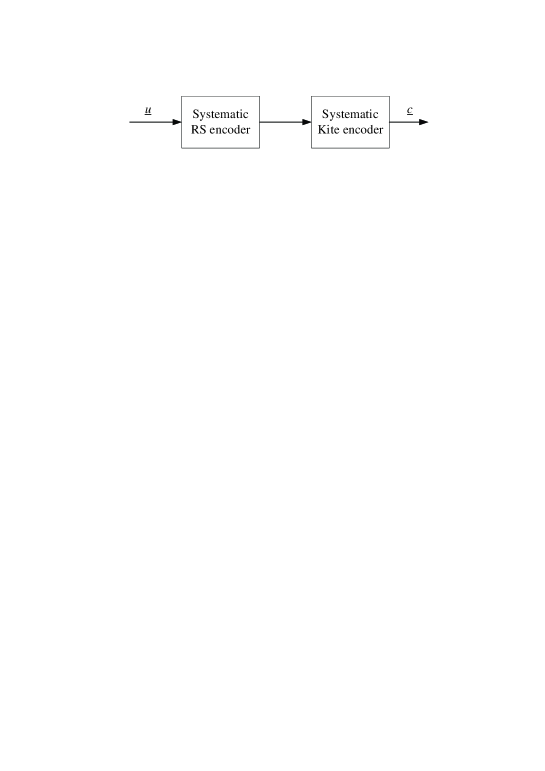
Figure 11: Serial concatenation of RS codes and Kite Codes.

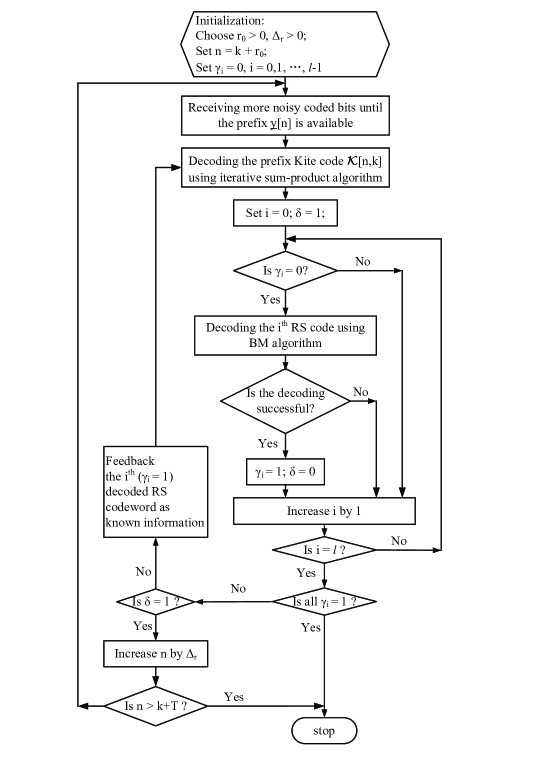
Figure 12: A flowchart of the decoding algorithm for the proposed serially concatenated codes.

V-B Decoding

We will use Berlekamp-Massey (BM) algorithm [43] for the outer decoder and iterative sum-product algorithm for the inner decoder. As we know, if the number of errors in a noisy RS codeword is not greater than $t_{max}\stackrel{{\scriptstyle\Delta}}{{=}}\lfloor(N-K)/2\rfloor$, the BM algorithm will find the correct codeword. On the other hand, if the number of errors in a noisy RS codeword is greater than $t_{max}$, the BM algorithm may claim a decoding failure or make a miscorrection. We call the BM decoding successful whenever the BM algorithm finds a codeword within the Hamming sphere of radius $t_{max}$ around the received “codeword” from the inner decoder. Since the miscorrection probability can be made very small by properly setting the parameters of the RS code [44][45], we will treat the successfully decoded RS codewords as “side information” (prior known information) for the inner decoder. For $\ell>1$, such known information can be fed back to the inner decoder to implement iterations between the outer decoder and the inner decoder [46][47]. Let ${\rm Pr}^{(j)}\{\hat{\underline{u}}\neq\underline{u}\}$ be the block error probability after the $j$-th iteration. Obviously, we have ${\rm Pr}^{(j+1)}\{\hat{\underline{u}}\neq\underline{u}\}\leq{\rm Pr}^{(j)}\{\hat{\underline{u}}\neq\underline{u}\}$ since such iterations never change a successfully decoded codeword from a correct one to an erroneous one.

The decoding algorithm for the RS-Kite codes with incremental redundancy is described in the following as well as shown in Fig. 12.

Algorithm 4

(Decoding algorithm for RS-Kite codes)

1. Initialization: Properly choose two positive integers $r_{0}$ and $\Delta_{r}$. Set $n=k+r_{0}$. Set $\gamma_{i}=0$ for $0\leq i<\ell$.

2. Iteration: While $n\leq k+T$, do the following procedures iteratively.

   Step 2.1: Once the noisy prefix ${\underline{y}}[n]$ is available in the receiver, perform the iterative sum-product decoding algorithm for the prefix Kite code $\mathcal{K}[n,k]$ until the inner decoder is successful or the iteration number exceeds a preset maximum iteration number $J$. In this step, all successfully decoded RS codewords (indicated by $\gamma_{i}=1$) in previous iterations are treated as known information;

   Step 2.2: Set $\delta=1$. For $0\leq i<\ell$, perform the BM decoding algorithm for the $i$-th noisy RS codeword that has not been decoded successfully (indicated by $\gamma_{i}=0$) in previous iterations. If the BM decoding is successful, set $\gamma_{i}=1$ and $\delta=0$;

   Step 2.3: If all RS codewords are successfully decoded (i.e., $\gamma_{i}=1$ for all $0\leq i<\ell$), stop decoding; else if $\delta=1$, increase $n$ by $\Delta_{r}$; else keep $n$ unchanged.

Remark. In the above decoding algorithm for RS-Kite codes, the boolean variable $\delta$ is introduced to indicate whether or not increasing the redundancy is necessary to recover the data sequence reliably. If there are no new successfully decoded RS codewords in the current iteration, increase the redundancy and try the inner decoding again. If there are new successfully decoded codewords in the current iteration, keep the redundancy unchanged and try the inner decoding again by treating all the successfully decoded codewords as known prior information.

VI Performance Evaluation of RS-Kite Codes and Construction Examples

In this section, we use a semi-analytic method to evaluate the performance of the proposed RS-Kite code. Firstly, we assume that the performance of the Kite codes can be reliably estimated by Monte Carlo simulation around $\textrm{BER}=10^{-4}$; secondly, we use some known performance bounds for RS codes to determine the asymptotic performance of the whole system.

VI-A Performance Evaluation of RS Codes

The function of the outer RS code is to remove the residual errors in the systematic bits of the inner code after the inner decoding. Hence, we only consider the systematic bits of the inner code. Let $P_{b}$ be the probability of a given systematic bit at time $t$ being erroneous after the inner decoding, that is, $P_{b}\stackrel{{\scriptstyle\Delta}}{{=}}{\rm Pr}\{{\hat{v}}_{t}\neq v_{t}\}$. By the symmetric construction of Kite codes, we can see that $P_{b}$ is independent of the time index $t$ ($0\leq t\leq L_{v}-1$). We assume that $P_{b}$ can be estimated reliably either by performance bounds or by Monte Carlo simulations for low SNRs. To apply some known bounds to the outer code, we make the following assumptions on the error patterns after the inner decoding.

• The outer decoder sees a memoryless “channel”. This assumption is reasonable for large $\ell$. For small $\ell$, the errors in the whole inner codeword must be dependent. The dependency becomes weaker when only systematic bits are considered.

• The outer decoder sees a $q$-ary symmetric “channel”. This assumption can be realized by taking a random generalized RS code [41] as the outer code instead. That is, every coded symbol from the outer encoder is multiplied by a random factor $\alpha_{i}\in\mathbb{F}_{q}-\{0\}$ prior to entering the inner encoder. Accordingly, every (possibly noisy) decoded symbol from the inner decoder is multiplied by the corresponding factor $\alpha_{i}^{-1}$ prior to entering the outer decoder.

The “channel” for the outer encder/decoder is now modelled as a memoryless $q$-ary symmetric channel (QSC) characterized by $Y=X+E$, where $X\in\mathbb{F}_{q}$ and $Y\in\mathbb{F}_{q}$ are transmitted and received symbols, respectively. Their difference $E\in\mathbb{F}_{q}$ is a random variable with probability mass function as

$$P_{c}\stackrel{{\scriptstyle\Delta}}{{=}}{\rm Pr}\{E=0\}=(1-P_{b})^{m}$$ (45)

and

$$P_{e}\stackrel{{\scriptstyle\Delta}}{{=}}{\rm Pr}\{E=\alpha\}=\frac{1-(1-P_{b})^{m}}{q-1}$$ (46)

for $\alpha\in\mathbb{F}_{q}-\{0\}$. The decoding error probability $P_{err}$ of the BM algorithm is given by

$$P_{err}=\sum\limits_{t=t_{max}+1}^{N}\left(\begin{array}[]{c}N\\ t\\ \end{array}\right)(q-1)^{t}P_{e}^{t}P_{c}^{N-t}.$$ (47)

For the coding system with $\ell>1$ RS codewords, successfully decoded RS codewords will be fed back as prior known information to the inner decoder. Hence, we need to evaluate the miscorrection probability of the outer code. Let $\{A_{d},0\leq d\leq N\}$ be the weight distribution of the outer code. It is well-known that [41]

$$A_{d}=\left(\begin{array}[]{c}N\\ d\\ \end{array}\right)(q-1)\sum\limits_{i=0}^{d-d_{min}}(-1)^{i}\left(\begin{array}[]{c}d-1\\ i\\ \end{array}\right)q^{d-d_{min}-i},$$ (48)

where $d_{min}=N-K+1$. The miscorrection probability can be calculated as [45]

$$P_{mis}=\sum A_{d}\left(\begin{array}[]{c}d\\ i\\ \end{array}\right)\left(\begin{array}[]{c}d-i\\ j\\ \end{array}\right)\left(\begin{array}[]{c}N-d\\ h\\ \end{array}\right)(q-2)^{j}(q-1)^{h}P_{e}^{i+j+h}P_{c}^{N-i-j-h},$$ (49)

where the summation is for all $d,i,j,h\geq 0$ such that $d_{min}\leq d\leq N$, $i\leq d$, $j\leq d-i$, $h\leq N-d$, $i+j+h>t_{max}$ and $d-i+h\leq t_{max}$. Under the worst case assumption that $P_{b}=0.5$, the miscorrection probability is upper bounded by $\frac{1}{t_{max}!}$ [44].

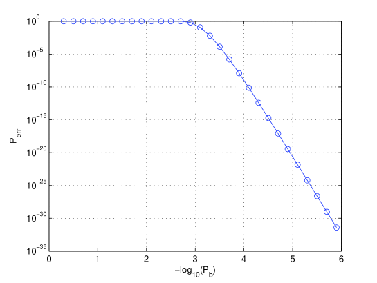
Figure 13: Probability of decoding error for the RS code $\mathcal{C}_{1024}[1023,1000]$ using bounded distance decoding.

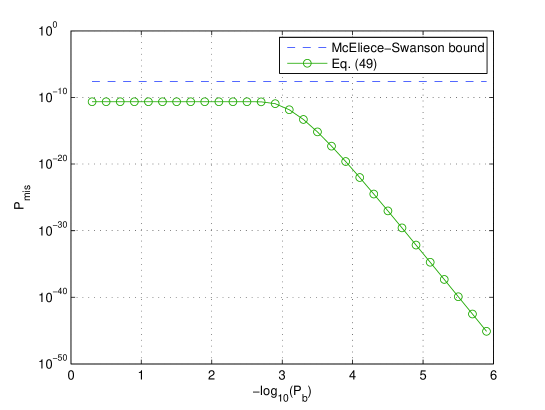
Figure 14: Probability of miscorrection for the RS code $\mathcal{C}_{1024}[1023,1000]$ using bounded distance decoding.

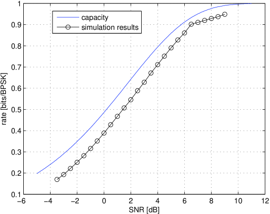
Figure 15: The average decoding rates of the Kite codes. The data length $k=50000$.

VI-B Construction Examples

We take RS code $\mathcal{C}_{1024}[1023,1000]$ over $\mathbb{F}_{1024}$ as the outer code. This code can correct up to $11$ symbol-errors. The performance of this code is shown in Fig. 13 and Fig. 14, respectively. Also shown in Fig. 14 is the McEliece-Swanson bound [44]. This computations can be used to predict the performance of the RS-Kite codes. For example, if the inner Kite code has an error-floor at $\textrm{BER}=10^{-4}$, then the outer RS code $\mathcal{C}_{1024}[1023,1000]$ can lower down this error-floor to $10^{-10}$ with miscorrection probability not greater than $10^{-20}$. This prediction is very reliable for large $\ell$.

We set $\ell=5$. Then the length of the input sequence to the inner code is 51150. We take Kite code $\mathcal{K}[\infty,51150;\underline{p}]$ as the inner code. The $p$-sequence is specified by

$$p_{t}=\left\{\begin{array}[]{rl}q_{9}=0.00084,&0.9\leq k/(t+k)<1.0\\ q_{8}=0.00020,&0.8\leq k/(t+k)<0.9\\ q_{7}=0.00015,&0.7\leq k/(t+k)<0.8\\ q_{6}=0.00009,&0.6\leq k/(t+k)<0.7\\ q_{5}=0.00006,&0.5\leq k/(t+k)<0.6\\ q_{4}=0.00006,&0.4\leq k/(t+k)<0.5\\ q_{3}=0.00004,&0.3\leq k/(t+k)<0.4\\ q_{2}=0.00002,&0.2\leq k/(t+k)<0.3\\ q_{1}=0.00001,&0.1\leq k/(t+k)<0.2\\ \end{array}\right..$$ (50)

The simulation results are shown in Fig. 15, where the error probability for each simulated point is upper-bounded by $P_{mis}$ because the receivers will try decoding with increasing redundancies until all RS codewords are decoded successfully. In our simulations, we have not observed any decoding errors. It can be seen from Fig. 15 that the gaps between the average decoding rates and the capacities are around $0.1$ bits/BPSK in the SNR range of $-3.0\sim 9.0$ dB. To our best knowledge, no simulation results were reported in the literature to illustrate that one coding method can produce good codes in such a wide range. We have also observed that there is a “singular” point at rate of $0.9$. This is because we have taken $0.9$ as the first target rate. If we add one more target rate of $0.95$, we can make this curve more smooth. But the other $q$-parameters need to be re-selected and the whole curve will change.

VII Conclusion

In this paper, we have proposed a new class of rateless forward error correction codes which can be applied to AWGN channels. The codes consist of RS codes and Kite codes linked in a serial concatenation manner. The inner Kite codes can generate potentially infinite parity-check bits with linear complexity. The use of RS codes as outer codes not only lowers down the error-floors but also ensures with high probability the correctness of the successfully decoded codewords. A semi-analytic method has been proposed to predict the error-floors of the proposed codes, which has been verified by numerical results. Numerical results also show that the proposed codes perform well over AWGN channels in a wide range of SNRs in terms of the gap to the channel capacity.

References

- [1] G. D. Forney, Jr., Concatenated Codes. Cambridge, MA: MIT Press, 1966.
- [2] D. J. Costello, Jr., J. Hagenauer, H. Imai, and S. B. Wicker, “Applications of error-control coding,” IEEE Trans. Inform. Theory, vol. 44, pp. 2531–2560, Oct. 1998.
- [3] C. Berrou, A. Glavieux, and P. Thitimajshima, “Near Shannon limit error-correcting coding and decoding: Turbo-codes,” in Proc. IEEE Int. Conf. on Communications, (Geneva, Switzerland), pp. 1064–1070, May 1993.
- [4] R. G. Gallager, Low-Density Parity-Check Codes. Cambridge, MA: MIT Press, 1962.
- [5] “Forward error correction for high bit-rate DWDM submarine systems.” ITU-T Recommendation G.975.1, Feb. 2004.
- [6] “Digital video broadcasting (DVB): Second generation framing structure, channel coding and modulation systems for broadcasting, interactive services, news gathering and other broad-band satellite applications.” EN 302 307, European Telecommunications Standards Institute (ETSI), 2006.
- [7] J. Byers, M. Luby, M. Mitzenmacher, and A. Rege, “A digital fountain approaches to reliable distribution of bulk data,” in Proc. ACM SIGCOMM’98, (Vancouver, BC, Canada), pp. 56–67, Jan. 1998.
- [8] M. Luby, “LT-codes,” in Proc. 43rd Annu. IEEE Symp. Foundations of computer Science (FOCS), (Vancouver, BC, Canada), pp. 271–280, Nov. 2002.
- [9] A. Shokrollahi, “Raptor codes,” IEEE Transactions on Information Theory, vol. 52, pp. 2551–2567, June 2006.
- [10] D. MacKay, “Fountain codes,” IEE Proc.-Commun., vol. 152, pp. 1062–1068, Dec. 2005.
- [11] R. Palanki and J. Yedidia, “Rateless codes on noisy channels,” in Proc. 2004 IEEE Int. Symp. Inform. Theory, (Chicago, IL), p. 37, Jun./Jul. 2004.
- [12] O. Etesami and A. Shokrollahi, “Raptor codes on binary memoryless symmetric channels,” IEEE Transactions on Information Theory, vol. 52, pp. 2033–2051, May 2006.
- [13] P. Pakzad and A. Shokrollahi, “Design principles for Raptor codes,” in Proc. 2006 IEEE Inform. Theory Workshop, (Punta del Este, Uruguay), pp. 165–169, March 2006.
- [14] G. P. Calzolari, M. Chiani, F. Chiaraluce, R. Garello, and E. Paolini, “Channel coding for future space missions: New requirements and trends,” Proceedings of The IEEE, vol. 95, pp. 2157–2170, Nov. 2007.
- [15] J. Hagenauer, “Rate-compatible punctured convolutional codes (RCPC codes) and their application,” IEEE Trans. Commun., vol. 36, pp. 389–400, April 1988.
- [16] G. Caire, T. Taricco, and E. Biglieri, “Bit-interleaved coded modulation,” IEEE Trans. Inform. Theory, vol. 44, pp. 927–946, May 1998.
- [17] A. Goldsmith, Wireless Communications. U.K.: Cambridge University Press, 2005.
- [18] N. Shulman, Universal Channel Coding. Ph.D. thesis, Tel-Aviv University, 2004.
- [19] F. R. Kschischang, B. J. Frey, and H.-A. Loeliger, “Factor graphs and the sum-product algorithm,” IEEE Trans. Inform. Theory, vol. 47, pp. 498–519, Feb. 2001.
- [20] G. D. Forney Jr., “Codes on graphs: Normal realizations,” IEEE Trans. Inform. Theory, vol. 47, pp. 520–548, February 2001.
- [21] S. Shamai, I. E. Telatar, and S. Verdú, “Fountain capacity,” IEEE Trans. Inform. Theory, vol. 53, pp. 4372–4376, Nov. 2007.
- [22] M. Luby, M. Mitzenmacher, A. Shokrollahi, D. Spielman, and V. Stemann, “Practical loss-resilient codes,” in Proc. 29th Annu. ACM Symp. Theory of Computing, pp. 150–159, 1997.
- [23] T. Richardson and R. Urbanke, “The capacity of low-density parity check codes under message-passing decoding,” IEEE Trans. Inform. Theory, vol. 47, pp. 599–618, February 2001.
- [24] J. Garcia-Frias and W. Zhong, “Approaching Shannon performance by iterative decoding of linear codes with low-density generator matrix,” IEEE Communications Letters, vol. 7, pp. 266–268, June 2003.
- [25] H. Jin, A. Khandekar, and R. McEliece, “Irregular repeat-accumulate codes,” in Proc. 2nd Intern. Symp. on Turbo Codes and Related Topics, pp. 1–8, Sept. 2000.
- [26] M. Yang, W. E. Ryan, and Y. Li, “Design of efficiently encodable moderate-length high-rate irregular LDPC codes,” IEEE Transactions on Communications, vol. 52, pp. 564–571, April 2004.
- [27] G. Liva, E. Paolini, and M. Chiani, “Simple reconfigurable low-density parity-check codes,” IEEE Communications Letters, vol. 9, pp. 258–260, March 2005.
- [28] A. Abbasfar, D. Divsalar, and K. Yao, “Accumulate-repeat-accumulate codes,” Communications, IEEE Transactions on, vol. 55, pp. 692 –702, April 2007.
- [29] X. Yuan, R. Sun, and L. Ping, “Simple capacity-achieving ensembles of rateless erasure-correcting codes,” IEEE Trans. Commun., vol. 58, pp. 110–117, Jan. 2010.
- [30] T. Richardson, A. Shokrollahi, and R. Urbanke, “Design of capacity-approaching low-density parity-check codes,” IEEE Trans. Inform. Theory, vol. 47, pp. 619–637, February 2001.
- [31] K. Price and R. Storn, “Differential evolution a simple and efficient heuristic for global optimization over continuous spaces,” J. Global Optimiz., vol. 11, pp. 341–359, 1997.
- [32] S. Benedetto, D. Divsalar, G. Montrosi, and F. Pollara, “Algorithm for continuous decoding of turbo codes,” Electronics Letters, vol. 32, pp. 314–315, February 1996.
- [33] R. J. McEliece, “On the BCJR trellis for linear block codes,” IEEE Trans. Inform. Theory, vol. 42, pp. 1072–1092, July 1996.
- [34] D. Divsalar, “A simple tight bound on error probability of block codes with application to turbo codes,” in Proc. 1999 IEEE Communication Theory Workshop, (Aptos, CA), May 1999.
- [35] D. Divsalar and E. Biglieri, “Upper bounds to error probabilities of coded systems beyond the cutoff rate,” IEEE Trans. Commun., vol. 51, pp. 2011–2018, Dec. 2003.
- [36] X. Ma, C. Li, and B. Bai, “Maximum likelihood decoding analysis of LT codes over AWGN channels,” in Proc. of the 6th International Symposium on Turbo Codes and Iterative Information Processing, (Brest, France), September 2010.
- [37] I. Sason and S. Shamai, “Performance analysis of linear codes under maximum-likelihood decoding: A tutorial,” in Foundations and Trends in Communications and Information Theory, vol. 3, pp. 1–225, Delft, The Netherlands: NOW, July 2006.
- [38] R. L. Rardin, Optimization in Operations Research. Englewood Cliffs, NJ: Prentice-Hall, 1998.
- [39] Y.-C. Ho, “An explanation of ordinal optimization: Soft computing for hard problems,” Inf. Sci., vol. 113, pp. 169–192, Feb. 1999.
- [40] S.-Y. Chung, T. Richardson, and Urbanke, “Analysis of sum-product decoding of low-density parity-check codes using gaussian approximation,” vol. 47, pp. 619–637, Feb 2001.
- [41] T. K. Moon, Error Correction Coding: Mathematical Methods and Algorithms. Hoboken, New Jersey: John Wiley & Sons, Inc., 2005.
- [42] B. Bai, B. Bai, and X. Ma, “Semi-random kite codes over fading channels,” in Proc. IEEE International Conference on Advanced Information Networking and Applications (AINA), (Biopolis, Singapore), pp. 639–645, March 2011.
- [43] S. Lin and D. J. Costello Jr., Error Control Coding: Fundamentals and Applications. Englewood Cliffs, NJ: Prentice-Hall, second ed., 2004.
- [44] R. J. McEliece and L. Swanson, “On the decoder error probability for Reed-Solomon codes,” IEEE Transactions on Information Theory, vol. IT-32, pp. 701–703, Sept. 1986.
- [45] I. Sofair, “Probability of miscorrection for Reed-Solomon codes,” in Proc. International Conference on Information Technology: Coding and Computing, (Las Vegas, Nevada), pp. 398–401, March 2000.
- [46] E. Paaske, “Improved decoding for a concatenated coding system recommended by CCSDS,” IEEE Trans. Commun., vol. 38, pp. 1138–1144, Aug. 1990.
- [47] O. Collins and M. Hizlan, “Determinate-state convolutional codes,” IEEE Trans. Commun., vol. 41, pp. 1785–1794, Dec. 1993.