Photon-number entangled states generated in Kerr media with optical parametric pumping

Abstract

Two nonlinear Kerr oscillators mutually coupled by parametric pumping are studied as a source of states entangled in photon numbers. Temporal evolution of entanglement quantified by negativity shows the effects of sudden death and birth of entanglement. Entanglement is preserved even in asymptotic states under certain conditions. The role of reservoirs at finite temperature in entanglement evolution is elucidated. Relation between generation of entangled states and violation of Cauchy-Schwartz inequality for oscillator intensities is found.

I Introduction

Generation of entangled states and their protection from disentanglement is a crucial task in quantum information processing theory. Entangled states can be generated in various physical systems. Entanglement can be observed in various degrees of freedom. The most common systems considered as sources of entangled states are spin systems (NMR), quantum dotsLV98 , trapped ions CZ95 , double-well Bose-Einstein condensates VPA04 . Typical constituents of these systems can be represented by two (or more) level atoms that mutually interact and create this way entangled states. We speak about systems composed of qubits (see for example F10 and the references quoted therein), qutrits or higher dimensional qudits. On the other hand, entangled states can be found also in field systems, namely in optical fields. Entanglement emerges here due to mutual interaction among modes of optical fields. This interaction typically occurs in nonlinear optical processes Boyd2003 . Entanglement can then be observed in polarization states (for example PHJ94 ) or photon-number states Bouwmeester2000 . Namely states entangled in photon numbers are promising for the near future due to the progress in construction of photon-number resolving detectors in the last years. Their construction can be based on optical-fiber loop interferometers Rehacek2003 ; Achilles2004 ; Fitch2003 , absorption in superconductor wires Miller2003 , use of intensified CCD cameras Haderka2005 ; Hamar2010 , complex semiconductor structures Kim1999 or hybrid photodetectors Bondani2009 .

Every real physical system interacts with its environment Fick1990 . Such interaction leads to losses of coherence, and consequently, to gradual degradation of entanglement. In quantum information processing this represents one of the crucial problems. That is why many methods for coping with this problem have been developed; quantum error correction S95 ; EM96 ; G96 ; CRSS97 , decoherence free subspaces PSE96 ; DG98 ; LW03 , proper preparation of qubit states ZR98 , multiple system-decomposition method JD08 , to name few. It is well known that an entangled state interacting with a zero temperature Markovian environment asymptotically decays in time. However the character of zero-temperature reservoir decay can be altered. Under specific conditions disentanglement may suddenly occur (sudden death of entanglement) ZHHH01 ; D03 ; YE04 . Moreover, if a system interacts with a thermal or squeezed ILZ07 reservoir the entanglement is lost in finite time as well. We should also mention that the effect of sudden entanglement birth can also be observed FT06 ; FT08 ; LRLSR08 .

In this paper, we consider two optical modes generated by parametric down-conversion Mandel1995 pumped by an intense optical field. The generated two optical modes propagate through a medium characterized by Kerr nonlinearity that modifies their statistical properties. States characterizing two optical modes can be entangled in photon numbers (see for example PHJ94 ) as a consequence of the fact that photons are emitted in pairs in parametric down-conversion. Provided that interaction with external reservoir is taken into account the effects of sudden death and sudden birth of entanglement can be observed. Entanglement will be quantified by negativity function and its presence will be compared with nonclassical behavior of distributions of integrated intensities of two modes. We note that experimental characterization of nonclassical two-mode optical fields is experimentally available PKPBAA09 .

Optical fibers are suitable candidates for experimental generation of the predicted entangled states. They allow both the generation of photon pairs in parametric processes Li2005 ; Fulconis2005 and exhibit Kerr nonlinearities Sizmann1999 . Nonlinear fibers allow to generate sufficiently high photon-pair fluxes. For example, a nonlinear fiber $300$ m long embedded into a Sagnac interferometer allows to generate up to $10^{7}$ photon pairs per $1$ mW of optical pumping Li2005 . Similar photon-pair generation rates have also been reported from a 2 m long micro-structured fiber Fulconis2005 .

However, we note that nonlinear systems excited directly by an external coherent field [referred as nonlinear quantum scissors ML06 ; KL06 ; KL09 ] require giant Kerr nonlinearities that can be achieved, e.g., using induced transparency KZ03 ; BC08 ; SRKD08 .

The paper is organized as follows. A quantum model of two interacting optical fields is formulated and solved in Sec. II that also contains considerations about entanglement. Generalization of the model to the case of interaction with reservoir is provided in Sec. III. Nonclassical behavior of integrated intensities of two modes is discussed in Sec. IV. Sec. V provides conclusions.

II The model, its solution and entanglement evolution

The considered system is composed of nonlinear medium (characterized by Kerr nonlinearity) that is excited by an external field of strength $g$. At quantum level, two photons (belonging to different field modes) are emitted together in the parametric process. Interaction Hamiltonian $\hat{H}_{int}$ of the system can be written in the following form:

$$\hat{H}_{\rm int} = \hat{H}_{\rm Kerr}+\hat{H}_{\rm par}$$ (1)

$$\hat{H}_{\rm Kerr} = \frac{\chi_{a}}{2}(\hat{a}^{\dagger})^{2}\hat{a}^{2}+\frac{\chi_{b}}{2}(\hat{b}^{\dagger})^{2}\hat{b}^{2},$$ (2)

$$\hat{H}_{\rm par} = g\hat{a}^{\dagger}\hat{b}^{\dagger}+g^{\star}\hat{a}\hat{b}.$$ (3)

Here, Hamiltonian $\hat{H}_{\rm Kerr}$ describes two nonlinear Kerr oscillators (with nonlinearities $\chi_{a,b}$) whereas Hamiltonian $\hat{H}_{\rm par}$ means an effective interaction Hamiltonian of the two-mode parametric process P91 . Model Hamiltonians including both parametric and Kerr processes have been analysed in PP00 . It should be noted that our model does not include the Kerr cross term $\hat{a}^{\dagger}\hat{a}\hat{b}^{\dagger}\hat{b}$, that is important in some Kerr media (for discussion concerning models involving such Kerr cross term see, for example KP96 ; *KP97; CSKSL98 and the references quoted therein). We note that the Hamiltonian analogous to that considered here has also been used for example, by Bernstein Bernstein93 or Chefles and Barnett CheflesBarnett96 . The dynamics of the models excluding the Kerr cross term have also been analyzed in other papers, for instance in AbdelBaset00 ; Olsen06 .

It should be stressed out that various interesting effects beside of those discussed in the quantum information theory can originate in systems endowed with Kerr nonlinearities. For instance, Miranowicz at al. MTK90 have shown that discrete superpositions of an arbitrary number of coherent states (so-called Schrödinger cat-like or kitten states) can be generated in these systems. Moreover, such nonlinear systems (especially, nonlinear couplers with Kerr nonlinearities ML06 ; KL06 ; KL09 ) can serve as a source of maximally entangled states (MES) useful not only in quantum optics but also in other branches of physics. For instance, Kurpas et al. KDZ09 discussed nonlinear resonances and entanglement generation in solid state models, particularly in those involving SQUID systems.

At the beginning we neglect damping. That is why we simply apply the Schr$\ddot{o}$dinger equation that can be written in the form of a set of equations for complex probability amplitudes $c_{nm}(t)$ corresponding to the Fock state with $n$ photons in mode $a$ and $m$ photons in mode $b$. Assuming that the initial state is the vacuum state in both modes $|\Psi(t=0)\rangle=|0\rangle_{a}|0\rangle_{b}$ these equation can be obtained in the form (we use units of $\hbar=1$):

$$i\frac{d}{dt}c_{nm} = \frac{1}{2}\left\{n(n-1)\chi_{a}+m(m-1)\chi_{b}\right\}c_{nm}$$ (4)

$$\mbox{}+g\sqrt{nm}\,\,c_{n-1,m-1}$$

$$\mbox{}+g^{\star}\sqrt{(n+1)(m+1)}\,\,c_{n+1,m+1}.$$

Inspection of the form of Eqs. (4) leads to the conclusion that the dynamics of the system is not restricted to a closed set of two-mode states. The number of states involved considerably in the dynamics depends straightforwardly on the level of excitation $g$ - the larger the value of $g$ the larger the number of involved states. Assuming the initial vacuum state ($|\Psi(t=0)\rangle=|0\rangle_{a}|0\rangle_{b}$) and lossless dynamics only two-mode states having equal photon numbers in modes $a$ and $b$ are involved in the dynamics.

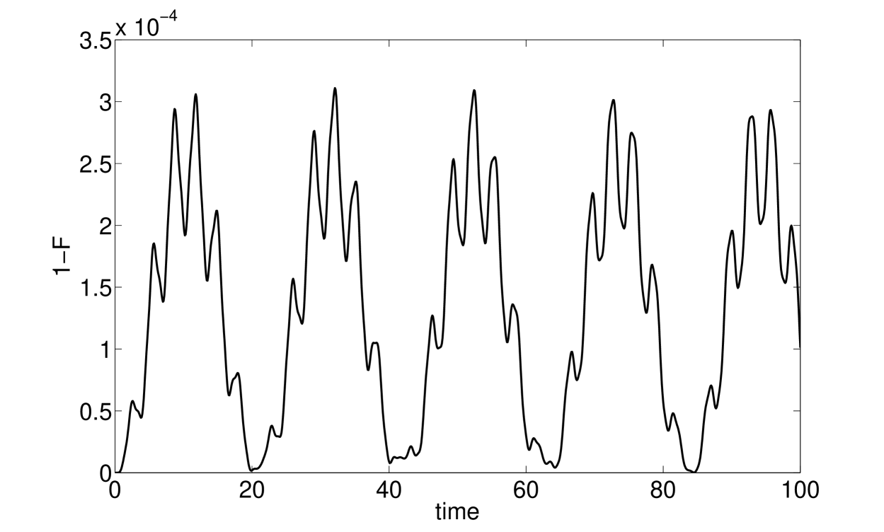
Figure 1: Declination of fidelity $F$ from unity as a function of scaled time $t$. Fidelity $F$ is calculated between the state defined in the subspace spanned by states $|0\rangle_{a}|0\rangle_{b}$, $|1\rangle_{a}|1\rangle_{b}$, and $|2\rangle_{a}|2\rangle_{b}$ and the state evolving in the subspace containing states $|i\rangle_{a}|j\rangle_{b}$ for $i,j=0,\ldots,10$. The scaled time $t$ is measured in $1/\chi_{a,b}$ units. Initial vacuum state $|0\rangle_{a}|0\rangle_{b}$ is assumed, $g=0.15$.

To be more specific, the number of states that must be considered depends on the value of ratio $r=g/(\chi_{a}+\chi_{b})$ and length of the time-evolution. For small values of $r<0.1$ the conditions resemble those discussed in ML06 ; KL06 ; KL09 where nonlinear quantum scissors have been studied. In this case, only states with small photon numbers in both modes $a$ and $b$ are involved. In particular, we can restrict the dynamics of the system to just first three lowest states of the whole set of two-mode states: $|0\rangle_{a}|0\rangle_{b},|1\rangle_{a}|1\rangle_{b},|2\rangle_{a}|2\rangle_{b}$. Validity of this approximation can be judged comparing the approximative solution with the full (numerical) solution. Fidelity between the two states has been found useful in this case. A typical example investigated in Fig. 1 shows that the dynamics of the whole system can be restricted to the subspace of three states with accuracy of order $3\times 10^{-4}$. For this case we assume that $g=0.15$. This value seems to be the optimal one, since it is small enough to keep the system’s evolution closed within the desired range of the states and to derive the analytical formulas for the dynamics. Simultaneously, the value $g=0.15$ is sufficient to observe the Bell-states generation. The reason is that if we assume the value for $g$ to be too small, mostly the vacuum state is populated and an efficient Bell-state generation is not possible.

In this approximation, the evolution of probability amplitudes is governed via the equations:

$$i\frac{d}{dt}c_{00}(t) = g^{\star}c_{11}(t)$$

$$i\frac{d}{dt}c_{11}(t) = gc_{00}(t)+2g^{\star}c_{22}(t)$$

$$i\frac{d}{dt}c_{22}(t) = 2gc_{11}(t)+Ac_{22}(t),$$ (5)

where $A=\chi_{a}+\chi_{b}$.

The solution of Eqs. (5) can be obtained analytically:

$$c_{00}(t) = r_{01}\exp{(s_{1}t)}+r_{02}\exp{(s_{2}t)}+r_{03}\exp{(s_{3}t)}$$

$$c_{11}(t) = r_{11}\exp{(s_{1}t)}+r_{12}\exp{(s_{2}t)}+r_{13}\exp{(s_{3}t)}$$

$$c_{22}(t) = r_{21}\exp{(s_{1}t)}+r_{22}\exp{(s_{2}t)}+r_{23}\exp{(s_{3}t)},$$

where

$$s_{1} = \frac{ig}{3x}\left(-1+\frac{1+15x^{2}}{M}+M\right),$$

$$s_{2} = \frac{g}{6x}\left(-2i-X_{2}/M\right)\,,$$

$$s_{3} = \frac{g}{6x}\left(-2i+X_{2}^{\star}/M\right)\,.$$ (7)

Amplitudes $r_{ij}$ take the following form:

$$r_{01} = \frac{12x}{m_{1}}\Bigl{[}-ix(7+75x^{2})+K+M(-2ix+K)$$

$$\mbox{}+2ixM^{2}\Bigr{]},$$

$$r_{02} = \frac{x}{m_{2}}\Bigl{[}(-3-i\sqrt{3})(7+75x^{2})x+(-3i+\sqrt{3})K$$

$$\mbox{}+2(3-i\sqrt{3})xM+(3i+\sqrt{3})KM-4\sqrt{3}ixM^{2}\Bigr{]},$$

$$r_{03} = \frac{x}{m_{3}}\Bigl{[}(3-i\sqrt{3})(7+75x^{2})x+(3i+\sqrt{3})K$$

$$\mbox{}-2(3+i\sqrt{3})xM+(-3i+\sqrt{3})KM-4\sqrt{3}ixM^{2}\Bigr{]},$$

$$r_{11} = \frac{12ixM}{m_{1}}\left(15x^{2}+(1+M)^{2}\right),$$

$$r_{12} = -r_{13}^{\star}=\frac{\sqrt{3}xM}{m_{2}}\left(X_{2}-4iM\right),$$

$$r_{21} = -\frac{72ix^{2}M^{2}}{m_{1}},$$

$$r_{22} = \frac{12i\sqrt{3}x^{2}M^{2}}{m_{2}},$$

$$r_{23} = r_{22}\frac{m_{2}}{m_{3}}.$$ (8)

Denominators occurring in Eqs. (8) for amplitudes are given as:

$$m_{1} = \left|X_{1}\right|^{2},$$

$$m_{2} = m_{3}^{\star}=\left(-1-15x^{2}+M^{2}\right)X_{1}.$$ (9)

Also the following parameters have been used in the above relations:

$$X_{1} = (3i-\sqrt{3})(1+15x^{2})+(3i+\sqrt{3})M^{2},$$

$$X_{2} = (i-\sqrt{3})(1+15x^{2})+(i+\sqrt{3})M^{2},$$

$$M = \left(-1-9x^{2}+3ixK\right)^{1/3},$$

$$K = \sqrt{3+66x^{2}+375x^{4}},$$

$$x = g/(\chi_{a}+\chi_{b}).$$ (10)

The analytical solution in Eqs. (LABEL:amp_smg_sol) valid for three two-mode states allows to analyze entanglement in the system. Here, we pay attention to qubit-qubit entanglement and quantify it using negativity. This entanglement measure is defined as Peres ; Horodecki96 :

$$N(\hat{\rho})=\max\Big{(}0,-2\min_{j}\mu_{j}\Big{)},$$ (11)

where $\mu_{j}$ are the eigenvalues of the partial transpose of the density matrix $\hat{\rho}^{\Gamma}$. The factor $2$ appearing in this definition is chosen to get $N(\hat{\rho})=1$ for Bell’s states. Negativity is a commonly used entanglement measure allowing the entanglement quantification – for maximally entangled state we have $N(\hat{\rho})=1$, whereas $N(\hat{\rho})=0$ occurs for the cases when the entanglement disappears completely. Moreover, it can be applied for more general models exceeding the simple qubit-qubit one.

In our system, we can define three subsystems of the qubit-qubit form: the first subsystem is spanned by the states $|0\rangle_{a}|0\rangle_{b}$ and $|1\rangle_{a}|1\rangle_{b}$ (negativity $N_{0110}$), the second one by states $|0\rangle_{a}|0\rangle_{b}$ and $|2\rangle_{a}|2\rangle_{b}$ (negativity $N_{0220}$) and the third one by states $|1\rangle_{a}|1\rangle_{b}$ and $|2\rangle_{a}|2\rangle_{b}$ (negativity $N_{1221}$). We note that these subsystems are not independent – each of the two-mode states is involved in two considered qubit-qubit subsystems. This also means that there occur correlations in the presence of entanglement in these subsystems.

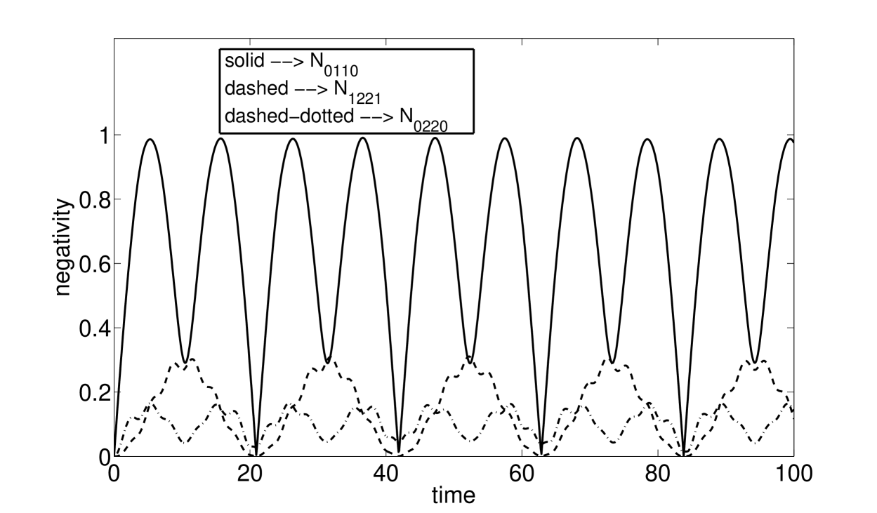
Figure 2: Negativities $N_{0110}$, $N_{0220}$, and $N_{1221}$ as functions of scaled time $t$ measured in $1/\chi_{a,b}$ units. The coupling $g=0.15$, other parameters and used units are the same as in caption to Fig. 1.

This is illustrated in Fig. 2, where the negativities $N_{0110}$, $N_{0220}$, and $N_{1221}$ for the subsystems are plotted. Negativity $N_{0220}$ oscillates with a relatively small amplitude (around the value of $0.17$) similarly as negativity $N_{1221}$ (having the amplitude around $0.3$). On the other hand, values of negativity $N_{0110}$ show that the system can be treated as a generator of Bell states in certain time instants in which $N_{0110}\approx 1$. The generated Bell states are of the form:

$$|B_{1}\rangle = \frac{1}{\sqrt{2}}\left(|0\rangle_{a}|0\rangle_{b}+i|1\rangle_{a}|1\rangle_{b}\right),$$

$$|B_{2}\rangle = \frac{1}{\sqrt{2}}\left(|0\rangle_{a}|0\rangle_{b}-i|1\rangle_{a}|1\rangle_{b}\right).$$ (12)

Moreover, whenever negativity $N_{0110}$ achieves the shallower minimum (with amplitude approx.$\sim 0.3$), entanglement is partially transferred to the subsystem spanned by states $|1\rangle_{a}|1\rangle_{b}$ and $|2\rangle_{a}|2\rangle_{b}$ $\{1221\}$. In addition, when negativity $N_{0110}$ equals zero negativity $N_{1221}$ also vanishes. However, the whole system is not in a pure state in this specific case because $N_{0220}\neq 0$. The values of negativity $N_{1221}$ are not high for a fixed value of $g$, but we have observed that the mechanism of entanglement transfer alters as $g$ increases. At larger values of $g$ temporal evolution of negativities $N_{0110}$, $N_{0220}$, and $N_{1221}$ is more complex (see Fig. 3a). In particular, the role of higher populated two-mode states ($|2\rangle_{a}|2\rangle_{b}$) is more pronounced and entanglement in subsystem composed of states $|0\rangle_{a}|0\rangle_{b}$ and $|1\rangle_{a}|1\rangle_{b}$ is weaker. There occur time instants in which negativity $N_{0110}$ achieves one of its minima and nearly simultaneously entanglements in other both subspaces reach their maximal values. For comparison, we have drawn in Fig. 3 also parameter $R$ that quantifies the violation of Cauchy-Schwartz inequality (CSI, for definition, see later) and serves as a measure of non-classicality of the whole system.

Inspection of curves in Fig. 3 indicates that maximum of parameter $R$ can be reached in time instants in which qubit-qubit negativities are far from their maximal values. This reflex complexity of quantum states found in temporal evolution of the discussed system. It should be noted that, for the case discussed here, we have assumed the greater value of parameter $g$. The used value $g=0.6$ has been found optimal for the entanglement generation within the considered qubit-qubit subsystem. However, the states involving more than two photons are non-negligibly populated and so we cannot apply the analytical formulas derived above.

III Entanglement generation in damped reservoir

As any real physical system is not completely isolated, we should include into considerations about entanglement formation and its time-evolution also environmental effects. We describe damping in the standard Born and Markov approximations. We thus apply the following master equation for the reduced statistical operator $\hat{\rho}$:

$$\frac{d}{dt}\hat{\rho} = -i(\hat{H}\hat{\rho}-\hat{\rho}\hat{H})+\gamma_{a}\left[\hat{a}\hat{\rho}\hat{a}^{\dagger}-\frac{1}{2}\left(\hat{\rho}\hat{a}^{\dagger}\hat{a}+\hat{a}^{\dagger}\hat{a}\hat{\rho}\right)\right]$$ (13)

$$\mbox{}+\bar{n}_{a}\gamma_{a}\left[\hat{a}^{\dagger}\hat{\rho}\hat{a}+\hat{a}\hat{\rho}\hat{a}^{\dagger}-\hat{a}^{\dagger}\hat{a}\hat{\rho}-\hat{\rho}\hat{a}\hat{a}^{\dagger}\right]$$

$$\mbox{}+\gamma_{b}\left[\hat{b}\hat{\rho}\hat{b}^{\dagger}-\frac{1}{2}\left(\hat{\rho}\hat{b}^{\dagger}\hat{b}+\hat{b}^{\dagger}\hat{b}\hat{\rho}\right)\right]$$

$$\mbox{}+\bar{n}_{b}\gamma_{b}\left[\hat{b}^{\dagger}\hat{\rho}\hat{b}+\hat{b}\hat{\rho}\hat{b}^{\dagger}-\hat{b}^{\dagger}\hat{b}\hat{\rho}-\hat{\rho}\hat{b}\hat{b}^{\dagger}\right],$$

where $\gamma_{a,b}$ are damping constants and $\bar{n}_{a,b}$ denote mean photon numbers of noise in modes $a$ and $b$.

Operator equation written in Eq. (13) can be transformed into the following differential equations of motions for the elements $\rho_{n\,m,k\,l}$ of statistical operator; $\rho_{n\,m,k\,l}\equiv\langle k|\langle n|\rho|m\rangle|l\rangle$:

$$\frac{d}{dt}\rho_{n\,m,k\,l} = -\frac{1}{2}\Bigl{[}i\chi_{a}\left(n(n-1)-m(m-1)\right)$$ (14)

$$\mbox{}+i\chi_{b}\left(k(k-1)-l(l-1)\right)$$

$$\mbox{}+\gamma_{a}\left(n+m-2\bar{n}_{a}(n+m+1)\right)$$

$$\mbox{}+\gamma_{b}\left(k+l-2\bar{n}_{b}(k+l+1)\right)\Bigr{]}\rho_{n\,m,k\,l}$$

$$\mbox{}+g\sqrt{nk}\;\,\rho_{n-1\,m,k-1\,l}$$

$$\mbox{}-g\sqrt{(m+1)(l+1)}\;\,\rho_{n\,m+1,k\,l+1}$$

$$\mbox{}+g^{\star}\sqrt{(n+1)(k+1)}\;\,\rho_{n+1\,m,k+1\,l}$$

$$\mbox{}-g^{\star}\sqrt{ml}\;\,\rho_{n\,m-1,k\,l-1}$$

$$\mbox{}+\gamma_{a}\Bigl{(}1+\bar{n}_{a})\sqrt{(n+1)(m+1)}\;\,\rho_{n+1\,m+1,k\,l}$$

$$\mbox{}+\bar{n}_{a}\sqrt{nm}\;\,\rho_{n-1\,m-1,k\,l}\Bigr{]}$$

$$\mbox{}+\gamma_{b}\Bigl{[}(1+\bar{n}_{b})\sqrt{(k+1)(l+1)}\;\,\rho_{n\,m,k+1\,l+1}$$

$$\mbox{}+\bar{n}_{b}\sqrt{kl}\;\,\rho_{n\,m,k-1\,l-1}\Bigr{]}.$$

In numerical calculations, the number of equations in Eq. (14) that have to be considered depends strongly on the value of constant $g$: the larger the value of $g$ the greater the number of equations.

III.1 Zero-temperature reservoir

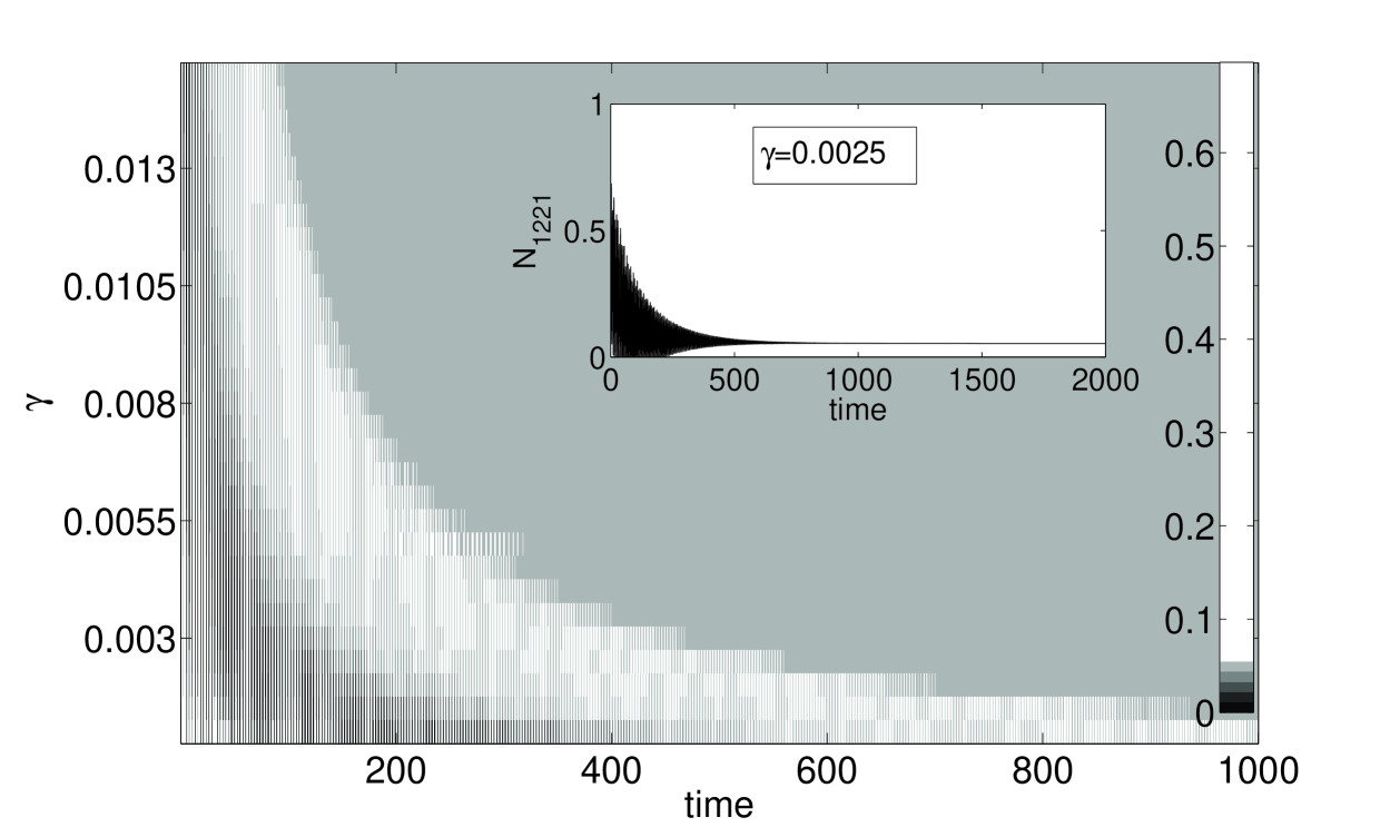
Figure 4: Map of negativity $N_{1221}$ as a function of scaled in $1/\chi_{a,b}$ units time $t$ and damping $\gamma$ (measured in $\chi_{a,b}$ units). Nonzero values of negativity $N_{1221}$ occur inside grey and black areas. In the inset temporal evolution of negativity $N_{1221}$ for $\gamma=0.0025$ is shown. The coupling $g=0.6$, other parameters and units are the same as in caption to Fig. 3.

The zero-temperature reservoir is defined by the requirement that mean number of photons is zero, i.e. the system is influenced only by vacuum fluctuations of the environment. In the analysis we restrict ourselves to the subspace that contains states with no more than two photons in mode $a$ and $b$. We have found for the case discussed here that some amount of entanglement described by negativities occurs in the system regardless on the damping strengths $\gamma_{a,b}$. It is documented in Fig. 4 where the map of negativity $N_{1221}$ as a function of time $t$ and damping constant $\gamma$ is plotted ($\gamma\equiv\gamma_{a}=\gamma_{b}$).

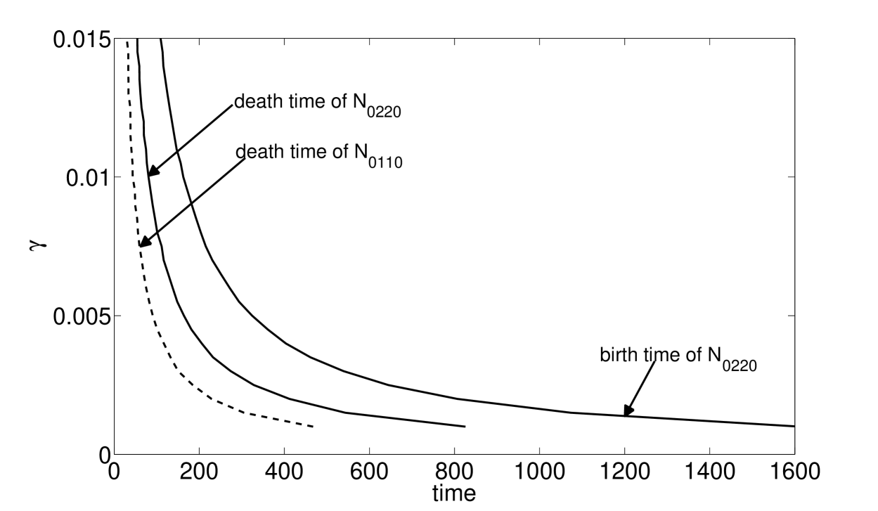
Figure 5: Borders between the regions with zero/nonzero negativities $N_{0110}$ (dashed curve) and $N_{0220}$ (solid curves) at the time axis as they depend on damping $\gamma$ (measured in $\chi_{a,b}$ units). The curves indicate instants in which the effects of sudden death and sudden birth of entanglement occur. In the area between two solid lines, no entanglement described by negativity $N_{0220}$ is found. The coupling $g=0.6$, other parameters and the units used here are the same as for Fig. 3.

A typical temporal evolution of negativity is such that after oscillations at the beginning an asymptotic nonzero value is reached (set the inset in Fig. 4). It is interesting to note that the asymptotic value does not depend on the level of damping (for $g=0.6$, $N_{1221}\sim 0.054$). On the other hand, negativity $N_{0110}$ shows that the effect of sudden death of entanglement occurs in the subsystem with zero and one photons in modes $a$ and $b$. Even more interestingly, negativity $N_{0220}$ of the subsystem composed of states $|0\rangle_{a}$, $|2\rangle_{a}$, $|0\rangle_{b}$, and $|2\rangle_{b}$ brings evidence of the effects of sudden death and sudden birth of entanglement. After entanglement rebirth negativity $N_{0220}$ reaches its nonzero asymptotic value ($N_{0220}\sim 0.035$ for $g=0.6$) regardless of the damping strength $\gamma$. Positions of the borders between zero and non-zero values of negativities $N_{0110}$ and $N_{0220}$ are plotted in Fig. 5. It is worth mentioning that entanglement described by negativity $N_{0220}$ lives almost two times longer before its sudden death compared to that described by negativity $N_{0110}$.

Analytical treatment enables to reveal the origin of the observed features to certain extent. If the system is not damped, the generated states are in a coherent superposition of states $|i\rangle_{a}|i\rangle_{b}$ containing $i$ photon pairs [compare the form of Hamiltonian $H_{\rm int}$ in Eq. (1)]. In a damped system, depopulation channels due to spontaneous emission are opened and, as a consequence, the system has to be described by statistical operator $\hat{\rho}$. Nevertheless, projected statistical operators $\hat{\rho}^{\rm red}$ of the considered qubit-qubit subsystems attain an ”X” type form:

$$\hat{\rho}^{\rm red}=\left(\begin{array}[]{cccc}a_{11}&0&0&a_{14}\\ 0&a_{22}&0&0\\ 0&0&a_{33}&0\\ a_{41}&0&0&a_{44}\end{array}\right).$$ (15)

In Eq. (15) elements $a_{ii}$ describe populations of the corresponding states whereas $a_{ij}$ ($i\neq j$) stand for coherences (probability flows).

The statistical operator $\hat{\rho}^{\rm red}$ written in Eq. (15) can be after partial transposition easily diagonalized. Its eigenvalues can be written as:

$$\lambda_{1} = a_{11},$$

$$\lambda_{2} = \frac{1}{2}\left[a_{22}+a_{33}-\sqrt{\left(a_{22}-a_{33}\right)^{2}+4a_{14}a_{41}}\right],$$

$$\lambda_{3} = \frac{1}{2}\left[a_{22}+a_{33}+\sqrt{\left(a_{22}-a_{33}\right)^{2}+4a_{14}a_{41}}\right],$$

$$\lambda_{4} = a_{44}.$$ (16)

Nonzero negativity $N$ occurs whenever at least one of the eigenvalues written in Eq. (16) is negative Hill1997 . The analysis of the formulas in Eq. (16) shows that this situation is found whenever $a_{22}a_{33}<a_{14}a_{41}$. The equality $a_{22}a_{33}=a_{14}a_{41}$ then represents the border condition that localizes the effects of sudden death and sudden birth of entanglement. A detailed discussion of the relation between the form of a statistical operator and conditions for entanglement vanishing or rebuilding can be found in the review article F10 .

In detail, negativity $N_{0110}$ is larger than zero provided that

$$\frac{\rho_{00,11}\rho_{11,00}}{\rho_{01,01}\rho_{10,10}}<1.$$ (17)

Similarly, the conditon

$$\frac{\rho_{00,22}\rho_{22,00}}{\rho_{02,02}\rho_{20,20}}<1$$ (18)

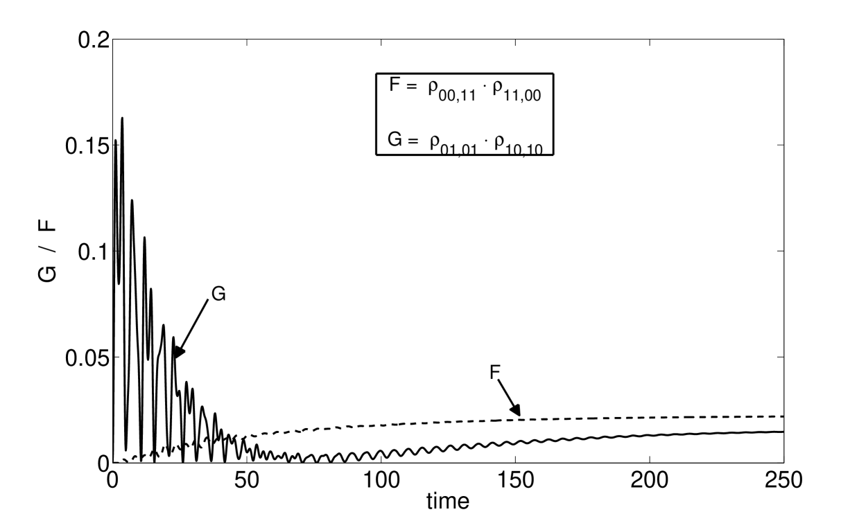
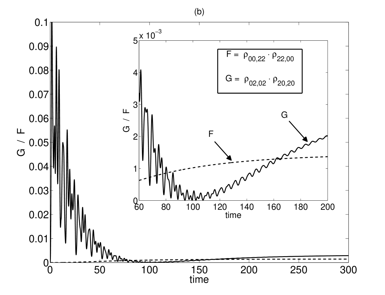
Figure 6: Time evolution of quantities $F$ ($F=\rho_{00,11}\rho_{11,00}$) and $G$ ($G=\rho_{01,01}\rho_{10,10}$) giving numerators and denominators, respectively, in conditions written in Eqs. (17) (a) and Eqs. (18). Crossing of the curves indicate instants of sudden death and sudden birth of entanglement. Inset in (b) shows a detail of temporal evolution; $\gamma=0.01$. The coupling $g=0.6$, other other parameters are the same as in caption to Fig. 3. Time $t$ is measured in $1/\chi_{a,b}$ units.

guarantees nonzero values of negativity $N_{0220}$. In general and roughly speaking, the conditions written in Eqs. (17) and (18) say that entanglement is lost at the moment when populations become larger than coherences. However, if coherences become larger than populations later, entanglement is revealed. This is documented in Fig. 6 for the evolution of entanglement in the subsystems described by negativities $N_{0110}$ and $N_{0220}$. Whereas the curves in Fig. 6 clearly identify the instant of sudden death of entanglement in case of negativity $N_{0110}$ (Fig. 6a), instants of both the sudden death and sudden birth of entanglement can be determined in case of negativity $N_{0220}$ (Fig. 6b).

We note that the explanation of occurrence of entanglement sudden death and sudden birth presented here is very similar to that discussed by Ficek and Tanaś in FT06 when investigating two two-level atoms in a cavity. They have shown that dark periods of entanglement are observed provided that the population of a symmetric state became larger than the appropriate coherences.

We would like to stress that, in our model, entanglement does not vanish in the long-time limit even for a damped system. Some parts of the whole system are disentangled as evidenced, e.g., by zero asymptotic values of negativity $N_{0110}$. However, there exist parts of the whole system that remain asymptotically entangled. Moreover, the study of temporal dynamics of entanglement has revealed that entanglement can “flow” among different subsystems. This may preserve entanglement from damping processes and its loss. We also note that the studied system does not evolve into a pure state which distinguishes it from many other systems that exhibit total disentanglement in the long-time limit.

III.2 Thermal reservoir damping

Considering a thermal reservoir at finite temperature, mean numbers $\bar{n}_{a}$ and $\bar{n}_{b}$ of reservoir photons are nonzero and so dynamics of the system is governed by the master equation in its general form given by Eq. (13). Unfortunately, such reservoirs lead to weakening of entanglement compared to the case of zero-temperature reservoirs discussed above.

Assuming smaller values of mean reservoir photon numbers $\bar{n}_{a}$ and $\bar{n}_{b}$, entanglement is generated in all three considered qubit-qubit subsystems, as described by negativities $N_{0110}$, $N_{0220}$, and $N_{1221}$ for finite times. Whereas entanglement indicated by negativities $N_{0110}$ and $N_{0220}$ arrives at the crucial points of sudden death, certain amount of asymptotic entanglement is preserved as evidenced by nonzero asymptotic values of negativity $N_{1221}$. It holds that the larger the mean reservoir photon-numbers $\bar{n}_{a}$ and $\bar{n}_{b}$, the smaller the asymptotic values of negativity $N_{1221}$ (see Fig. 7).

The dynamics of entanglement is in general more complex for finite-temperature reservoirs compared to those at zero temperature, as documented in Fig. 7 where many periods of entanglement sudden death and sudden birth occur in the evolution of negativity $N_{1221}$. We have also observed, that entanglement described by negativity $N_{0110}$ disappears approximately two times faster compared to that monitored by negativity $N_{0220}$. The instants of sudden death of entanglement depend strongly on damping constants $\gamma_{a}$ and $\gamma_{b}$: the larger the values of constants $\gamma_{a}$ and $\gamma_{b}$, the sooner the effect of sudden death occurs. Qualitatively the same dependence as that depicted in Fig. 5 for zero-temperature reservoirs has been revealed.

Asymptotic values of negativity $N_{1221}$ are zero for sufficiently large values of mean reservoir photon numbers $\bar{n}_{a}$ and $\bar{n}_{b}$. In this case, entanglement in the whole system is completely lost. In this case, also parameter $R$ describing violation of Cauchy-Schwartz inequality is smaller than one indicating classical behaviour of two modes.

We note that, similarly as in the case of zero-temperature reservoirs, entanglement is present whenever populations are larger than coherences.

Comparison with the model of a nonlinear coupler interacting with a thermal reservoir and excited by an external coherent field as analysed in KL09 underlines a distinguished property of this system - the ability to generate asymptotic entanglement at finite temperatures.

IV Nonclassical correlations of integrated intensities

Entanglement between fields in modes $a$ and $b$ has been monitored using negativity of different qubit-qubit subsystems defined inside modes $a$ and $b$. The presence of entanglement in at least one of the subsystems reflected entanglement between optical fields in these modes. We have observed that whenever the system shows entanglement also nonclassical correlations between integrated intensities of fields in modes $a$ and $b$ occur Perina2009 . These nonclassical correlations of intensities occur only provided that the joint quasi-distribution (in the form of a generalized function) of integrated intensities related to normal ordering of field operators attains negative values for some regions of intensities P91 . These negative values can be monitored, e.g., using second-order intensity correlation functions $\Gamma^{(2)}$ that violate the Cauchy-Schwartz inequality. Violation of this inequality can be quantified using parameter $R$ defined a LYXLY06 :

$$R(t)=\frac{\Gamma^{(2)}_{a,b}(t)}{\sqrt{\Gamma^{(2)}_{a,a}(t)\Gamma^{(2)}_{b,b}(t)}},$$ (19)

where the second-order intensity correlation functions $\Gamma^{(2)}$ are defined as

$$\Gamma^{(2)}_{k,l}(t)={\rm Tr}\left\{\hat{\rho}(t){\cal N}\hat{I}_{k}\hat{I}_{l}\right\}.$$ (20)

In Eq. (20), $\hat{\rho}$ means statistical operator, $\hat{I}_{k}=\hat{k}^{\dagger}\hat{k}$ and ${\cal N}$ stands for normal-ordering operator. Nonclassical states obey the inequality $R>1$.

Considering the system without damping, fields in modes $a$ and $b$ are always entangled and also parameter $R$ is always larger than one (compare temporal evolution of negativities $N$ and parameter $R$ in Fig. 3a). Considering zero-temperature reservoirs, nonclassical correlations of intensities are always observed. On the other hand, finite-temperature reservoirs gradually destroy nonclassical correlations of intensities, similarly as they weaken entanglement. Nonclassical correlations in intensities are asymptotically preserved for smaller values of mean reservoir photon numbers $\bar{n}_{a}$ and $\bar{n}_{b}$. However, larger values of mean photon numbers $\bar{n}_{a}$ and $\bar{n}_{b}$ result in the loss of nonclassical correlations in finite times. We also note that the greater the values of damping constants $\gamma_{a}$ and $\gamma_{b}$ the sooner the nonclassical correlations are lost. These features are documented in Fig. 8, where temporal evolution of parameter $R$ is plotted.

Investigation of entanglement based on negativities of qubit-qubit subsystems composed of Fock states with low numbers need not guarantee a correct determination of non-classicality of intensity correlations. The problem is that entanglement “flows” among different subsystems during its temporal evolution and it may happen that it exists only in subspaces composed of Fock states with larger numbers. As an example we consider systems described in Fig. 8 ($\bar{n}_{a}=\bar{n}_{b}=0.4$, $g=0.6$) and exhibiting entanglement also in subsystems involving states $|3\rangle_{a}|3\rangle_{b}$ and $|4\rangle_{a}|4\rangle_{b}$.

V Conclusions

We have analysed entanglement between number states generated in two nonlinear Kerr oscillators pumped by optical parametric process using qubit-qubit negativities. We have shown that maximally-entangled states of Bell type can be generated under certain conditions. Interaction of the system with zero-temperature reservoirs on one side weakens the ability to generate entanglement, but on the other side leads to a more complex evolution of entanglement with the effects of its sudden death and sudden birth. The effect of sudden birth occurs provided that coherences in the system dominate populations. Instants of sudden deaths and sudden births of entanglement differ for different qubit-qubit systems which reflects “dynamical flow of entanglement” in the system. Finite reservoir temperatures inhibit the effect of entanglement sudden birth and destroy asymptotically entanglement for greater reservoir mean photon numbers. We have found that entanglement occurs whenever there exist nonclassical correlations in intensities of two oscillator modes that violate Cauchy-Schwartz inequality.

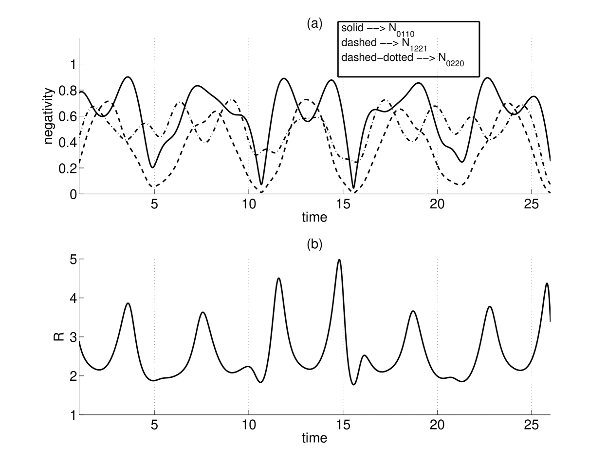
Figure 3: (a) Negativities $N_{0110}$, $N_{0220}$, and $N_{1221}$ and (b) parameter $R$ indicating violation of the Cauchy-Schwartz inequality violation as they depend of scaled time $t$. The scaled time $t$ is measured in $1/\chi_{a,b}$ units. Initial vacuum state $|0\rangle_{a}|0\rangle_{b}$ is assumed, $g=0.6$.

Figure 7: Time evolution of negativity $N_{1221}$ for $=\equiv n_{a}=n_{b}=0.1$ (solid curve), $n=0.2$ (dashed curve), and $n=0.3$ (inset); $\gamma=0.01$. The coupling $g=0.6$, other parameters and units are the same as in caption to Fig. 3.

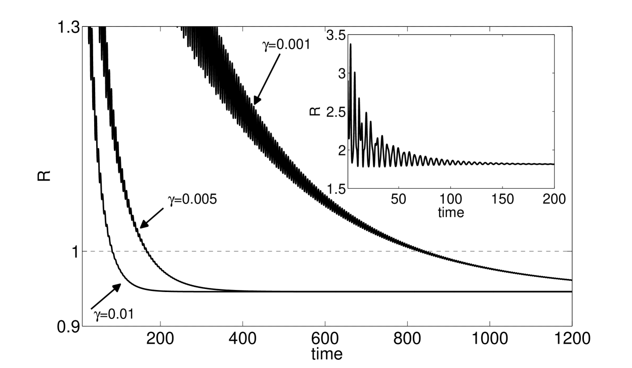
Figure 8: Temporal evolution of parameter R for damping constants $\gamma=0.001$, $0.005$, and $0.01$ assuming $\bar{n}=0.4$. For comparison, temporal evolution of parameter $R$ for zero-temperature reservoirs ($n=0$) is given for $\gamma=0.01$. The coupling $g=0.6$, Values of other parameters are the same as in caption to Fig. 3. Time $t$ is measured in $1/\chi_{a,b}$ units.

- (1) D. Loss and D.P. Di Vincenzo, Phys. Rev. A 57, 120 (1998).
- (2) J.I. Cirac and P. Zoller, Phys. Rev. Lett. 74, 4091 (1995).
- (3) J. Vidal, G. Palacios, and C. Aslangul, Phys.Rev. A 70, 062304 (2004).
- (4) Z. Ficek, Front. Phys. China, 5(1), 26 (2010).
- (5) R.W. Boyd, Nonlinear Optics (Academic Press, London, 2003), 2nd edition.
- (6) J. Peřina, Z. Hradil, and B. Jurčo Quantum Optics and Fundamentals of Physics (Kluwer Academic, Dordrecht, 1994).
- (7) D. Bouwmeester, A. Ekert, and A. Zeilinger, The Physics of Quantum Information (Springer, Berlin, 2000).
- (8) J. Řeháček, Z. Hradil, O. Haderka, J. Peřina Jr., M. Hamar, Phys Rev. A 67, 061801(R) (2003)
- (9) D. Achilles, Ch. Silberhorn, C. Sliwa, K. Banaszek, I.A. Walmsley, J. Mod. Opt. 51, 1499 (2004)
- (10) M.J. Fitch, B.C. Jacobs, T.B. Pittman, J.D. Franson, Phys. Rev. A 68, 043814 (2003)
- (11) A.J. Miller, S.W. Nam, J.M. Martinis, A.V. Sergienko, Appl. Phys. Lett. 83, 791 (2003)
- (12) O. Haderka, J. Peřina Jr., M. Hamar, J. Peřina, Phys. Rev. A 71, 033815 (2005).
- (13) M. Hamar, J. Peřina Jr., O. Haderka, V. Michálek, Phys. Rev. A 81, 043827 (2010).
- (14) J. Kim, S. Takeuchi, Y. Yamamoto, H. H. Hogue, Appl. Phys. Lett. 74, 902 (1999)
- (15) M. Bondani, A. Allevi, and A. Andreoni, Adv. Sci. Lett. 2, 463 (2009).
- (16) E. Fick and G. Sauermann, Ther Quantum Statistics of Dynamic Processes (Springer, Berlin, 1990).
- (17) D. Gottesman, Phys. Rev. A 54, 1862 (1996).
- (18) A.R. Calderbank, E.M. Rains, P.M. Shor, and N.J. Sloane, Phys. Rev. Lett. 78, 405 (1997).
- (19) P.W. Shor, Phys. Rev. A 52, 2493 (1995).
- (20) A. Ekert and C. Macchiavello, Phys. Rev. Lett. 77, 2585 (1996).
- (21) G.M. Palma, K.-A. Suominen and A.K. Ekert, Quantum Computers and Dissipation. Proc. Roy. Soc. London Ser. A, 452 (1996).
- (22) L.M Duan and G.C. Guo, Phys. Rev. A, 57, 737 (1998).
- (23) D.A. Lidar and K.B. Whaley, Irreversible Quantum Dynamics, F. Benatti and R. Floreanini (Eds.), pp. 83-120. Springer Lecture Notes in Physics vol. 622, Berlin (2003).
- (24) P.Zanardi and M Rasetti, Phys. Rev. Lett. 79, 3306 (1998).
- (25) J. Jekni -Dugić 1 and M. Dugić, Chin.Phys.Lett. 25, 371 (2008).
- (26) K. Życzkowski, P. Horodecki, M. Horodecki, and R. Horodecki, Phys.Rev. A 65, 012101 (2001).
- (27) L. Disi, Lect. Notes Phys. 622, 157 (2003).
- (28) T. Yu and J.H. Eberly, Phys. Rev. Lett. 93, 140404 (2004).
- (29) M. Ikram, F. Li, and M.S. Zubairy, Phys.Rev. A 75, 062336 (2007).
- (30) Z. Ficek and R. Tanaś, Phys.Rev. A 74, 024304 (2006).
- (31) Z. Ficek and R. Tanaś, Phys.Rev. A 74, 054301 (2008).
- (32) C.E. Lpez, G. Romero, F. Lastra, E. Solano, and J.C. Retamal, Phys.Rev.Lett. 101, 080503 (2008).
- (33) L. Mandel and E. Wolf, Optical coherence and quantum optics (Cambridge University press, Cambridge, 1995).
- (34) J. Peřina, J. Křepelka, J. Peřina Jr, M. Bondani, A. Allevi, and A. Andreoni, Eur. Phys. J. D 53, 373 (2009).
- (35) X. Li, P.L. Voss, J.E. Sharping, and P. Kumar, Phys. Rev. Lett. 94, 053601 (2005).
- (36) J. Fulconis, O. Alibart, W.J. Wadsworth, P.S. Russell, and J.G. Rarity, Opt. Express 13, 7572 (2005).
- (37) A. Sizmann and G. Leuchs, The Optical Kerr Effect and Quantum Optics in Fiber in Progress in Optics 39, ed. E.Wolf, (Elsevier Science B.V., 1999), p. 373.
- (38) X. Li, P.L. Voss, J.E. Sharping, and P. Kumar, Phys. Rev. Lett. 94, 053601 (2005).
- (39) J. Fulconis, O. Alibart, W.J. Wadsworth, P. S. Russell, and J. G. Rarity, Opt. Express 13, 7572 (2005).
- (40) A. Miranowicz and W. Leoński, J.Phys. B 39, 1683 (2006).
- (41) A. Kowalewska-Kudłaszyk and W. Leoński, Phys.Rev. A 73, 042318 (2006).
- (42) A. Kowalewska-Kudłaszyk and W. Leoński, JOSA B 73, 1289 (2009).
- (43) H. Kang and Y. Zhou, Phys. Rev. Lett. 91, 093601 (2003).
- (44) J. Bai and D.S. Citrin, Optics Express 16, 12599 (2008).
- (45) L. Spani Molella, R.-H. Rinkleff, G. Kuhn and K. Danzmann, Appl. Phys. B 90, 273 (2008).
- (46) J. Peřina, Quantum Statisics of Linear and Nonlinear Optical Phenomena (Kluwer Academic, Dordrecht, 1991) 2nd ed.
- (47) J. Peřina Jr. and J. Peřina, Quantum statistics of nonlinear optical couplers, in Progress in Optics 41, ed. E.Wolf, (Elsevier Science B.V., 2000), p. 361.
- (48) N. Korolkova and J. Peřina, Opt. Commun. 136, 135 (1996).
- (49) N. Korolkova and J. Peřina, J. Mod. Opt. 44, 1525 (1997).
- (50) J-M. Courty, S. Spälter, F. König, A. Sizmann and G. Leuchs, Phys. Rev. A 58, 1501 (1998).
- (51) L. J. Bernstein, Physica D 68 (1993) 174.
- (52) A. Chefles and S. M. Barnett J. Mod. Opt. 43 709 (1996).
- (53) M. A. Abdel-Baset, A. Ibrahim, B. A. Umarov and M. R. B. Wahiddin, Phys. Rev. A 61 (2000) 043804.
- (54) M. K. Olsen Phys. Rev. A 73 (2006) 053806.
- (55) A. Miranowicz, R. Tana s, and S. Kielich, Quant. Opt. 2, 253 (1990).
- (56) M. Kurpas, J. Dajka, and E. Zipper, J. Phys.: Condens. Matter 21, 235602 (2009).
- (57) M. Horodecki, P. Horodecki, and R. Horodecki, Phys. Lett. A 223, 1 (1996).
- (58) A. Peres, Phys. Rev. Lett. 77, 1413 (1996).
- (59) S. Hill and W.K. Wooters, Phys. Rev. Lett. 78, 5022 (1997).
- (60) J. Peřina and J. Křepelka, Optics Communications 282, 3918 (2009).
- (61) W. Li, W. Yang, X. Xie, J. Li and X. Yang, J. Phys. B 39, 3097 (2006).